1 Introduction

Even though the standard model (SM) has proved to offer a very successful description of strong and electroweak interactions, it fails in providing an explanation to issues such as the gauge group, the number of families, the dynamics of flavour and the mechanism of mass generation, among others. A particularly puzzling topic is that of the number of quark and lepton generations. From a phenomenological and experimental point of view, we have strong reasons to accept that there are indeed only three copies of up- and down-type quarks, as well of charged leptons and active neutrinos. However, on the theoretical side, there is little hint to the origin of this three-fold replication. The cancellation of anomalies requires identical number of quark and lepton families, but adds no information to the total number. Extensions of the SM, such as supersymmetry (SUSY), or grand unified theories (GUT), remedy several deficiencies of the SM, but they also fail in explaining the number of fermion families.

Given the existence of three families of quarks and leptons, and since neither theory nor experiment impose any constraints on the number of Higgs families, one could wonder whether the same family replication takes place in the Higgs sector. In addition to being very aesthetic, this scenario is not unexpected from a theoretical point of view. In some SUSY models from strings, as is the case of the compactification of the 10 dimensional $E_{8}\times E_{8}^{\prime}$ heterotic superstring to 4 dimensions, the low-energy theory thus obtained is associated with a subgroup of the gauge group $E_{6}$. Under $E_{6}$, fermions and Higgses are assigned to the same representation, and the requirement of three families of fermions imposes replication of the Higgs content [1]. In fact, many string constructions that contain three fermion families also include Higgs family replication, as is the case of $Z_{3}$ orbifold compactifications of the heterotic superstring, which also exhibit a low-energy spectrum composed of three supersymmetric Higgs families [2, 3, 4, 5, 6, 7], and that of some D-brane models [8]. Other models that include a non-minimal Higgs content have also been extensively addressed in the literature [9, 10, 11, 12, 14, 13, 15, 17, 16, 18, 19, 20, 21, 22, 23, 24, 25]. The consequences of extending the Higgs sector are abundant, and have implications which range from the theoretical to the experimental level. For instance, and if the extra Higgses are light, the addition of these states in a minimal SUSY scenario will spoil the unification of gauge couplings around 10¹⁶ GeV. Nevertheless, in models from the heterotic string, the high energy scale is different ($\approx\,g_{\text{GUT}}\,\times\,10^{17}$ GeV), and the new states can even be helpful regarding unification [5]. Since ours is a low-energy oriented analysis, we will not consider the (more speculative) high-energy implications of the extended Higgs sector. The most challenging implication of an extended Higgs sector is perhaps the potential occurrence of tree-level flavour changing neutral currents (FCNC), mediated by the exchange of neutral Higgs states. In the SM and the minimal supersymmetric standard model (MSSM), these effects are absent at the tree-level, since the coupling of the quark-quark-Higgs mass eigenstates is flavour conserving. This arises from having the Yukawa couplings proportional to the quark mass matrices, so that diagonalising the mass matrices also diagonalises the Yukawas. Since experimental data is in good agreement with the SM predictions, the potentially large contributions arising from the tree-level interactions must be suppressed in order to have a model which is experimentally viable. In general, the most stringent limit on the flavour-changing processes emerges from the small value of the $K_{L}-K_{S}$ mass difference [10, 11].

Avoiding the FCNCs induced by the tree-level exchange of neutral Higgs bosons can be achieved by several distinct approaches, each involving a different sector of the model.

(i) Discrete symmetries. Imposing a discrete symmetry on the model ensures that only one generation of Higgs couples to quark and leptons, and completely eliminates tree level FCNCs from the predictions of the model [29, 30]. Naturally, one attempts to motivate such an assumption via topological and/or geometrical arguments. For instance, in [16, 17], adding four extra Higgs doublets to the MSSM content, and assuming that the FCNCs thus induced are suppressed via some symmetry, then the extra generations (labelled “pseudo-Higgs bosons”) do not acquire vacuum expectation values (VEVs), do not mix with the two MSSM-like doublets, nor couple to fermions. Still, the lightest of the new states is stable so that it becomes a candidate for dark matter.

(ii) Suppression of Yukawa couplings. In this case, FCNCs are not eliminated, but the Yukawa interaction responsible for the tree-level flavour violation is made small enough to render the new contributions negligible. Since the most stringent bounds are usually associated with tree level contributions to the neutral kaon mass difference ($\Delta m_{K}$), the Yukawa couplings of down and strange quarks are forced to be very small. For example, in [25], a $U(2)$ flavour symmetry was considered as the candidate symmetry to suppress FCNCs. Although this second possibility is more appealing in the sense that it does not require excluding part of the Higgs content from Higgs-matter interactions, its major shortcoming lies in the fact that in general one lacks a full theory of flavour, which would predict the Yukawa couplings, as would be the case of string theory.

(iii) Decoupling of extra Higgses. If one does not wish (or is not allowed) to impose a symmetry, or if the Yukawa couplings are not free parameters of the model, a third possibility lies in making the new Higgs states heavy enough, so that the contributions they mediate are suppressed [9, 13, 10, 11, 19]. The new states are thus decoupled, and the effective low-energy theory is very similar to the usual MSSM/SM. This possibility is sometimes the only “degree of freedom” remaining, especially in highly predictive models, where the Yukawas arise from some high-energy formulation, as is the case of string models. Nevertheless, it is important to stress that the decoupling scenario is in general achieved by enforcing very large values for some of the Higgs soft-breaking masses. This may lead to a fine-tuning scenario in association with electroweak (EW) symmetry breaking. When the decoupling approach is taken together with the suppression of Yukawa couplings (ii), it is possible to obtain Higgs spectra which manage to comply with experiment without excessively heavy Higgses [10, 11, 13, 19, 20, 21, 25].

From the above discussion, it is clear that a correct evaluation of the FCNC problem associated to multi-Higgs doublet models is indeed instrumental. In what follows, we propose to analyse the most general scenario of the MSSM extended to include three families of Higgs doublets. We do not impose any symmetry on the model, allowing for the most general formulation of both the superpotential and the SUSY soft breaking Lagrangian. We provide a generic overview of the extended Higgs sector, and discuss the minimisation of the scalar potential. In this work, we also compute the most general expression for the contribution of tree-level neutral Higgs exchange to neutral meson mass difference. Contrary to previous analyses [10, 11, 13, 19], we include the contributions from all physical (rather than interaction) Higgs states, scalar and pseudoscalar. Moreover, we take into account the mixing in the Higgs sector. Finally, as an example of how to apply our general formulation, we consider an ansatz for the Yukawa couplings along the lines of previous analyses (namely the “simple Fritzsch scheme” [31, 32, 33]), and evaluate the specific contributions to the neutral mesons mass differences. Our findings turn out to be more severe than those of previous works.

The work is organised as follows. In Section 2, we analyse the extended Higgs sector, paying special attention to the minimisation of the Higgs potential and addressing potential fine-tuning issues. We compute the tree level mass matrices in Section 3 and discuss the associated spectra. Section 4 is devoted to the analysis of Higgs-matter interactions, and in Section 5 we derive a model independent computation of the tree-level contributions to the neutral meson mass differences. Assuming an illustrative example for the Yukawa couplings, we present in Section 6 a numerical study of the FCNC contributions, investigating how the Higgs spectrum must be constrained in order to have compatibility with experimental data. Finally we summarise the most relevant points in Section 7.

2 Extended Higgs sector

We begin our analysis by addressing the Higgs sector of a SUSY model where three generations of $SU(2)$ doublet superfields are comprised. In each generation, one finds hypercharge $-1/2$ and $+1/2$ fields, coupling to down- and up-quarks, respectively:

$$\widehat{H}_{1(3,5)}=\left(\begin{array}[]{c}\widehat{h}^{0}_{1(3,5)}\\ \widehat{h}^{-}_{1(3,5)}\end{array}\right)\,,\quad\quad\widehat{H}_{2(4,6)}=\left(\begin{array}[]{c}\widehat{h}^{+}_{2(4,6)}\\ \widehat{h}^{0}_{2(4,6)}\end{array}\right)\,.$$ (1)

2.1 Tree-level Higgs potential

The most general superpotential of a model with three families of Higgs doublets can be written as follows:

$$W =\,\widehat{Q}\,(Y_{1}^{d}\widehat{H}_{1}+Y_{3}^{d}\widehat{H}_{3}+Y_{5}^{d}\widehat{H}_{5})\widehat{D}^{c}+\widehat{L}\,(Y_{1}^{e}\widehat{H}_{1}+Y_{3}^{e}\widehat{H}_{3}+Y_{5}^{e}\widehat{H}_{5})\widehat{E}^{c}$$

$$+\,\widehat{Q}\,(Y_{2}^{u}\widehat{H}_{2}+Y_{4}^{u}\widehat{H}_{4}+Y_{6}^{u}\widehat{H}_{6})\widehat{U}^{c}+\mu_{12}\widehat{H}_{1}\widehat{H}_{2}+\mu_{14}\widehat{H}_{1}\widehat{H}_{4}+\mu_{16}\widehat{H}_{1}\widehat{H}_{6}$$

$$+\,\mu_{32}\widehat{H}_{3}\widehat{H}_{2}+\mu_{34}\widehat{H}_{3}\widehat{H}_{4}+\mu_{36}\widehat{H}_{3}\widehat{H}_{6}+\mu_{52}\widehat{H}_{5}\widehat{H}_{2}+\mu_{54}\widehat{H}_{5}\widehat{H}_{4}+\mu_{56}\widehat{H}_{5}\widehat{H}_{6}\,.$$ (2)

Above, $\widehat{Q}$ and $\widehat{L}$ denote the quark and lepton $SU(2)_{L}$ doublet superfields, $\widehat{U}^{c}$ and $\widehat{D}^{c}$ are quark singlets, $\widehat{E}^{c}$ the lepton singlet, and $Y_{i}^{q}$ are the Yukawa matrices associated with each Higgs superfield. Regarding the $\mu$-terms, these are now extended in order to include all possible bilinear Higgs terms. Calling upon some specific model that would be responsible for generating the latter terms, it would be possible to reduce the number of free parameters. It is also important to recall that one could also impose a (discrete) symmetry acting on the superpotential, whose effect would be the suppression of some of the couplings in $W$. However, in our discussion, we consider the most generic form for $W$, thus taking the several bilinear parameters in $W$ as effective $\mu$-terms.

From the above one can derive the $F$- and $D$-terms, writing the latter in doublet component for simplicity:

$$V_{F}\,= \operatornamewithlimits{\sum}_{\begin{smallmatrix}{i,j=1,3,5}\\ {l=2,4,6}\end{smallmatrix}}\mu^{*}_{il}\,\mu_{jl}\,H_{i}^{\dagger}\,H_{j}+\operatornamewithlimits{\sum}_{\begin{smallmatrix}{i=1,3,5}\\ {k,l=2,4,6}\end{smallmatrix}}\mu^{*}_{il}\,\mu_{ik}\,H_{k}^{\dagger}\,H_{l}\,,$$

$$V_{D}\,= \,\,\frac{g^{2}}{8}\,\operatornamewithlimits{\sum}_{a=1}^{3}\left[\operatornamewithlimits{\sum}_{i=1}^{6}H_{i}^{\dagger}\,\tau^{a}\,H_{i}\right]^{2}+\,\frac{g^{\prime 2}}{8}\left[\operatornamewithlimits{\sum}_{i=1}^{6}(-1)^{i}\left|H_{i}\right|^{2}\right]^{2}\,,$$ (3)

where $H_{i}$ are the scalar doublets belonging to the superfields of Eq. (1), $g$, $g^{\prime}$ denote the gauge coupling constants, and $\tau^{a}$ are the $SU(2)_{L}$ generators. The soft SUSY-breaking terms trivially generalise the minimal two-doublet case, including the usual soft-breaking masses and $B\mu$-like terms in the Higgs potential.

$$V_{\text{soft}}= \operatornamewithlimits{\sum}_{i,j=1,3,5}(m^{2}_{d})_{ij}\,H_{i}^{\dagger}\,H_{j}+\operatornamewithlimits{\sum}_{k,l=2,4,6}(m^{2}_{u})_{kl}\,H_{k}^{\dagger}\,H_{l}-\operatornamewithlimits{\sum}_{\begin{smallmatrix}{i=1,3,5}\\ {l=2,4,6}\end{smallmatrix}}\left[(B\mu)_{il}\,H_{i}\,H_{l}+\text{H.c.}\right]\,.$$ (4)

2.2 Minimisation of the potential: the superpotential basis and the Higgs basis

After electroweak symmetry breaking, the neutral components of the six Higgs doublets develop the following VEVs,

$$\langle h^{0}_{1(3,5)}\rangle=w_{1(3,5)}\,,\quad\quad\quad\langle h^{0}_{2(4,6)}\rangle=w_{2(4,6)}\,,$$ (5)

and as usual one can write

$$h^{0}_{i}\to w_{i}+\frac{1}{\sqrt{2}}\left(\sigma_{i}+i\varphi_{i}\right)\,.$$ (6)

In the above we assume that all the VEVs are real. The next step is to minimise the scalar potential with respect to the VEVs. Although the problem appears to be a simple generalisation of the two-Higgs doublet model (MSSM), it will prove to be much more involved. It happens that in the presence of six non-vanishing VEVs, finding a solution to the minima equations is a rather cumbersome task. As an illustration, we present the equations obtained from minimising with respect to the down-type Higgs:

$$\sum_{i=1,3,5}\left[(m^{2}_{d})_{ji}+\sum_{l=2,4,6}\mu_{jl}^{*}\,\mu_{il}\,\right]w_{i}-\sum_{l=2,4,6}(B\mu)_{jl}\,w_{l}+w_{j}\,\frac{1}{2}\,M_{Z}^{2}\,\frac{v_{d}^{2}-v_{u}^{2}}{v_{d}^{2}+v_{u}^{2}}=0\,,$$ (7)

where $j=1,3,5$ and we have defined

$$v_{d}\equiv \sqrt{w_{1}^{2}+w_{3}^{2}+w_{5}^{2}}\,,$$

$$v_{u}\equiv \sqrt{w_{2}^{2}+w_{4}^{2}+w_{6}^{2}}\,.$$ (8)

In addition to Eq. (7), which only ensure that we are in the presence of an extremum, we have to further impose the conditions for a minimum with respect to the several variables. Therefore, and for the down-type Higgs fields, having positive second derivatives is equivalent to the following inequalities:

$$(m^{2}_{d})_{jj}+\sum_{l=2,4,6}\mu_{jl}^{*}\,\mu_{jl}+\frac{1}{2}\,M_{Z}^{2}\,\left(\,\frac{v_{d}^{2}-v_{u}^{2}+2\,w_{j}^{2}}{v_{d}^{2}+v_{u}^{2}}\,\right)\,>\,0\,,$$ (9)

provided that at the minimum the determinant of the six-dimensional matrix is positive, or equivalently, $\det(\partial^{2}\,V\,/\,\partial h^{0}_{i}\,\partial h^{0}_{j})\,>0$.

The equations for the remaining cases (minimising with respect to the up-type Higgs fields) can be obtained from Eqs. (7,9) by interchanging $\{1,3,5\}\leftrightarrow\{2,4,6\}$ and changing the sign in the terms proportional to $M_{Z}^{2}$ as $M_{Z}^{2}(v_{d}^{2}-v_{u}^{2})\to-M_{Z}^{2}(v_{d}^{2}-v_{u}^{2})$ (cf. Eq. (7)) and $M_{Z}^{2}(v_{d}^{2}-v_{u}^{2}+2w^{2})\to-M_{Z}^{2}(v_{d}^{2}-v_{u}^{2}-2w^{2})$ (cf. Eq. (9)). The only choice of parameters that would render the solution of the minima equations straightforward is to call upon the diagonal soft breaking masses ($(m_{d})_{ii}$ and $(m_{u})_{kk}$) to be fixed by the minima equations. For $(m_{d})^{2}_{11}$ the minimum equation would read

$$(m_{d})^{2}_{11}= \sum_{j=2,4,6}(B\mu)_{1j}\,\frac{w_{j}}{w_{1}}-(m^{2}_{d})_{13}\,\frac{w_{3}}{w_{1}}-(m^{2}_{d})_{15}\,\frac{w_{5}}{w_{1}}$$

$$-\sum_{i=1,3,5}\,(\sum_{l=2,4,6}\mu_{1l}^{*}\mu_{il}\,\frac{w_{i}}{w_{1}}\,)-\frac{1}{2}M_{Z}^{2}\,\frac{v_{d}^{2}-v_{u}^{2}}{v_{d}^{2}+v_{u}^{2}}\,.$$ (10)

Naturally, the equations can be solved for a distinct set of parameters, but then finding an analytical solution is in general not possible. Analytical relations are very useful when writing down the mass matrices for the several Higgs sectors, since one can directly replace the parameters. In fact, the major handicap when relying on the diagonal soft masses as the minimum parameters is that then one loses control of the leading contributions to the Higgs boson mass eigenvalues. This will be made clear in a forthcoming section. Another shortcoming is that, even though we can define a generalised expression for $\tan\beta$ as $\tan\beta=\sqrt{w_{2}^{2}+w_{4}^{2}+w_{6}^{2}}\,/\,\sqrt{w_{1}^{2}+w_{3}^{2}+w_{5}^{2}}$, writing the minimisation equations as a function of $\sin\beta$, $\cos\beta$ (in an MSSM-like fashion), is impossible.

So far we have been working in the basis that naturally emerges from both the superpotential and soft-breaking Lagrangian formulation. To simplify the discussion, we will henceforth label this natural basis as the superpotential basis. However, this need not be the unique approach when addressing the minimisation of the potential.

As it has been shown, one can work in a basis where only two of the new six neutral fields have non-vanishing VEVs, the so-called Higgs basis [9, 15]. For the down-type Higgses, the new fields, $\phi_{i}$, are related to the original ones by means of the following unitary transformation, $P_{d}$:

$$\phi^{0}_{1}\equiv\frac{1}{\sqrt{w_{1}^{2}+w_{3}^{2}+w_{5}^{2}}}\,\left(w_{1}\,h^{0}_{1}+w_{3}\,h^{0}_{3}+w_{5}\,h^{0}_{5}\right)\,,$$ (11)

$$\phi^{0}_{3}\equiv\frac{1}{\sqrt{w_{1}^{2}+w_{3}^{2}+w_{5}^{2}}}\left[\sqrt{w_{3}^{2}+w_{5}^{2}}\,h^{0}_{1}-\frac{w_{1}}{\sqrt{w_{3}^{2}+w_{5}^{2}}}(w_{3}\,h^{0}_{3}+w_{5}\,h^{0}_{5})\right]\,,$$ (12)

$$\phi^{0}_{5}\equiv\frac{1}{\sqrt{w_{3}^{2}+w_{5}^{2}}}\left(w_{5}\,h^{0}_{3}-w_{3}\,h^{0}_{5}\right)\,.$$ (13)

An analogous transformation, $P_{u}$, can be derived for the up-quark-coupling Higgses ($h^{0}_{2,4,6}$), with the adequate replacements ($\{1,3,5\}\to\{2,4,6\}$). For simplicity, let us introduce the following global parametrisation for the transformations $P_{d}$ and $P_{u}$:

$$\phi_{i}=P_{ij}h_{j}\,,$$ (14)

where $P_{ij}$ is a $6\times 6$ matrix whose entries are defined from $P_{d}$ and $P_{u}$ as

$$P_{ij}=\left\{\begin{array}[]{ll}(P_{d})_{\frac{i+1}{2}\frac{j+1}{2}}&\,\,\,i,j=1,3,5\\ (P_{u})_{\frac{i}{2}\frac{j}{2}}&\,\,\,i,j=2,4,6\\ \,\,\,\,0&\,\,\,\,\,\text{elsewhere}\,.\end{array}\right.$$ (18)

From the above, it is clear that in the new basis only two of the fields do have a VEV

$$\langle\phi^{0}_{1}\rangle=\,v_{d}\,,\quad\quad\langle\phi^{0}_{2}\rangle=\,v_{u}\,,$$ (19)

with $v_{d,u}$ defined in Eq. (2.2), which in turn must satisfy

$$v_{u}^{2}+v_{d}^{2}=2\,M_{Z}^{2}/(g^{2}+g^{\prime 2})\approx(174\text{ GeV})^{2}\,,$$ (20)

where $M_{Z}$ is the mass of the $Z^{0}$ boson. In this basis one has the additional advantage that, similar to what occurs in the MSSM case, one can clearly define $\tan\beta$:

$$\tan\beta=\frac{v_{u}}{v_{d}}\,.$$ (21)

We can now write

$$\phi^{0}_{1,2}\to v_{d,u}+\frac{1}{\sqrt{2}}\left(R_{1,2}+iI_{1,2}\right)\,,$$

$$\phi^{0}_{i}\to\frac{1}{\sqrt{2}}\left(R_{i}+iI_{i}\right)\,\quad\quad i=3-6\,.$$ (22)

Thus, one can now understand the three Higgs family model as an MSSM-like model, extended by 4 additional doublets, which do not directly interfere with the mechanism of electroweak symmetry breaking. In the Higgs basis, the potential preserves its original structure with respect to the dependence on the field combination, but the parameters associated with the $F$- and soft breaking terms are now redefined as

$$V_{F}\,= \operatornamewithlimits{\sum}_{\begin{smallmatrix}{a,b=1,3,5}\\ {l=2,4,6}\end{smallmatrix}}\bar{\mu}^{l}_{ab}\,\phi_{a}^{\dagger}\,\phi_{b}+\operatornamewithlimits{\sum}_{\begin{smallmatrix}{i=1,3,5}\\ {c,d=2,4,6}\end{smallmatrix}}\bar{\bar{\mu}}^{i}_{cd}\,\phi_{c}^{\dagger}\,\phi_{d}\,,$$

$$V_{\text{soft}}\,= \operatornamewithlimits{\sum}_{a,b=1,3,5}(\bar{m}^{2}_{d})_{ab}\,\phi_{a}^{\dagger}\,\phi_{b}+\operatornamewithlimits{\sum}_{c,d=2,4,6}({\bar{\bar{m}}}^{2}_{u})_{cd}\,\phi_{c}^{\dagger}\,\phi_{d}-\operatornamewithlimits{\sum}_{\begin{smallmatrix}{a=1,3,5}\\ {c=2,4,6}\end{smallmatrix}}\left[(\overline{B\mu})_{ac}\,\phi_{a}\,\phi_{c}+\text{H.c.}\right]\,,$$ (23)

where

$$\bar{\mu}^{l}_{ab}=(P_{d})_{ai}\,\mu^{*}_{il}\,\mu_{jl}\,(P_{d}^{\dagger})_{jb}\,,\quad\quad\quad\quad\quad\bar{\bar{\mu}}^{i}_{cd}=(P_{u})_{cl}\,\mu^{*}_{il}\,\mu_{ik}\,(P_{u}^{\dagger})_{kd}\,,$$

$$(\bar{m}^{2}_{d})_{ab}=(P_{d})_{ai}\,(m^{2}_{d})_{ij}\,(P_{d}^{\dagger})_{jb}\,,\quad\quad\quad({\bar{\bar{m}}}^{2}_{u})_{cd}=(P_{u})_{ck}\,(m^{2}_{u})_{kl}\,(P_{u}^{\dagger})_{ld}\,,$$

$$(\overline{B\mu})_{ac}=(P_{d}^{\dagger})_{ia}\,(B\mu)_{il}\,(P_{u}^{\dagger})_{lc}\,,\quad\quad\quad i,j,a,b=1,3,5\,;\quad\quad k,l,c,d=2,4,6\,.$$ (24)

In the new basis, the problem of minimising the scalar potential is quite simplified, and one is able to derive the six minimisation conditions in a compact form. The conditions for the down-type sector read

$$m^{2}_{11}\,= \,\,b_{12}\,\tan\beta-\frac{M_{Z}^{2}}{2}\,\cos 2\beta\,,$$

$$m^{2}_{13}\,= \,\,b_{32}\,\tan\beta\,,$$

$$m^{2}_{15}\,= \,\,b_{52}\,\tan\beta\,,$$ (25)

while those related to the up-type Higgses are given by

$$m^{2}_{22}\,= \,\,b_{12}\,\cot\beta+\frac{M_{Z}^{2}}{2}\,\cos 2\beta\,,$$

$$m^{2}_{24}\,= \,\,b_{14}\,\cot\beta\,,$$

$$m^{2}_{26}\,= \,\,b_{16}\,\cot\beta\,.$$ (26)

In the above, and for simplicity, we have introduced the short-hand notation

$$m_{ij}^{2} =\left\{\begin{array}[]{l}\operatornamewithlimits{\sum}_{l=2,4,6}\,\bar{\mu}^{l}_{ij}+(\bar{m}_{d}^{2})_{ij}\quad\quad i,j=1,3,5\\ \operatornamewithlimits{\sum}_{k=1,3,5}\,\bar{\bar{\mu}}^{k}_{ij}+(\bar{\bar{m}}_{u}^{2})_{ij}\quad\quad i,j=2,4,6\,,\end{array}\right.$$ (28)

$$b_{ij} =(\overline{B\mu})_{ij}\,,$$ (29)

where we stress that both parameters $\bar{\mu}_{ij}$, and $\bar{\bar{\mu}}_{ij}$, as well as $b_{ij}$ have dimensions (mass²). Throughout the paper we will be often using the above short-hand notation, even though this implies that the rotated $\mu$-terms and Higgs soft breaking masses loose their individual character, becoming merged into the quantities $m^{2}_{ij}$. As a final comment, let us notice that the minima equations (2.2,2.2) are, in structure, very similar to those of the MSSM, namely the first in each set of three. It is worth referring that the EW scale is only explicitly present in two equations (those derived with respect to $\phi^{0}_{1,2}$, the VEV-acquiring fields). Notice however, that this is a mere consequence of working in a different basis.

In addition to the minima conditions Eqs. (2.2,2.2), one can also derive other conditions, which are useful in constraining the allowed parameter space. As an example, and from direct comparison of the minima equations for $m^{2}_{11}$ and $m^{2}_{22}$, we find the following inequality:

$$m^{2}_{11}\,m^{2}_{22}\,\leq\,b^{2}_{12}\,,$$ (30)

strongly resembling the analogous MSSM condition.

2.3 Numerical minimisation of the potential: illustrative examples

In what follows, our goal is to conduct a short analysis of the issues discussed in the previous subsections. The phenomenological analysis of the Higgs sector (masses and mixings) will be carried in detail in Section 3, working in the Higgs basis. Nevertheless, we find it interesting to evaluate how the minimisation of the scalar potential constrains the soft breaking terms. To do so, we consider several numerical examples for the minimisation of the scalar potential for distinct VEV regimes. In addition, we also discuss whether or not a specific choice of soft breaking terms may translate into a fine-tuning problem. Although the minima conditions are cast in a much more compact and appealing way in the Higgs basis, since only two of them explicitly involve the EW scale, a possible fine tuning problem may be unapparent in this case. Therefore, for this specific discussion, we will stick to the original superpotential basis. In this case, and since we make no assumptions regarding the mechanism of SUSY breaking associated with this generic multi-Higgs doublet model, we take the input parameters

$$(m_{d}^{2})_{ij}\,,\ \ (m_{u}^{2})_{ij}\,,\ \ \mu_{ij}\,,\ \ (B\mu)_{ij}\,,$$ (31)

to be free at the electroweak scale. Regarding the Higgs VEVs ($w_{i}$), we impose no constraint other than satisfying the EW breaking conditions for a given value of $\tan\beta$. In order to further simplify the approach, we will fix, in each separate analysis, the value of $\mu_{ij}=\mu$, and assume a common overall scale for the off-diagonal masses $(m_{d})_{ij}$ and $(m_{u})_{ij}$, and for $(B\mu)_{ij}$. More specifically, we take universal $B\mu$ terms, $(B\mu)_{ij}=B\mu=M_{S}^{2}$, where $M_{S}$ is a “typical soft-SUSY breaking scale”. For the off-diagonal masses $(m_{d})_{ij}$ and $(m_{u})_{ij}$, the common scale is taken to be $(m_{d})_{ij}=(m_{u})_{ij}=0.1\,M_{S}$.

As discussed in the previous subsection, the parameters which are (trivially) fixed by the six minima equations are the diagonal Higgs soft-breaking masses, $(m_{d}^{2})_{ii}$ and $(m_{u}^{2})_{ii}$. Clearly, from Eq. (2.2), the minima values for $(m^{2}_{q})_{ii}$, and in particular those of the down-type Higgs sector, will be very dependent of the values of the VEVs considered, most specifically on whether one chooses a degenerate or hierarchical regime. Therefore, each case has to be separately investigated, and in each situation, one must analyse the impact of the other free parameters, namely that of the overall scale chosen for the soft-breaking parameters.

In addition, one has to investigate whether or not the parameters taken lead to a potential fine tuning (FT) problem for the parameters. In doing so, our approach will be the following. For a specific scenario defined by the parameters in Eq. (31), together with $w_{i}$ and $\tan\beta$, we compute the values of the diagonal soft breaking masses, as imposed from complying with the minima equations. We then impose a tiny perturbation on the solutions,

$$(m^{2}_{q})_{ii}\,\to\,(m^{2}_{q})_{ii}^{\prime}\,=\,(1+\lambda^{q})\,(m^{2}_{q})_{ii}\,,$$ (32)

where $\lambda$ is taken to be around a few percent. Finally, we compute the new value of $M_{Z}$ derived from perturbing the correct (true minima) solution for $(m^{2}_{q})_{ii}$, $M_{Z}^{\prime}$. To evaluate the amount of FT, we follow [35, 36], and introduce the parameter $\Delta p$, defined as

$$\Delta p_{i}\,\frac{\delta p_{i}}{p_{i}}\,=\,\frac{\delta M_{Z}^{2}}{M_{Z}^{2}}\,,$$ (33)

identifying $p_{i}$ with $(m^{2}_{q})_{ii}$. A rough measure of the fine-tuning can be derived from $(\Delta p_{i})^{-1}$, since the latter can be identified with the probability of a cancellation between terms of a given size to obtain a final result $\Delta p_{i}$ times smaller.

In what follows we take, as illustrative examples, two distinct cases for the Higgs VEVs: degenerate and hierarchical $w_{i}$. We stress here that at this point we are only investigating the constraints on the soft breaking terms arising from the minima conditions. A study of the spectrum is far simplified when moving to Higgs basis, as will be done in the following Section.

$\bullet$ Degenerate VEVs: $w_{1}=w_{3}=w_{5}$, $w_{2}=w_{4}=w_{6}$

In this case, the minima equations become much simpler, since in each sector the VEVs factor out. Therefore, having fixed the free parameters as above described, the six original equations essentially reduce to two independent ones: one for the down-type Higgs (e.g. $(m_{d})^{2}_{11}$) and another for the up-type sector (e.g. $(m_{u})^{2}_{22}$).

In Fig. 1, we plot $(m_{d})^{2}_{11}$ and $(m_{u})^{2}_{22}$, as computed from the tree-level minima equations, as a function of the common soft breaking term scale, $M_{S}$, for $\mu_{ij}=\mu=200$ GeV. In each case, we consider two distinct values for $\tan\beta$: 5 and 10.

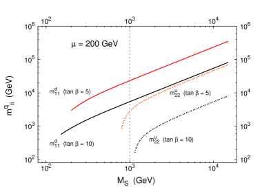
Figure 1: Minima solutions $m^{d}_{11}$ and $m^{u}_{22}$ as a function of the common SUSY breaking scale $M_{S}$ for $\tan\beta=$5, 10 and degenerate VEVs. To the left of the vertical dotted line, the solutions for $m^{q}_{ii}$ are not true minima of the potential.

From Fig. 1, several properties of this model become apparent. First of all, it becomes clear that in this basis (the superpotential basis) finding minima can be a challenging task. Notice that although one can find solutions for the down-type sector associated with low $M_{S}$, in this range we are in the presence of maxima (rather than minima) for the up-type soft masses. The situation slightly worsens with increasing $\tan\beta$. Taking other (higher) values of $\mu$ would lead to the displacement of the vertical line further to the right of the parameter space parametrised by $M_{S}$. This behaviour can be confirmed by inspection of Eqs. (7,9,2.2).

Let us now evaluate how fine-tuned these solutions are. In Fig. 2 we investigate $\Delta p$ for the up and down sectors, by studying in each case the effect of perturbing the minima solutions $(m^{d}_{11})^{2}$ and $(m^{u}_{22})^{2}$ by $\lambda^{d,u}=1\%$ and $\lambda^{d,u}=5\%$. We again consider $\mu=200$ GeV, and take $\tan\beta=10$.

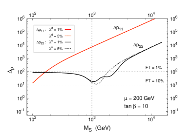
Figure 2: $\Delta p$ as a function of the SUSY scale $M_{S}$ for perturbations of 1% and 5% in $(m^{d}_{11})^{2}$ and $(m^{u}_{22})^{2}$. $\mu=200$ GeV, and $\tan\beta=10$ (the two lines for $\Delta p_{11}$ appear over-set). To the left of the vertical dotted line, the solutions for $m^{q}_{ii}$ are not true minima of the potential. Horizontal lines denote areas above which one roughly expects a FT stronger than 1% and 10%.

From Eqs. (32,33) together with the minimisation conditions in Eq. (2.2), it is apparent that $\Delta p_{i}\propto\frac{(m_{q}^{2})_{ii}}{M_{Z}^{2}}$. Moreover, it can be clearly seen that for the down-type sector, the dominant term ($B\mu$) is further enhanced by a factor of $\tan\beta$, so that a tiny fluctuation in $(m^{d}_{11})^{2}$ is not easily cancelled. In the up-type masses, the situation is reversed. The up-type version of Eq. (2.2) would exhibit a suppression of $B\mu$ by $\cot\beta$, so that here we find a more relaxed scenario.

$\bullet$ Hierarchical VEVs: $w_{5}=10\,w_{3}=100\,w_{1}$, $w_{6}=10\,w_{4}=100\,w_{2}$

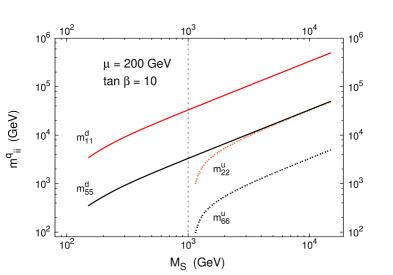
Figure 3: Minima solutions for non-degenerate VEVs as a function of the SUSY scale $M_{S}$, with $\mu=200$ GeV, and $\tan\beta=$10. To the left of the vertical dotted line, the solutions for $m^{q}_{ii}$ are not true minima of the potential.

In this case, and when compared to the degenerate one, each soft mass exhibits a very distinct behaviour at the minima of the potential. We will thus analyse the solutions which in each case are associated with the lightest and heaviest VEV, $(m_{d})^{2}_{11}$, $(m_{u})^{2}_{22}$ and $(m_{d})^{2}_{55}$, $(m_{u})^{2}_{66}$. As before, in Fig. 3 we display the above masses as a function of $M_{S}$ for $\mu=200$ GeV, and $\tan\beta=$10, similar to what was presented for degenerate VEVs in Fig. 1. As seen from Fig. 3, the range for the solutions is not strongly affected. Notice however that the minima values of $(m_{u})^{2}_{22}$ and $(m_{d})^{2}_{55}$ become degenerate for large values of $M_{S}$. Moreover, the soft mass associated with the largest VEV ($m^{u}_{66}$) presents, as expected, much smaller values than the others. This is a consequence of the suppression of $w_{j}/w_{6}$ on $B\mu$. Regarding the fine tuning, the situation is more involved. In Fig. 4 we plot $\Delta p$ for the up and down sectors, considering only the effect of a $\lambda^{d,u}=\lambda=1\%$ perturbation in $(m^{u}_{22})^{2}$, $(m^{u}_{44})^{2}$, $(m^{d}_{55})^{2}$ and $(m^{u}_{66})^{2}$. We take $\mu=200$ GeV and $\tan\beta=10$.

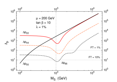
Figure 4: $\Delta p$ as a function of the SUSY scale $M_{S}$ for perturbations of 1% in the diagonal soft masses, for non-degenerate VEVS. We take $\mu=$200 GeV and $\tan\beta=$10. To the left of the vertical dotted line, the solutions for $m^{q}_{ii}$ are not true minima of the potential. Horizontal lines denote areas above which one roughly expects a FT stronger than 1% and 10%.

As seen from Fig. 4, the alterations emerge in both up- and down-type Higgs sectors. Regarding the down-type scalar ($\Delta p_{55}$) the fine tuning is typically larger now, and the effect is essentially due to the fact that it is now much more difficult to find cancellations among the several terms entering in the minimisation equations. In the up-type sector, we find a very similar situation to that of Fig. 2 for the second and third generations (associated with the larger VEVs). Conversely, and since it is now associated to a tiny VEV, the first generation up-type diagonal soft mass is more unstable under perturbations, and its behaviour merges with that of $(m^{d}_{55})^{2}$ for larger values of $M_{S}$.

It has been shown in the MSSM that with a soft SUSY scale of a few hundred GeV the associated FT is around the level of 10% [36]. When compared to the MSSM, this extended model offers a more problematic FT scenario, as is manifest in Figs. 2 and 4. This can also be seen from the comparison of Eq. (2.2) with its MSSM counterpart. In addition to the single $(B\mu)_{12}$ and $\mu^{2}_{12}$ terms, one now encounters additional $(B\mu)_{1j}$ and $\mu_{1l}\mu_{il}$, as well as new soft breaking masses on the right hand-side of the above equation, which must cancel out to achieve the correct value of $M_{Z}$.

Finally, and even though in our analysis the VEVs were not fit by the minima equations, but taken as input parameters instead, let us consider the effect of imposing a small perturbation on the VEVs, while keeping the other parameters as defined either by input values and/or minima conditions. As for the previous case of perturbing the minima values of $m^{q}_{ii}$, we now impose that

$$w_{i}\,\to\,w_{i}^{\prime}\,=\,(1+\rho^{q})\,w_{i}\,.$$ (34)

In Fig. 5, we plot the effect on $M_{Z}$ (parametrised by $\Delta p$) arising from taking $\rho^{d}=\rho^{u}=\rho=1\,\%$ for the case of degenerate (left) and non-degenerate VEVs (right). Again we consider $\mu=$ 200 GeV and $\tan\beta=10$.igs/

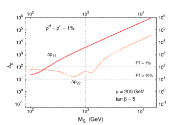
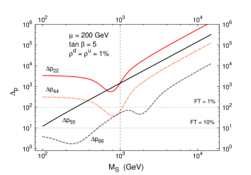
Figure 5: $\Delta p$ as a function of the common SUSY scale $M_{S}$ for perturbations of 1% in $w_{i}$, for $\mu=$200 GeV and $\tan\beta=10$. On the left we present the degenerate VEV case, on the right the non-degenerate case.

It suffices to comment that the larger the VEVs, the more stable they are under perturbations, and this effect is particularly manifest for the non-degenerate VEV case.

3 Tree-level Higgs mass matrices

We are now in conditions to investigate the Higgs spectrum, which will contain eleven neutral states, and ten charged physical particles. Let us begin with the derivation of the tree level mass matrices for the charged scalars.

3.1 Charged Higgses

In the basis defined by ($\phi^{-}_{1},\phi^{+*}_{2},\phi_{3}^{-},\phi_{4}^{+*},\phi_{5}^{-},\phi_{6}^{+*}$), the scalar potential for the charged components reads,

$$V^{\pm}= \sum_{i=1,3,5}m_{i}^{2}\,|\phi_{i}^{-}|^{2}+\sum_{i=2,4,6}m_{i}^{2}\,|\phi_{i}^{+}|^{2}+\frac{g^{2}+g^{\prime 2}}{8}\,\sum_{i=1}^{6}\,|H_{i}|^{2}\,|H_{i}|^{2}+\frac{g^{2}}{4}\,\sum_{\begin{subarray}{c}i,j=1\\ i\neq j\end{subarray}}^{6}|H_{i}^{\dagger}\,H_{j}|^{2}$$

$$-\frac{g^{2}+g^{\prime 2}}{8}\sum_{\begin{subarray}{c}i,j=1\\ i+j=\text{odd}\end{subarray}}^{6}|H_{i}|^{2}\,|H_{j}|^{2}-\,\frac{g^{2}-g^{\prime 2}}{8}\sum_{\begin{subarray}{c}i,j=1\\ i+j=\text{even}\\ i\neq j\end{subarray}}^{6}|H_{i}|^{2}\,|H_{j}|^{2}+(m_{13}^{2}\,\phi_{1}^{-*}\,\phi_{3}^{-}$$

$$+m_{15}^{2}\,\phi_{1}^{-*}\,\phi_{5}^{-}+m_{35}^{2}\,\phi_{3}^{-*}\,\phi_{5}^{-}+m_{24}^{2}\,\phi_{2}^{+*}\,\phi_{4}^{+}+m_{26}^{2}\,\phi_{2}^{+*}\,\phi_{6}^{+}+m_{46}^{2}\,\phi_{4}^{+*}\,\phi_{6}^{+}$$

$$+\mathrm{H.c.})+(b_{12}\,\phi_{1}^{-}\,\phi_{2}^{+}+b_{14}\,\phi_{1}^{-}\,\phi_{4}^{+}+b_{16}\,\phi_{1}^{-}\,\phi_{6}^{+}+b_{32}\,\phi_{3}^{-}\,\phi_{2}^{+}+b_{34}\,\phi_{3}^{-}\,\phi_{4}^{+}$$

$$+b_{36}\,\phi_{3}^{-}\,\phi_{6}^{+}+b_{52}\,\phi_{5}^{-}\,\phi_{2}^{+}+b_{54}\,\phi_{5}^{-}\,\phi_{4}^{+}+b_{56}\,\phi_{5}^{-}\,\phi_{6}^{+}+\mathrm{H.c.})\,.$$ (35)

At the minimum of the potential, the mass matrix for the charged states is:

$$\mathcal{M}_{\pm}^{2}=\left(\begin{array}[]{cccccc}\scriptscriptstyle{b_{12}\tan\beta+M_{W}^{2}\sin^{2}\beta}&\scriptscriptstyle{b_{12}+\frac{1}{2}M_{W}^{2}\sin 2\beta}&\scriptscriptstyle{b_{32}\tan\beta}&\scriptscriptstyle{b_{14}}&\scriptscriptstyle{b_{52}\tan\beta}&\scriptscriptstyle{b_{16}}\\ \scriptscriptstyle{b_{12}+\frac{1}{2}M_{W}^{2}\sin 2\beta}&\scriptscriptstyle{b_{12}\cot\beta}+M_{W}^{2}\cos^{2}\beta&\scriptscriptstyle{b_{32}}&\scriptscriptstyle{b_{14}\cot\beta}&\scriptscriptstyle{b_{52}}&\scriptscriptstyle{b_{16}\cot\beta}\\ \scriptscriptstyle{b_{32}\tan\beta}&\scriptscriptstyle{b_{32}}&\scriptscriptstyle{m_{33}^{2}-T_{W}}&\scriptscriptstyle{b_{34}}&\scriptscriptstyle{m_{35}^{2}}&\scriptscriptstyle{b_{36}}\\ \scriptscriptstyle{b_{14}}&\scriptscriptstyle{b_{14}\cot\beta}&\scriptscriptstyle{b_{34}}&\scriptscriptstyle{m_{44}^{2}+T_{W}}&\scriptscriptstyle{b_{54}}&\scriptscriptstyle{m_{46}^{2}}\\ \scriptscriptstyle{b_{52}\tan\beta}&\scriptscriptstyle{b_{52}}&\scriptscriptstyle{m_{35}^{2}}&\scriptscriptstyle{b_{54}}&\scriptscriptstyle{m_{55}^{2}-T_{W}}&\scriptscriptstyle{b_{56}}\\ \scriptscriptstyle{b_{16}}&\scriptscriptstyle{b_{16}\cot{\beta}}&\scriptscriptstyle{b_{36}}&\scriptscriptstyle{m_{46}^{2}}&\scriptscriptstyle{b_{56}}&\scriptscriptstyle{m_{66}^{2}+T_{W}}\end{array}\right)\,,$$ (36)

where $M_{W}$ is the mass of the $W^{\pm}$ boson and $T_{W}=\frac{1}{2}M_{W}^{2}\cos(2\beta)(1-\tan^{2}\theta_{W})$. One can easily identify the massless combinations that will give rise to the charged Goldstone bosons ($G^{\pm}$), “eaten away” as the $W^{\pm}$ acquire mass. The eigenstates will be henceforth denoted by $h_{i}^{\pm}$, with $i=1$ corresponding to the unphysical massless state. The upper-left $4\times 4$ sub-matrix of the one above displayed is similar in structure to that derived in [15], in the framework of a four-Higgs doublet model.

We stress here that the compact appearance of the matrix in Eq. (36) is a direct consequence of working in the Higgs basis. From direct inspection of the above matrix, one can impose that the diagonal blocks have semi-positive eigenvalues, thus deriving a zeroth order condition for avoiding tachyonic charged states. For example, for the $(\phi_{3}^{-}-\phi_{4}^{+})$ sector, this would read:

$$m^{2}_{33}\,m^{2}_{44}\gtrsim b^{2}_{34}\,,$$ (37)

while an identical argumentation within a sector (e.g.$(\phi_{3}^{-}-\phi_{5}^{-})$ in the down-type Higgs) would in turn lead to

$$m^{2}_{33}\,m^{2}_{55}\gtrsim m^{4}_{35}\,.$$ (38)

Albeit very useful, the above equations are only necessary (rather than sufficient) conditions to ensure the presence of true minima, so they should be interpreted as a means of orientation in the parameter space. Additionally, we notice that simple conditions as those above are only possible to derive in the Higgs basis.

3.2 Neutral Higgses

In our work, we are particularly interested in the neutral Higgs bosons. In order to find the neutral spectrum of the model, we decompose the complex fields as in Eq. (2.2), and derive the mass matrices associated with the real and imaginary components. CP conservation in the Higgs sector translates in the absence of terms mixing the $R_{i}$ and $I_{i}$ components, so that scalar and pseudoscalar states do not mix. For the scalar mass matrix we obtain

$$\mathcal{M}_{R}^{2}=\frac{1}{2}\frac{\partial^{2}V}{\partial R_{i}\partial R_{j}}\Bigg{|}_{\text{min}}$$

$$\scriptstyle{=}\left(\begin{array}[]{cccccc}\scriptscriptstyle{b_{12}\tan\beta+M_{Z}^{2}\cos^{2}\beta}&\scriptscriptstyle{-b_{12}-\frac{M_{Z}^{2}}{2}\sin 2\beta}&\scriptscriptstyle{b_{32}\tan\beta}&\scriptscriptstyle{-b_{14}}&\scriptscriptstyle{b_{52}\tan\beta}&\scriptscriptstyle{-b_{16}}\\ \scriptscriptstyle{-b_{12}-\frac{M_{Z}^{2}}{2}\sin 2\beta}&\scriptscriptstyle{b_{12}\cot\beta+M_{Z}^{2}\sin^{2}\beta}&\scriptscriptstyle{-b_{32}}&\scriptscriptstyle{b_{14}\cot\beta}&\scriptscriptstyle{-b_{52}}&\scriptscriptstyle{b_{16}\cot\beta}\\ \scriptscriptstyle{b_{32}\tan\beta}&\scriptscriptstyle{-b_{32}}&\scriptscriptstyle{m_{33}^{2}+\frac{M_{Z}^{2}}{2}\cos 2\beta}&\scriptscriptstyle{-b_{34}}&\scriptscriptstyle{m_{35}^{2}}&\scriptscriptstyle{-b_{36}}\\ \scriptscriptstyle{-b_{14}}&\scriptscriptstyle{b_{14}\cot\beta}&\scriptscriptstyle{-b_{34}}&\scriptscriptstyle{m_{44}^{2}-\frac{M_{Z}^{2}}{2}\cos 2\beta}&\scriptscriptstyle{-b_{54}}&\scriptscriptstyle{m_{46}^{2}}\\ \scriptscriptstyle{b_{52}\tan\beta}&\scriptscriptstyle{-b_{52}}&\scriptscriptstyle{m_{35}^{2}}&\scriptscriptstyle{-b_{54}}&\scriptscriptstyle{m_{55}^{2}+\frac{M_{Z}^{2}}{2}\cos 2\beta}&\scriptscriptstyle{-b_{56}}\\ \scriptscriptstyle{-b_{16}}&\scriptscriptstyle{b_{16}\cot{\beta}}&\scriptscriptstyle{-b_{36}}&\scriptscriptstyle{m_{46}^{2}}&\scriptscriptstyle{-b_{56}}&\scriptscriptstyle{m_{66}^{2}-\frac{M_{Z}^{2}}{2}\cos 2\beta}\end{array}\right)\,.$$

(39)

It is straightforward to recognise the MSSM scalar Higgs mass matrix as the $2\times 2$ upper left block of the previous $6\times 6$ matrix. Likewise, the tree-level mass matrix for the pseudoscalar can be written as

$$\mathcal{M}_{I}^{2}=\frac{1}{2}\frac{\partial^{2}V}{\partial I_{i}\partial I_{j}}\Bigg{|}_{\text{min}}$$

$$=\left(\begin{array}[]{cccccc}\scriptscriptstyle{b_{12}\tan\beta}&\scriptscriptstyle{b_{12}}&\scriptscriptstyle{b_{32}\tan\beta}&\scriptscriptstyle{b_{14}}&\scriptscriptstyle{b_{52}\tan\beta}&\scriptscriptstyle{b_{16}}\\ \scriptscriptstyle{b_{12}}&\scriptscriptstyle{b_{12}\cot\beta}&\scriptscriptstyle{b_{32}}&\scriptscriptstyle{b_{14}\cot\beta}&\scriptscriptstyle{b_{52}}&\scriptscriptstyle{b_{16}\cot\beta}\\ \scriptscriptstyle{b_{32}\tan\beta}&\scriptscriptstyle{b_{32}}&\scriptscriptstyle{m_{33}^{2}+\frac{M_{Z}^{2}}{2}\cos 2\beta}&\scriptscriptstyle{b_{34}}&\scriptscriptstyle{m_{35}^{2}}&\scriptscriptstyle{b_{36}}\\ \scriptscriptstyle{b_{14}}&\scriptscriptstyle{b_{14}\cot\beta}&\scriptscriptstyle{b_{34}}&\scriptscriptstyle{m_{44}^{2}-\frac{M_{Z}^{2}}{2}\cos 2\beta}&\scriptscriptstyle{b_{54}}&\scriptscriptstyle{m_{46}^{2}}\\ \scriptscriptstyle{b_{52}\tan\beta}&\scriptscriptstyle{b_{52}}&\scriptscriptstyle{m_{35}^{2}}&\scriptscriptstyle{b_{54}}&\scriptscriptstyle{m_{55}^{2}+\frac{M_{Z}^{2}}{2}\cos 2\beta}&\scriptscriptstyle{b_{56}}\\ \scriptscriptstyle{b_{16}}&\scriptscriptstyle{b_{16}\cot{\beta}}&\scriptscriptstyle{b_{36}}&\scriptscriptstyle{m_{46}^{2}}&\scriptscriptstyle{b_{56}}&\scriptscriptstyle{m_{66}^{2}-\frac{M_{Z}^{2}}{2}\cos 2\beta}\end{array}\right)\,.$$

(40)

In the $2\times 2$ submatrix defined by the $i,j=1,2$ entries, it is easy to identify the combination associated with the massless Goldstone boson. As in the MSSM, the latter degree of freedom is “eaten” by the $Z^{0}$ boson, as it acquires a mass. After rotating away the massless state,

$$G^{0}=\frac{1}{\sqrt{2}}(I_{2}\sin\beta-I_{1}\cos\beta)\,,$$ (41)

by means of the unitary transformation

$$\left(\begin{array}[]{c}I_{1}^{\prime}\\ I_{2}^{\prime}\end{array}\right)=\left(\begin{array}[]{cc}\cos{\beta}&-\sin{\beta}\\ \sin{\beta}&\cos{\beta}\end{array}\right)\left(\begin{array}[]{c}I_{1}\\ I_{2}\end{array}\right)\,,$$ (42)

the five remaining eigenstates are in general massive, and the new mass matrix reads

$$\mathcal{M}_{I}^{{}^{\prime}2}=\left(\begin{array}[]{ccccc}\scriptstyle{\frac{2b_{12}}{\sin 2\beta}}&\scriptstyle{b_{32}\sec{\beta}}&\scriptstyle{b_{14}\csc\beta}&\scriptstyle{b_{52}\sec\beta}&\scriptstyle{b_{16}\csc\beta}\\ \scriptstyle{b_{32}\sec\beta}&\scriptstyle{m_{33}^{2}+\frac{m_{Z}^{2}}{2}\cos 2\beta}&\scriptstyle{b_{34}}&\scriptstyle{m_{35}^{2}}&\scriptstyle{b_{36}}\\ \scriptstyle{b_{14}\csc\beta}&\scriptstyle{b_{34}}&\scriptstyle{m_{44}^{2}-\frac{m_{Z}^{2}}{2}\cos 2\beta}&\scriptstyle{b_{54}}&\scriptstyle{m_{46}^{2}}\\ \scriptstyle{b_{52}\sec\beta}&\scriptstyle{m_{35}^{2}}&\scriptstyle{b_{54}}&\scriptstyle{m_{55}^{2}+\frac{m_{Z}^{2}}{2}\cos 2\beta}&\scriptscriptstyle{b_{56}}\\ \scriptstyle{b_{16}\csc\beta}&\scriptstyle{b_{36}}&\scriptstyle{m_{46}^{2}}&\scriptstyle{b_{56}}&\scriptstyle{m_{66}^{2}-\frac{m_{Z}^{2}}{2}\cos 2\beta}\end{array}\right)\,.$$ (43)

When discussing the issue of minimising the scalar potential, we pointed out that each of the presented basis (Higgs and superpotential basis) had its own advantages/drawbacks. Here we are facing a very strong point in favour of the Higgs basis, namely the possibility of rotating away the pseudoscalar massless state via a transformation that only involves the first two states. Should we have been working in the superpotential basis, the transformation of Eq. (42) would be far more complex. Even though one could still define $\tan\beta$ as $\tan\beta=\sqrt{w_{2}^{2}+w_{4}^{2}+w_{6}^{2}}\,/\,\sqrt{w_{1}^{2}+w_{3}^{2}+w_{5}^{2}}$, the rotation parametrised by $\beta$ would be extended to a $6\times 6$ matrix, which would act upon the combination of $P^{\dagger}\,(I_{1},I_{2},\dots I_{6})^{T}$.

It is worth recalling that the above mass matrices (scalar and pseudoscalar) are not those associated with the original (interaction) eigenstates. The relation between the superpotential basis and the Higgs basis is trivially obtained from Eq. (14),

$$R_{i}=P_{ij}\sigma_{j}\,,\quad\quad I_{i}=P_{ij}\varphi_{j}\,,\quad\quad i,j=1\ldots 6\,.$$ (44)

In the Higgs basis, the mass matrices can be easily diagonalised by

$$S_{R}\mathcal{M}^{2}_{R}S_{R}^{\dagger} =\Delta_{R}^{2}=\operatorname{diag}({m^{s}_{i}}^{2})\,,$$

$$S_{I}\mathcal{M}^{2}_{I}S_{I}^{\dagger} =\Delta_{I}^{2}=\operatorname{diag}({m^{p}_{i}}^{2})\,,$$ (45)

where $\Delta_{R,I}^{2}$ are the diagonal scalar and pseudoscalar squared mass eigenvalues (notice that the $i=1$ term for the pseudoscalars corresponds to the unphysical massless would-be Goldstone boson). From the above it is straightforward to observe that the matrices that diagonalise the mass matrices in the original basis can be related to the latter as

$$S_{\sigma,\varphi}\,=\,S_{R,I}\,P\,.$$ (46)

3.3 Tree-level Higgs spectrum - a brief discussion

Although a thorough analysis of the Higgs parameter space lies beyond the scope of this paper, it is important to comment on a few issues. The first regards radiative corrections, which play a key role in the MSSM and its extensions, especially in relation with the mass of the lightest scalar Higgs. Without radiative corrections, and as occurs in the MSSM, the mass of the lightest scalar is bounded to be $m_{h^{0}_{1}}\lesssim M_{Z}$ [12]. In the framework of supersymmetric models with extended Higgs sectors, higher order contributions to the lightest Higgs mass have been already analysed [37], and the upper bound on $m_{h^{0}_{1}}$ does not differ significantly from the one derived in the MSSM. Since in this work our aim is not so much to study in depth the Higgs spectra, but rather investigate to which extent FCNCs push the lower bounds on the heavy Higgs masses, we simplify the analysis, and use the bare masses instead.

From the analysis of the tree-level mass matrices derived in this Section, Eqs. (36,39,40,43), and again working in the Higgs basis, a few interesting patterns can be extracted for the behaviour of the several mass eigenstates. Beginning with the lighter physical states ($i=2$ for both charged and pseudoscalar states), the bare masses are very similar to what one has in the MSSM:

$$m^{s}_{1}\,\lesssim\,\left|\,\cos 2\beta\,\right|\,M_{Z}\,,$$

$$(m^{s}_{2})^{2}\,\approx\,(m^{p}_{2})^{2}\,+\,M_{Z}^{2}\,,$$

$$(m^{p}_{2})^{2}\,\simeq\,2\,\frac{b_{12}}{\sin 2\beta}\,,$$

$$(m^{\pm}_{2})^{2}\,\approx\,(m^{p}_{2})^{2}\,+\,M_{W}^{2}\,.$$ (47)

In the above, the approximations encode the fact that we have neglected the mixing between the several states (in each scalar, pseudoscalar and charged sector). Taking the mixing into account would lead to cumbersome expressions, involving all the states, which could only be numerically evaluated. For the remaining (heavier) states the physical masses are dominated to a large extent by the diagonal entries in the corresponding mass matrices, i.e., $m^{2}_{33-66}$. Although the general case is that the presence of the off-diagonal terms ($m^{2}_{ij}$ and $b_{ij}$) does not substantially modify the mass spectrum, the situation can be distinct if either one of the latter quantities becomes close to the values of the diagonal entries, namely

$$m^{2}_{ij}\,\approx\,0.9\,\,m^{2}_{ii}\,,\quad\quad\text{or}\quad\quad b_{ij}\,\approx\,0.35\,\,m^{2}_{ii}\,.$$ (48)

If we are in the presence of the above regimes, then more mixing between the states is produced, and one is ultimately led to the appearance of tachyons. The presence of tachyons is also triggered by increasingly larger values of $\tan\beta$.

Even though we will not address experimental issues, we will adopt the following naïve bounds (mimicking the MSSM) for the bare masses of the lightest states [38]:

$$m^{s}_{1}\,\gtrsim\,75\,\,\text{GeV}\,,\quad\quad m^{p}_{2}\,\gtrsim\,91\,\,\text{GeV}\,,\quad\quad m^{\pm}_{2}\,\gtrsim\,80\,\,\text{GeV}\,,$$ (49)

where the first bound translates in taking $\tan\beta>3$.

4 Yukawa interaction Lagrangian

In agreement with the superpotential introduced in Section 2, the Lagrangian for the interaction of Higgs with up- and down-quarks can be written as

$$\mathcal{L}^{0}_{\text{Yukawa}}=-\operatornamewithlimits{\sum}_{i=1,3,5}\,h_{i}^{0}\,\bar{d}_{R}^{\prime}\,Y^{d}_{i}\,d_{L}^{\prime}-\operatornamewithlimits{\sum}_{i=2,4,6}\,h_{i}^{0}\,\bar{u}_{R}^{\prime}\,Y^{u}_{i}\,u_{L}^{\prime}+\text{H.c.}\,,$$ (50)

where $q_{L,R}$ ($Y^{u,d}_{i}$) are vectors (matrices) in flavour space, and the quarks appearing above are interaction (rather than mass) eigenstates, a prime being used to emphasise the latter. This Lagrangian gives rise to the quark mass matrices and to scalar and pseudoscalar Higgs-quark-quark interactions. The mass terms for the quarks read

$$\mathcal{L}_{\text{mass}}= -\bar{d}_{R}^{\prime}\,M^{d}\,d_{L}^{\prime}-\bar{u}_{R}^{\prime}\,M^{u}\,u_{L}^{\prime}+\text{H.c.}\,,$$ (51)

$$\quad M^{d}=\operatornamewithlimits{\sum}_{i=1,3,5}w_{i}\,Y^{d}_{i}\,,\quad\quad M^{u}=\operatornamewithlimits{\sum}_{i=2,4,6}w_{i}\,Y^{u}_{i}\,.$$ (52)

The resulting up- and down-type quark mass matrices can be diagonalised as

$$V_{R}^{q}\,M^{q}\,{V_{L}^{q}}^{\dagger}\,=\,\operatorname{diag}(m^{q}_{i})\,,\quad\quad q=u,d\,,$$ (53)

while the mass and interaction (primed) eigenstates are related by the following transformations

$$V_{L}^{q}\,q_{L}^{\prime}=q_{L}\,\quad\quad V_{R}^{q}\,q_{R}^{\prime}=q_{R}\quad\quad q=u,d\,.$$ (54)

The Cabibbo-Kobayashi-Maskawa (CKM) matrix is defined as

$$V_{\text{CKM}}=V_{L}^{u}\,{V_{L}^{d}}^{\dagger}\,.$$ (55)

From the above equations it is manifest that in the quark sector, mass matrices and Yukawa couplings are in general misaligned, the only exception occurring for Yukawa couplings which are proportional. This misalignment translates into the impossibility of diagonalising both matrices simultaneously, and is the source of the existence of tree-level FCNCs, as we will briefly discuss.

Let us turn our attention to the Higgs-quark-quark interaction Lagrangian. In the unrotated basis, the latter reads

$$\mathcal{L}^{0}_{\text{Yukawa}}= -\frac{1}{\sqrt{2}}\operatornamewithlimits{\sum}_{i=1,3,5}\left[\,\sigma_{i}\,\bar{d}_{R}^{\prime}\,Y^{d}_{i}\,d_{L}^{\prime}+i\varphi_{i}\,\bar{d}_{R}^{\prime}\,Y^{d}_{i}\,d_{L}^{\prime}+\text{H.c.}\right]$$

$$-\frac{1}{\sqrt{2}}\operatornamewithlimits{\sum}_{i=2,4,6}\left[\,\sigma_{i}\,\bar{u}_{R}^{\prime}\,Y^{u}_{i}\,u_{L}^{\prime}+i\varphi_{i}\,\bar{u}_{R}^{\prime}\,Y^{u}_{i}\,u_{L}^{\prime}+\text{H.c.}\right]\,,$$ (56)

while moving to the quark and Higgs mass eigenstate basis the couplings are

$$\mathcal{L}_{\text{Yukawa}}= -\frac{1}{\sqrt{2}}\operatornamewithlimits{\sum}_{i=1,3,5}\left[\,\left(\mathcal{V}_{d}\right)^{ij}_{ab}\,h_{j}^{s}\,\bar{d}_{R}^{a}\,d_{L}^{b}+i\left(\mathcal{W}_{d}\right)^{ij}_{ab}\,h_{j}^{p}\,\bar{d}_{R}^{a}\,d_{L}^{b}+\text{H.c.}\right]$$

$$-\frac{1}{\sqrt{2}}\operatornamewithlimits{\sum}_{i=2,4,6}\left[\left(\mathcal{V}_{u}\right)^{ij}_{ab}\,h_{j}^{s}\,\bar{u}_{R}^{a}\,u_{L}^{b}+i\left(\mathcal{W}_{u}\right)^{ij}_{ab}\,h_{j}^{p}\,\bar{u}_{R}^{a}\,u_{L}^{b}+\text{H.c.}\right]\,.$$ (57)

In the above, $a,b$ denote quark flavours, while $i,j=1,\ldots,6$ are Higgs indices, with $s$ ($p$) denoting scalar (pseudoscalar) mass eigenstates. The latter are related to the original states as $h^{s}=S_{\sigma}\sigma$, $h^{p}=S_{\varphi}\varphi$, as from Eqs. (3.2,46). The scalar (pseudoscalar) couplings $\mathcal{V}$ ($\mathcal{W}$) are defined as

$$\left(\mathcal{V}_{q}\right)^{ij}_{ab}= (S_{\sigma}^{\dagger})_{ij}\,\,(V_{R}^{q}\,Y^{q}_{i}\,V^{q\dagger}_{L})_{ab}\,,$$

$$\left(\mathcal{W}_{q}\right)^{ij}_{ab}= (S_{\varphi}^{\dagger})_{ij}\,\,(V_{R}^{q}\,Y^{q}_{i}\,V^{q\dagger}_{L})_{ab}\,,$$ (58)

with $i=1,3,5\ (2,4,6)$ for $q=d\,(u)$ and $j=1,\ldots,6$. The several rotation matrices appearing in the previous equation were defined in Eqs. (3.2,46,53). As a final remark, it is important to stress that the matrices $V_{L,R}$ which diagonalise the quark mass matrices do not, in general, diagonalise the corresponding Yukawa couplings. Hence, both scalar and pseudoscalar Higgs-quark-quark interactions may exhibit a strong non-diagonality in flavour space.

Finally, let us point out that in the Higgs basis $R_{1}$ and $R_{2}$ do not have flavour violating interactions. This is straightforward if one recalls that the Higgs basis mimics an MSSM-extended model. In the basis of the Higgs physical states, all six (five) scalars (pseudoscalars) mix, and all play a role in mediating the FCNC processes.

5 FCNCs at the tree-level

In this section, we compute the tree-level observables (such as neutral meson mass differences and CP violation in neutral meson mixing) induced by the exchange of neutral Higgs. These effects are absent in the SM, and play a determinant role in constraining the free parameters of the model. We discuss these effects for the case of the neutral kaons, as well as for the $B_{d}$, $B_{s}$ and $D^{0}-\bar{D}^{0}$ systems.

5.1 $K$-meson oscillations and contributions to $\Delta m_{K}$

We begin with the computation of the contributions of the several Higgs fields to the mass difference of the long- and short-lived neutral kaon states. In terms of effective Hamiltonians, the neutral kaon mass difference is defined as

$$\Delta m_{K}=m_{K_{L}}-m_{K_{S}}\simeq 2\left|\mathcal{M}^{K}_{12}\right|=2\left|\langle\overline{K}^{0}\left|\mathcal{H}^{\Delta S=2}_{\text{eff}}\right|K^{0}\rangle\right|\,,$$ (59)

where $\mathcal{H}^{\Delta S=2}_{\text{eff}}$ is the effective Hamiltonian governing $\Delta S=2$ transitions. The Hamiltonian can be decomposed as

$$\mathcal{H}^{\Delta S=2}_{\text{eff}}=\mathcal{H}_{\text{tree}}+\mathcal{H}_{\text{loop}}\,.$$ (60)

In the above we have separated the contributions arising from tree-level diagrams from those associated with box and higher-loop diagrams. We will focus on the tree-level contributions to $\Delta m_{K}$ induced by the exchange of scalar and pseudoscalar Higgs.

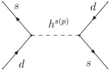
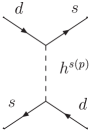
(a)	(b)

Figure 6: Feynman diagrams contributing to $\Delta m_{K}$ at tree-level.

From the interaction Lagrangians previously derived, it is now straightforward to compute the effective Hamiltonian for the diagrams in Fig. 6. One thus has $\mathcal{H}_{\text{eff}}=\mathcal{H}^{\sigma}_{\text{eff}}+\mathcal{H}^{\varphi}_{\text{eff}}$, with

$$\mathcal{H}^{\sigma}_{\text{eff}}= \operatornamewithlimits{\sum}_{\begin{smallmatrix}{j=1-6}\end{smallmatrix}}\frac{1}{16(m^{s}_{j})^{2}}\left\{\bar{s}\,\operatornamewithlimits{\sum}_{i=1,3,5}\left[({\mathcal{V}_{d}^{\dagger}}+\mathcal{V}_{d})^{ij}_{21}+({\mathcal{V}_{d}^{\dagger}}-\mathcal{V}_{d})_{21}^{ij}\gamma_{5}\right]d\right\}^{2}+\text{H.c.}\,,$$ (61)

$$\mathcal{H}^{\varphi}_{\text{eff}}= -\operatornamewithlimits{\sum}_{\begin{smallmatrix}{j=2-6}\end{smallmatrix}}\frac{1}{16(m^{p}_{j})^{2}}\left\{\bar{s}\,\operatornamewithlimits{\sum}_{i=1,3,5}\left[({\mathcal{W}_{d}}-\mathcal{W}_{d}^{\dagger})^{ij}_{21}-({\mathcal{W}_{d}}+\mathcal{W}_{d}^{\dagger})_{21}^{ij}\gamma_{5}\right]d\right\}^{2}+\text{H.c.}\,,$$ (62)

where the scalar and pseudoscalar Higgs masses, $m^{s,p}$, have been defined in Eq. (3.2). Therefore, the contribution to the kaon mass difference associated with the exchange of a scalar Higgs boson ($h^{s}$) is given by

$$\left.\mathcal{M}^{K}_{12}\right|^{\sigma}= \frac{1}{8}\operatornamewithlimits{\sum}_{\begin{smallmatrix}{j=1-6}\end{smallmatrix}}\frac{1}{(m^{s}_{j})^{2}}\left\{\left[\operatornamewithlimits{\sum}_{i=1,3,5}\left({\mathcal{V}_{d}}^{ij*}_{12}+{\mathcal{V}_{d}}^{ij}_{21}\right)\right]^{2}\langle\overline{K}^{0}\left|(\bar{s}d)(\bar{s}d)\right|K^{0}\rangle\right.$$

$$+\left.\left[\operatornamewithlimits{\sum}_{i=1,3,5}\left({\mathcal{V}_{d}}^{ij*}_{12}-{\mathcal{V}_{d}}^{ij}_{21}\right)\right]^{2}\langle\overline{K}^{0}\left|(\bar{s}\gamma_{5}d)(\bar{s}\gamma_{5}d)\right|K^{0}\rangle\right\}\,,$$ (63)

while the exchange of a pseudoscalar state ($h^{p}$) reads

$$\left.\mathcal{M}^{K}_{12}\right|^{\varphi}= \frac{1}{8}\operatornamewithlimits{\sum}_{\begin{smallmatrix}{j=2-6}\end{smallmatrix}}\frac{1}{(m^{p}_{j})^{2}}\left\{\left[\operatornamewithlimits{\sum}_{i=1,3,5}\left({\mathcal{W}_{d}}^{ij*}_{21}-{\mathcal{W}_{d}}^{ij}_{12}\right)\right]^{2}\langle\overline{K}^{0}\left|(\bar{s}d)(\bar{s}d)\right|K^{0}\rangle\right.$$

$$+\left.\left[\operatornamewithlimits{\sum}_{i=1,3,5}\left({\mathcal{W}_{d}}^{ij*}_{21}+{\mathcal{W}_{d}}^{ij}_{12}\right)\right]^{2}\langle\overline{K}^{0}\left|(\bar{s}\gamma_{5}d)(\bar{s}\gamma_{5}d)\right|K^{0}\rangle\right\}\,.$$ (64)

The theoretical prediction for the value of $\Delta m_{K}$ thus obtained should be compared with the experimental value of $(\Delta m_{K})_{\text{exp}}=3.49\times 10^{-12}$ MeV. We stress here that in a SM/MSSM-like scenario, the ${\mathcal{W}_{d}}$, ${\mathcal{V}_{d}}$ matrices entering in Eqs. (5.1, 5.1) would be diagonal in flavour space, and thus no tree-level FCNC would occur. This is clear from Eqs. (4), since the flavour content of $\mathcal{W}$ and $\mathcal{V}$ is proportional to $(V_{R}^{d}\,Y^{d}_{i}\,V^{d\dagger}_{L})_{ab}$. In the SM and MSSM, the matrices that diagonalise the quark mass matrices $V_{L,R}$ also diagonalise the Yukawa couplings, so $(V_{R}^{d}\,Y^{d}_{i}\,V^{d\dagger}_{L})_{ab}\propto\delta_{ab}$. In multi-Higgs doublet models, where the underlying theory implies that the Yukawas are proportional among themselves (i.e. $Y^{q}_{i}\propto Y^{q}_{j}$), we also encounter a situation where no tree-level FCNCs emerge.

Given the purpose of the analysis, we have adopted a simple approach regarding the computation of the meson matrix elements, using the vacuum insertion approximation with non-renormalised operators. Following Ref. [39], we have

$$\langle\overline{K}^{0}\left|(\bar{s}d)(\bar{s}d)\right|K^{0}\rangle =\left[\frac{1}{12}-\frac{1}{12}\left(\frac{m_{K}}{m_{s}+m_{d}}\right)^{2}\right]\,m_{K}\,f_{K}^{2}\,,$$

$$\langle\overline{K}^{0}\left|(\bar{s}\gamma_{5}d)(\bar{s}\gamma_{5}d)\right|K^{0}\rangle =\left[-\frac{1}{12}+\frac{11}{12}\left(\frac{m_{K}}{m_{s}+m_{d}}\right)^{2}\right]\,m_{K}\,f_{K}^{2}\,,$$ (65)

where $m_{K}$ is the kaon mass, and $f_{K}$ the kaon decay constant. In Table 1, we present several relevant input parameters for the computation of meson observables.

$m_{K}$	$497.6$ MeV	[38]	$m_{D^{0}}$	$1.864$ GeV	[38]
$\Delta m_{K}$	$3.49\times 10^{-12}$ MeV	[38]	$\Delta m_{D^{0}}$	$<46.07\times 10^{-12}$ MeV	[38]
$f_{K}$	$159$ MeV	[39]	$f_{D}$	$224$ MeV	[40]
$m_{B_{d}}$	$5.279$ GeV	[38]	$m_{B_{s}}$	$5.369$ GeV	[38]
$\Delta m_{B_{d}}$	$3.304\times 10^{-13}$ GeV	[38]	$\Delta m_{B_{s}}$	$>94.8\times 10^{-13}$ GeV	[38]
$f_{B_{d}}$	$215$ MeV	[41]	$f_{B_{s}}$	$245$ MeV	[41]

Table 1: Numerical values used throughout the computation with the corresponding references.

Before concluding the analysis of the neutral kaon sector, let us mention that in a scenario where one has flavour violating neutral Higgs couplings, and given the most generic possibility of having a complex CKM matrix, it is natural to expect the occurrence of indirect CP violation at the tree-level. Although we will not pursue this issue in the following numerical analysis, let us just stress that the contributions to $\varepsilon_{K}$ (which parametrises indirect CP violation in the kaon sector) are given by

$$\varepsilon_{K}=-\frac{e^{i\pi/4}}{\sqrt{2}}\,\frac{\operatorname{Im}\left[\mathcal{M}^{K}_{12}\lambda_{u}^{2}\right]}{|\lambda_{u}|^{2}\,\Delta m_{K}}\,,$$ (66)

where $\lambda_{u}$ is defined from CKM elements as $\lambda_{u}=V^{*}_{us}V_{ud}$, with $\mathcal{M}^{K}_{12}$ as computed in Eqs. (5.1,5.1) (under the assumption of complex Yukawa couplings). This new tree-level contribution would have to be compatible with the SM loop contribution and the experimental bound $\varepsilon_{K}=(2.284\pm 0.014)\times 10^{-3}$ [38].

5.2 Other neutral meson systems: $B_{d}$, $B_{s}$ and $D^{0}$

Computing the mass differences of neutral $B$ and $D$ mesons introduces no new elements into the analysis. The approach is entirely identical to that of the kaon system, the only difference lying in replacing the $K^{0}$ $(\bar{s}d)$ constituent quarks of Fig. 6 by $(\bar{u}c)$, $(\bar{b}d)$ and $(\bar{b}s)$, for $D^{0}$, $B_{d}$ and $B_{s}$, respectively. In each case the effective Hamiltonian for scalar and pseudoscalar Higgs exchange reads as in Eqs. (61, 62), providing that the following replacements are done:

$B_{d}$: $\mathcal{V}$ and $\mathcal{W}$ indices $(21)\to(31)$.

$B_{s}$: $\mathcal{V}$ and $\mathcal{W}$ indices $(21)\to(32)$.

$D$: $\mathcal{V}$ and $\mathcal{W}$ computed for the up-sector (see Eq. (4)); $\mathcal{V}$ and $\mathcal{W}$ indices $(21)\to(12)$; sum over interaction eigenstates $i=1,3,5\to i=2,4,6$.

In each case, the hadronic matrix elements should be also recomputed, and the predictions for each of the above processes should be confronted with the experimental data summarised in Table 1. Before concluding this section, let us briefly comment on the several observables mentioned here. First of all, it is widely recognised that, in models with tree-level FCNC, the most stringent bounds are usually associated with $\Delta m_{K}$. Regarding the $B_{d}$ sector, it has also been argued that in the absence of a predictive theory for the Yukawa couplings, the bounds associated with $\Delta m_{B_{d}}$ should be considered as a more reliable constraint, since they do not involve the mixing between the first two generations [19]. Although we include it in our analysis, the $B_{s}$ mass difference is not expected to add any new information. In the SM, this mixing is already maximal, and the addition of a new contribution would have little effect, the only exception occurring if new contributions matched exactly those of the SM, but had opposite sign, in which case a cancellation could take place. Still, this is a very fine-tuned scenario, and hardly significant, given the uncertainties associated with the computation. Finally, we turn our attention to the $D^{0}$ mass difference. As pointed out in [10, 13] and [42], models allowing for FCNC at the tree-level may present the possibility of very large contributions to $\Delta m_{D}$, thus emerging as an excellent probe of new physics effects. The latter contributions are often harder to control than those associated with, for example, $\Delta m_{K}$. In fact, and as discussed in [13], the contribution of tree-level FCNCs to $\Delta m_{D}$ could even exceed by a factor 20 those to $\Delta m_{K}$. On the other hand, mixing in the $D^{0}$ sector is very sensitive to the hadronic model used to estimate the transition amplitudes, and there is still a very large uncertainty in deriving its decay constants, etc. Therefore, the constraints on a given model arising from $\Delta m_{D}$ should not be over-emphasised.

Another interesting issue is that of rare decays. It has been argued that, again when no theory for the full Yukawas is available, some rare decays become very sensitive to flavour changing contributions induced by Higgs exchange at the tree-level. In Ref. [19], the authors have identified that the most promising decay modes involve the leptonic sector, together with the $B$-mesons, and are $\mu\to e\gamma$, $B_{d}\to K\mu\tau$ and $B_{s}\to\mu\tau$. We will not pursue this issue in the present work, reserving some of the above modes (namely $\mu\to e\gamma$) for a forthcoming analysis [43].

6 Flavour violation in six Higgs doublet models: results and discussion

6.1 Yukawa couplings: the simple Fritzsch scheme

We have carried out in the previous Section a general analysis of FCNC contributions. This can be applied to any particular model with three Higgs families, provided that the Yukawa couplings are known. Lead by simplicity, and following the analysis of [13], we take as an illustrative example the so-called “simple Fritzsch scheme” [31, 32]. Taking this ansatz for each of the Yukawa couplings presents two main advantages: it leads to mass matrices with a fairly hierarchical structure, and allows to fit experimental data on quark masses and mixings for a reasonable number of free parameters.

The “simple Fritzsch scheme” essentially consists in having all the weak quark eigenstates adopt identically structured couplings, which display suppressed flavour-changing elements for the first two generations in each family. More explicitly one has

$$Y_{i}\,=\,\frac{1}{w_{i}}\,\left(\begin{array}[]{ccc}0&A_{i}&0\\ A_{i}&0&B_{i}\\ 0&B_{i}&C_{i}\end{array}\right)\,,$$ (70)

where $i=1,...,6$, and the entries are given by

$$A_{i}=a_{i}\,\sqrt{m_{1}^{q}\,m_{2}^{q}}\,,\quad\quad B_{i}=b_{i}\,\sqrt{m_{2}^{q}\,m_{3}^{q}}\,,\quad\quad C_{i}=c_{i}\,m_{3}^{q}\,,$$ (71)

with $a_{i}$, $b_{i}$ and $c_{i}$ coefficients of order one, and $m^{q}_{j}$ the quark masses of the $j^{\text{th}}$ generation and $q=d\,(u)$ for $i=1,3,5\,(2,4,6)$. One further advantage of this choice, which will become more evident in the subsequent discussion, is that under the above ansatz, the quark masses and mixings are independent of the chosen VEV regime (although the Yukawas are not). This means that for a given successful choice of the parameters $a_{i}$, $b_{i}$ and $c_{i}$, one can study a number of distinct VEV schemes, corresponding to different $\tan\beta$ scenarios.

Let us now present a specific numerical example. Taking the values for the input quark masses, $m_{i}^{q}$ entering in the ansatz of Eq. (71) as $m_{u}=3$ MeV, $m_{d}=6.5$ MeV, $m_{c}=1.25$ GeV, $m_{s}=0.1$ GeV, $m_{t}=178$ GeV, $m_{b}=$4.5 GeV, and using the following choice of coefficients

$$a\,=\,\{0.45,0.30,0.35,0.45,0.20,0.50\}\,,$$

$$b\,=\,\{0.25,0.40,0.45,0.30,0.20,0.35\}\,,$$

$$c\,=\,\{0.30,0.45,0.30,0.30,0.40,0.25\}\,,$$ (72)

one obtains the following set of output quark masses

$$m_{u}=0.0042\,\,\text{GeV}\,,\quad m_{c}=1.37\,\,\text{GeV}\,,\,\quad m_{t}=179.4\,\,\text{GeV}$$

$$m_{d}=0.0073\,\,\text{GeV}\,,\quad m_{s}=0.087\,\,\text{GeV}\,,\quad m_{b}=4.5\,\,\text{GeV}$$ (73)

and the associated mixing matrix

$$\left|V_{\text{CKM}}\right|\,=\,\left(\begin{array}[]{ccc}0.9742&0.2255&0.0031\\ 0.2251&0.9733&0.0438\\ 0.0129&0.0420&0.9990\end{array}\right)\,,$$ (74)

which is in good agreement with experimental data. Having the relevant data (Yukawa couplings and CKM matrix), we can now proceed to estimate the contributions to neutral meson mass differences. As stressed before, we are considering a general multi-Higgs model, so that we have no definite scheme for the $\mu$-terms and soft SUSY breaking masses. Therefore, and as done in Section 2, we will assume simple textures for the Higgs sector.

6.2 Tree-level FCNC in neutral mesons: numerical results

The first step in evaluating the contributions to tree-level FCNC is to parameterise the Higgs sector, and thus obtain the mixing matrices and mass eigenstates entering in Eqs. (5.1,5.1). As discussed in Section 2, the Higgs basis is far more intuitive to work in than the original superpotential basis. Working in Higgs-basis notation (see Eqs. (14-28)), let us assume that the free parameters $m^{2}_{ij}$ and $b_{ij}$ obey the following simple patterns:

$$m^{(d)}_{ij}=\left(\begin{array}[]{ccc}{\otimes}&{\otimes}&{\otimes}\\ {\otimes}&x_{3}&y\\ {\otimes}&y&x_{5}\end{array}\right)\times{1\text{TeV}}\,,\quad m^{(u)}_{ij}=\left(\begin{array}[]{ccc}{\otimes}&{\otimes}&{\otimes}\\ {\otimes}&x_{4}&y\\ {\otimes}&y&x_{6}\end{array}\right)\times{1\text{TeV}}\,,\quad\sqrt{b_{ij}}=\sqrt{b}\times{1\text{TeV}}\,,$$ (81)

where the $\otimes$ denotes an entry which is fixed by the minimisation conditions (cf. Eqs. (2.2,2.2)). The above parametrisation can be further simplified by taking $x_{3}=x_{4}$ and $x_{6}=x_{5}$. Therefore, we have the following free parameters associated with the Higgs sector:

$$x_{3}\,,\quad x_{5}\,,\quad\sqrt{b}\,,\quad\tan\beta\,,$$ (82)

and the pattern of VEVs, namely whether they are degenerate or hierarchical. In the numerical examples we will thus consider the following textures for $m^{2}_{ij}$ and $b_{ij}$.

$$\text{(A)}\,:\quad \quad x_{3}=1\,,\quad x_{5}=5\,,\quad y=0.4\,,\quad\sqrt{b}=0.3\,,$$

$$\text{(B)}\,:\quad \quad x_{3}=10\,,\quad x_{5}=10\,,\quad y=0.6\,,\quad\sqrt{b}=0.5\,.$$ (83)

In each case, we will consider several values for $\tan\beta$, taking it to lie in the range $3\lesssim\tan\beta\lesssim 12$. Moreover, for every $\tan\beta$ we take to very distinct schemes of VEVs, that while respecting the EW symmetry breaking conditions and being in agreement with the chosen $\tan\beta$ value, exhibit either a degenerate pattern ($w_{1}=w_{3}=w_{5}$, $w_{2}=w_{4}=w_{6}$) or a strongly hierarchical one ($w_{5}=10\,w_{3}=100\,w_{1}$, $w_{6}=10\,w_{4}=100\,w_{2}$).

For the above range of $\tan\beta$, the Higgs spectra (lightest and heaviest scalar, pseudoscalar and charged states) is within the following ranges :

$$\text{Texture \ (A)}:$$

$$79\,\text{GeV}\lesssim m_{1}^{s}\lesssim 90\,\text{GeV}\,,\quad 198\,\text{GeV}\lesssim m_{2}^{p}\lesssim 409\,\text{GeV}\,,\quad 417\,\text{GeV}\lesssim m_{2}^{\pm}\lesssim 203\,\text{GeV}\,,$$

$$\quad\quad\quad\quad\quad\quad 5009\,\text{GeV}\lesssim m_{6}^{s},\ m_{6}^{p},\ m_{5}^{\pm}\lesssim 5011\,\text{GeV}\,.$$

$$\text{Texture \ (B)}:$$

$$79\,\text{GeV}\lesssim m_{1}^{s}\lesssim 90\,\text{GeV}\,,\quad 908\,\text{GeV}\lesssim m_{2}^{p}\lesssim 1547\,\text{GeV}\,,\quad 909\,\text{GeV}\lesssim m_{2}^{\pm}\lesssim 1549\,\text{GeV}\,,$$

$$\quad\quad\quad\quad\quad\quad 10043\,\text{GeV}\lesssim m_{6}^{s},\ m_{6}^{p},\ m_{5}^{\pm}\lesssim 10047\text{GeV}\,.$$ (84)

Let us begin by addressing the observable which is associated to most stringent constraints for this class of models: $\Delta m_{K}$. In Fig. 7, we plot ratio $\Delta m_{K}/(\Delta m_{K})_{\text{exp}}$ as a function of $\tan\beta$ for textures (A) and (B), considering in each case a pattern of degenerate (Deg) or non-degenerate (NDeg) VEVs.

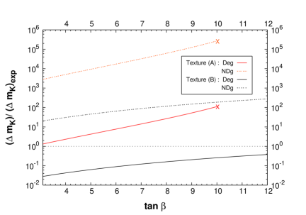
Figure 7: $\Delta m_{K}/(\Delta m_{K})_{\text{exp}}$ as a function of $\tan\beta$. Full (dashed) red line denotes texture (A) for degenerate (hierarchical) VEVs, while a black full (dashed) line refers to texture (B) with degenerate (hierarchical) VEVs. For Texture (A) a cross marks the appearance of tachyonic states. The experimental bound is depicted via a dotted horizontal line.

Fig. 7 clearly reflects the most problematic aspect of this class of multi-Higgs doublet models. Without a symmetry forbidding some of the Yukawa couplings, and if the Yukawas themselves do not exhibit a strong hierarchical character, the contributions to the neutral kaon mass difference can only be brought down to the experimental value via a set of very heavy Higgses, as those of texture (B). A Higgs spectrum closer to the EW scale, with a typical mass scale of 500 GeV, would generate, for the case of degenerate (non-degenerate) VEVs, contributions to $\Delta m_{K}$ of around 30 ($3\times 10^{4}$) $(\Delta m_{K})_{\text{exp}}$. It is also manifest that smaller values of $\tan\beta$ favour smaller contributions. This is due to having the Yukawa couplings for the down quarks proportional to $\sec\beta$. The relevance of the VEV regime should also be emphasised, since the latter plays a very important role. Even though the Yukawas enter in the contribution to $\mathcal{M}_{12}^{K}$ already rotated by the matrices that diagonalise the quark mass matrices, it is clear that the smaller the VEVs associated to the first and second quark generations, the more enhanced will be the (12) matrix elements. In the case of degenerate VEVs, all the Yukawas are identically suppressed/enhanced. Naturally, assuming such a large scale for the soft-breaking terms potentially leads to a fine tuning problem. As pointed out in Section 2.3, and even though the discussion was conducted for a distinct basis, masses above the few TeV scale are in principle within range of a more than 1% fine tuning.

When compared to some previous studies, our results are more severe. However, let us stress that in our analysis we have taken a few distinct steps. Firstly, and in comparison to the ansätze used in [13], our Yukawa couplings are quite different, since accommodating the current CKM matrix data leads to values of $a_{i},\,b_{i}$ and $c_{i}$ quite smaller than those previously considered. This implies that the present Yukawas are less hierarchic. Moreover, we have explicitly taken into account the values of the VEVs, and considered the contributions from the exchange of all physical scalar and pseudoscalar Higgses (not weak interaction eigenstates), taking into account not only their masses, but also their mixings. It is also important to mention that the values of the hadronic matrix elements have been revised in the past years.

In Fig. 8, we present the contributions to the mass difference of the $B_{d}$ mesons. As expected, in this case it is far easier to comply with the experimental bounds.

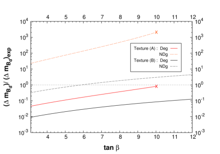
Figure 8: $\Delta m_{B_{d}}/(\Delta m_{B_{d}})_{\text{exp}}$ as a function of $\tan\beta$. Line and colour codes as in Fig. 7.

For the case of degenerate VEVs, even the “lightest” texture (A) succeeds in complying with the experimental bounds throughout the whole range of $\tan\beta$ considered, while for the heavier Higgs set (B), with non-degenerate VEVs. compatibility is obtained for the low $\tan\beta$ regime ($\tan\beta\lesssim 6$).

To complete our study, we display in Fig. 9 the same analysis for the case of the $B_{s}$ meson system. In this case, the experimental bound is a lower (rather than upper bound).

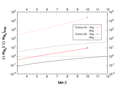
Figure 9: $\Delta m_{B_{s}}/(\Delta m_{B_{s}})_{\text{exp}}$ as a function of $\tan\beta$. Line and colour codes as in Fig. 7.

As discussed in Section 5, the SM already has maximal mixing in the $B_{s}$ system, and even though the new contributions may be of identical magnitude, there is no reason to expect a cancellation between SM and tree-level contributions, which would be associated to an extremely fine tuned scenario for all the parameters involved.

From the meson systems so far discussed, the most severe constraints arise, as expected, from the $K_{L}-K_{S}$ mass difference. As a final remark, and following the discussion of Section 5, we briefly comment on the predicted scenario involving the $D^{0}$ mesons. A study similar to those conducted for the $K^{0}$ and $B$ sectors is of less interest, since there is little dependence of $\Delta m_{D}/(\Delta m_{D})_{\text{exp}}$ on $\tan\beta$. This is due to having the up-type quarks Yukawa couplings associated to $\csc\beta$, as seen from Eq. (70).

Rather than presenting a plot, we will briefly summarise the situation. With the exception of Texture (A), with non-degenerate VEVs, which induces contributions to $\Delta m_{D}$ around 10 times its experimental value, all other cases predict contributions below the experimental bound, ranging from $10^{-3}$ to $10^{-1}$ $(\Delta m_{D})_{\text{exp}}$.

To summarise, ansätze for the Yukawa couplings of the “simple Fritzsch” type, when generalised to multi-Higgs doublet models, typically induce tree-level FCNC’s, and require a Higgs spectrum at least of order 10 TeV, in order to ensure compatibility with experiment. Notice however that the results presented here are very dependent on the assumed scheme for the Yukawa couplings, and are only to be taken as an illustrative example, in the absence of a full theory for the Higgs-quark-quark interactions. Predictive models for Yukawa interactions of extended Higgs sector are likely to account for distinct, and hopefully less severe, bounds [7].

7 Conclusions

Models that predict family replication in the Higgs sector offer a very aesthetic and phenomenologically interesting scenarios. Although there is abundant motivation for extending the Higgs sector (from string constructions, for example), in most cases the viability of these models is challenged by the occurrence of potentially dangerous FCNCs at the tree-level.

We have analysed the most general form of the SUSY potential with three Higgs families, studying its minimisation, and deriving the tree-level expressions for the neutral (scalar and pseudoscalar) and charged Higgses mass matrices.

The main goal of our work was to derive a model-independent evaluation of the tree-level contributions to neutral meson mass differences. We have computed the most general expression for the tree-level neutral Higgs mediated contributions to the mass difference of the neutral mesons. We took into account the exchange of all Higgs states, included the effects of mixing in the Higgs sector, and made no approximation with respect to dominant/sub-dominant contributions. This analysis is completely general, and can be applied to any given model with three Higgs families, independently of its Yukawa structure. As an example, in Section 6 we have assumed a simple ansatz for the Yukawa couplings (in analogy to what had previously been done), and have considered the contributions of two distinct Higgs spectra to the $K^{0}$, $B_{d}$, $B_{s}$ and $D^{0}$ mass differences, finding that the strongest bound - which as expected arises from $\Delta m_{K}$ - requires a spectrum of order 10 TeV.

We again remark that the results for the Higgs masses are strongly dependent on the specific ansatz for the Yukawa couplings. Other ansätze, that account for a stronger hierarchy in the quark sector and still accommodate experimental data on quark masses and mixings, may generate quite smaller contributions to $\Delta m_{K}$, and thus require a lighter Higgs spectrum. This possibility is the subject of a forthcoming work [7], where it is shown that a Higgs spectra of order 1 TeV can be accommodated. On the other hand, it is also possible that while generating smaller contributions to $\Delta m_{K}$, the different ansätze induce larger $\Delta m_{B}$, or $\Delta m_{D}$.

In addition to the contributions to neutral meson mass difference, within the quark sector there are other processes that also deserve further investigation. For example, let us mention, at the one loop level, the very suppressed SM and MSSM $B_{s}$ decays. Processes involving the lepton sector also offer an even wider field for testing the new contributions induced by the additional Higgses (neutral and charged) [43]. CP violation, given the potential tree-level contributions to $\varepsilon_{K}$, may also become a stringent bound.

References

- [1] D. J. Gross, J. A. Harvey, E. Martinec and R. Rohm, “The heterotic string”, Phys. Rev. Lett. 54 (1985) 502.
- [2] J. A. Casas and C. Muñoz, “Three generation SU(3) SU(2) U(1)Y U(1) orbifold models through Fayet-Iliopoulos terms”, Phys. Lett. B 209 (1988) 214.
- [3] J. A. Casas and C. Muñoz, “Three generation SU(3) SU(2) U(1)Y models from orbifolds”, Phys. Lett. B 214 (1988) 63.
- [4] A. Font, L. E. Ibáñez, F. Quevedo and A. Sierra, “The construction of ’realistic’ four dimensional strings through orbifolds”, Nucl. Phys. B 331 (1990) 421.
- [5] C. Muñoz, “A kind of prediction from superstring model building”, JHEP 0112 (2001) 015 [arXiv:hep-ph/0110381].
- [6] S. A. Abel and C. Muñoz, “Quark and lepton masses and mixing angles from superstring constructions,” JHEP 0302 (2003) 010 [arXiv:hep-ph/0212258].
- [7] N. Escudero, C. Muñoz and A. M. Teixeira, “Phenomenological viability of orbifold models with three Higgs families”, in preparation.
- [8] See, for example, G. Aldazabal, L. E. Ibáñez, F. Quevedo and A. M. Uranga, “D-branes at singularities: a bottom-up approach to the string embedding of the standard model”, JHEP 0008 (2000) 002 [arXiv:hep-th/0005067].
- [9] H. Georgi and D. V. Nanopoulos, “Suppression of flavor changing effects from neutral spinless meson exchange in gauge theories”, Phys. Lett. B 82 (1979) 95.
- [10] B. McWilliams and L. F. Li, “Virtual effects of Higgs particles”, Nucl. Phys. B 179 (1981) 62.
- [11] O. Shanker, “Flavor violation, scalar particles and leptoquarks”, Nucl. Phys. B 206 (1982) 253.
- [12] R. A. Flores and M. Sher, “Higgs masses in the standard, multi - Higgs and supersymmetric models”, Annals Phys. 148 (1983) 95.
- [13] T. P. Cheng and M. Sher, “Mass matrix ansatz and flavor nonconservation in models with multiple Higgs doublets”, Phys. Rev. D 35 (1987) 3484.
- [14] J. R. Ellis, D. V. Nanopoulos, S. T. Petcov and F. Zwirner, “Gauginos and Higgs particles in superstring models”, Nucl. Phys. B 283 (1987) 93.
- [15] M. Drees, “Supersymmetric models with extended Higgs sector,” Int. J. Mod. Phys. A 4 (1989) 3635.
- [16] K. Griest and M. Sher, “Phenomenology and cosmology of extra generations of Higgs bosons”, Phys. Rev. Lett. 64 (1990) 135.
- [17] K. Griest and M. Sher, “Phenomenology and cosmology of second and third family Higgs bosons”, Phys. Rev. D 42 (1990) 3834.
- [18] H. E. Haber and Y. Nir, “Multiscalar models with a high-energy scale”, Nucl. Phys. B 335 (1990) 363.
- [19] M. Sher and Y. Yuan, “Rare B decays, rare tau decays and grand unification”, Phys. Rev. D 44 (1991) 1461.
- [20] N. V. Krasnikov, “Electroweak model with a Higgs democracy”, Phys. Lett. B 276 (1992) 127.
- [21] A. Antaramian, L. J. Hall and A. Rasin, “Flavor changing interactions mediated by scalars at the weak scale”, Phys. Rev. Lett. 69 (1992) 1871 [arXiv:hep-ph/9206205].
- [22] A. E. Nelson and L. Randall, “Naturally large tan beta”, Phys. Lett. B 316 (1993) 516 [arXiv:hep-ph/9308277].
- [23] M. Masip and A. Rasin, “Spontaneous CP violation in supersymmetric models with four Higgs doublets”, Phys. Rev. D 52 (1995) R3768 [arXiv:hep-ph/9506471].
- [24] M. Masip and A. Rasin, “CP violation in multi-Higgs supersymmetric models”, Nucl. Phys. B 460 (1996) 449 [arXiv:hep-ph/9508365].
- [25] A. Aranda and M. Sher, “Generations of Higgs bosons in supersymmetric models”, Phys. Rev. D 62 (2000) 092002 [arXiv:hep-ph/0005113].
- [26] S. Béjar, J. Guasch and J. Solà, “Production and FCNC decay of supersymmetric Higgs bosons into heavy quarks in the LHC”, JHEP 0510 (2005) 113 [arXiv:hep-ph/0508043].
- [27] A. M. Curiel, M. J. Herrero, W. Hollik, F. Merz and S. Peñaranda, “SUSY - electroweak one-loop contributions to flavour-changing Higgs-boson decays”, Phys. Rev. D 69 (2004) 075009 [arXiv:hep-ph/0312135].
- [28] J. A. Aguilar-Saavedra, “Top flavour-changing neutral interactions: Theoretical expectations and experimental detection”, Acta Phys. Polon. B 35 (2004) 2695 [arXiv:hep-ph/0409342].
- [29] S. L. Glashow and S. Weinberg, “Natural conservation laws for neutral currents”, Phys. Rev. D 15 (1977) 1958.
- [30] E. A. Paschos, “Diagonal neutral currents”, Phys. Rev. D 15 (1977) 1966.
- [31] H. Fritzsch, “Weak interaction mixing in the six - quark theory”, Phys. Lett. B 73 (1978) 317.
- [32] H. Fritzsch and Z. z. Xing, “Mass and flavor mixing schemes of quarks and leptons”, Prog. Part. Nucl. Phys. 45 (2000) 1 [arXiv:hep-ph/9912358].
- [33] W. K. Sze, “The Fritzsch ansatz revisited”, arXiv:hep-ph/0511181.
- [34] For a review see, A. Brignole, L. E. Ibáñez and C. Muñoz, “Soft supersymmetry-breaking terms from supergravity and superstring models”, in the book “Perspectives on supersymmetry”, G. L. Kane (ed.), World Scientific (1998) 125 [arXiv:hep-ph/9707209].
- [35] R. Barbieri and G. F. Giudice, “Upper bounds on supersymmetric particle masses”, Nucl. Phys. B 306 (1988) 63.
- [36] J. A. Casas, J. R. Espinosa and I. Hidalgo, “Implications for new physics from fine-tuning arguments. I: Application to SUSY and seesaw cases”, JHEP 0411 (2004) 057 [arXiv:hep-ph/0410298].
- [37] Y. Sakamura, “The Higgs mass bound in the SUSY multi-Higgs-doublet model”, Mod. Phys. Lett. A 14 (1999) 721 [arXiv:hep-ph/9903247].
- [38] S. Eidelman et al. [Particle Data Group Collaboration], “Review of particle physics”, Phys. Lett. B 592 (2004) 1.
- [39] M. Ciuchini et al., “Delta M(K) and epsilon(K) in SUSY at the next-to-leading order”, JHEP 9810, 008 (1998) [arXiv:hep-ph/9808328].
- [40] J. N. Simone et al. [The Fermilab Lattice, MILC and HPQCD Collaborations], “Leptonic decay constants f(D/s) and f(D) in three flavor lattice QCD”, Nucl. Phys. Proc. Suppl. 140 (2005) 443 [arXiv:hep-lat/0410030].
- [41] S. Aoki et al. [JLQCD Collaboration], “B0 anti-B0 mixing in unquenched lattice QCD”, Phys. Rev. Lett. 91 (2003) 212001 [arXiv:hep-ph/0307039].
- [42] G. Burdman, “Potential for discoveries in charm meson physics”, arXiv:hep-ph/9508349.
- [43] N. Escudero, C. Muñoz and A. M. Teixeira, work in progress.