Non-minimal models of supersymmetric spontaneous CP violation

Abstract

We briefly review the question of spontaneous CP violation in some models of weak interactions. The next-to-minimal supersymmetric standard model, with two Higgs doublets and one gauge singlet, is one of the minimal extensions of the standard model where SCPV is viable. We analyse the possibility of spontaneous CP violation the next-to-minimal supersymmetric standard model with an extra singlet tadpole term in the scalar potential, and confirm the existence of phenomenologically consistent minima with non-trivial CP violating phases.

11.30.Er, 11.30.Qc, 12.60.Jv

1 Introduction

The origin and realisation of the breaking of the CP symmetry in nature remains an illusive topic in modern particle physics [1] . Although the standard model of particle physics (SM) succeeds in accommodating the experimentally observed values of CP violation (CPV) in meson physics though the Cabbibo-Kobayashi-Maskawa mechanism, many questions remain to be answered. Among the most relevant issues are the explanation of the observed baryon asymmetry of the Universe (which requires new sources of CPV from physics beyond the SM), and the strong CP problem. The strong CP problem, or equivalently, the smallness of the $\bar{\theta}$ parameter, is the source of an important SM fine-tuning problem. In fact, experimental bounds from the electric dipole moment (EDM) of the electron, neutron and mercury atom force the flavour conserving phase $\bar{\theta}$ to be as small as $10^{-10}$, a most unnatural value in the sense of ’t Hooft [2], since the SM Lagrangian does not acquire a new symmetry in the limit where $\bar{\theta}\to 0$.

In the SM, CP violation is implemented in an explicit way: the presence of complex Yukawa couplings breaks the CP symmetry at Lagrangian level. However, this is not the only mechanism of CP violation. A second and very attractive possibility lies in spontaneous CP violation (SCPV), a framework where CP is originally a symmetry of the Lagrangian, which is dynamically broken by complex scalar vacuum expectation values (VEVs).

The scenario of SCPV (or soft CPV), originally proposed by T. D. Lee [3], is based on the follow principles: originally, the Lagrangian describing the $SU(2)_{L}\times U(1)_{Y}$ theory is invariant under a transformation that one can associate with the CP symmetry. During the process of electroweak (EW) symmetry breaking, the scalar field that is responsible for the breaking $SU(2)_{L}\times U(1)_{Y}\to U(1)_{\mathrm{em}}$ acquires a complex VEV, so that after EW symmetry breaking the Lagrangian is not longer CP invariant. The effects of SCPV are finite in renormalisable theories [3].

The motivations for SCPV are extensive, and the strongest are related with providing a solution to the strong CP problem, as well as establishing a connection between the breaking of the CP symmetry at very high energies (where it could be understood in the framework of some fundamental theory of particle physics - string theory, for instance) and low energy phenomenology. Regarding the strong CP problem, if CP is imposed as a symmetry of the Lagrangian prior to spontaneous EW symmetry breaking, at the tree-level one directly obtains $\bar{\theta}=0$. Within the context of supersymmetric (SUSY) theories, SCPV emerges as a natural candidate to explain the SUSY CP-problem. SUSY models as the minimal supersymmetric standard model (MSSM) introduce a vast array of new CP violating phases, some of them flavour-conserving (as those associated with the $\mu$-term and the soft gaugino masses). These phases also generate sizable contributions to the EDMs, and are forced to be very small to ensure compatibility with experiment, leading to another naturalness problem - the SUSY CP-problem. Under SCPV, all these phases are set to zero at some intermediate scale via the imposition of a symmetry, which is then softly broken, thus allowing to evade ’t Hooft’s criteria [4]. Further motivation for SCPV stems from string theory, where it has been shown that in string perturbation theory CP exists as a symmetry that could be spontaneously broken. In this framework, CP violation could be induced by non-trivial properties of the manifold, or by CP non-invariant compactification boundary conditions. Alternatively, CPV could also originate from complex VEVs of the moduli fields. It has also been argued that CP can be a gauge symmetry in string theory [5], which is spontaneously broken at a high scale, the effects then being fed to the Yukawa couplings in the superpotential, and to the soft breaking terms.

Effective low energy models with a minimal Higgs field content, as is the case of the SM, are not viable scenarios for SCPV. In fact, SCPV requires at least two Higgs doublets, as is the case of the Lee model. Supersymmetric models emerge as interesting candidate scenarios for SCPV. Not only one has at least a minimal content of two Higgs doublets, but as discussed before, SCPV also solves issues as the SUSY CP-problem. In section 2 we shall present a short overview of SCPV in SUSY scenarios. In section 3, we focus our discussion in the specific case of the next-to-minimal supersymmetric standard model with a $\mathbb{Z}_{3}$ symmetry in the superpotential [21], and an additional tadpole term in the scalar potential. After defining the model, we address the minimisation of the scalar potential, and study the mass spectrum. Finally, in section 4, we consider the contributions to indirect CP violation in the neutral Kaon sector (parametrised by $\varepsilon_{K}$), and present our numerical results. A summarising outlook is presented in the Conclusions.

2 Models of SUSY spontaneous CP violation

Even though the original Lee model appeared to encompass all the necessary ingredients for minimally extending the SM in order to arrive at an electroweak model that softly broke CP, many were the phenomenological problems that plagued it. Among them were excessive contributions to leptonic and nucleon EDMs, and most important, the existence of flavour-changing neutral Yukawa interactions (FCNYI). FCNYI are a usual feature of multi-Higgs doublet models, and typically induce excessive (and experimentally incompatible) contributions to neutral meson mixing and rare decays. The most elegant way to suppress them is to assume the existence of some underlying mechanism (a symmetry) that removes the dangerous Higgs-quark couplings. As shown in [6], the only way to have natural flavour conservation is by imposing that each of the scalar doublets only couples to a quark of a given charge. This can be achieved by imposing a number of discrete symmetries on the Lagrangian. Albeit, once such symmetries are imposed, SCPV in no longer possible.

One can further increase the number of the Higgs doublets: in the Branco model [7], which contains three doublets and has natural flavour conservation, CP can be spontaneously broken and scalar particle interactions are the only source of CP violation. One should also mention that SCPV can also occur in models where, instead of just enlarging the Higgs sector, one has additional fermions or an extended gauge sector (e.g. extended left-right symmetric models, models with additional heavy exotic fermions, vector-like quark models - see [1] for a comprehensive review).

The MSSM emerges as an appealing scenario for SCPV, since it has by construction two Higgs doublets, and natural flavour conservation is automatic. Nevertheless, it is well known that, at the tree-level, SCPV does not occur in the MSSM [8]. On the other hand, radiative corrections can generate CP violating operators [9] but then, according to the Georgi-Pais theorem on radiatively broken global symmetries [10], one expects to have light states in the Higgs spectrum [11], which are excluded by LEP [12, 13, 14]. Thus, it is of interest to consider simple extensions of the MSSM, such as a model with at least one gauge singlet field ($N$) in addition to the two Higgs doublets - the so-called the next-to-minimal supersymmetric standard model (NMSSM), and investigate whether SCPV can be achieved in this class of models.

The NMSSM [15] is a particularly appealing SUSY model, since it allows to solve another MSSM naturalness problems, the so-called $\mu$ problem [16]. The $\mu$ problem arises from the presence of a mass term for the Higgs fields in the superpotential, $\mu H_{1}H_{2}$. The only natural values for the $\mu$ parameter are either zero or the Planck scale. The first is experimentally excluded, since it leads to an unacceptable axion once the EW symmetry is broken. The second is equally unpleasant, since it reintroduces the hierarchy problem. Although there are several explanations for an $\mathcal{O}(M_{W})$ value for the $\mu$ term, all are in extended frameworks. The NMSSM offers a simple yet elegant solution via the presence of a trilinear dimensionless coupling in the superpotential, $\lambda NH_{1}H_{2}$. When the scalar component of $N$ acquires a VEV of the order of the SUSY breaking scale, an effective $\mu$ term is dynamically generated. This realisation of the NMSSM, where the superpotential is invariant under a $\mathbb{Z}_{3}$ symmetry is the simplest SUSY extension of the SM where the EW scale exclusively originates from SUSY breaking.

From the point of view of SCPV, and in spite of all its many attractive features, the NMSSM presents some problems. It has been shown that in the simplest $\mathbb{Z}_{3}$ invariant version, there is no SCPV at the tree-level. Even though CP violating extrema can be found, these are maxima, and not minima of the potential, associated with tachyonic Higgs states (no-go theorem) [17]. Regarding the possiblity of radiatively induced SCPV in the $\mathbb{Z}_{3}$ symmetric NMSSM, the situation is very similar to the MSSM case, since the CPV minima are associated to very light Higgs states, which are difficult to accomodate with experimental data [18, 19].

If one abandons the prospect of solving the $\mu$ problem, and allows the presence of dimensionfull, SUSY conserving terms in the superpotential, SCPV is indeed viable. As shown in [20, 21], one can find CP violating minima of the potential which are in agreement with experimental data on the Higgs sector, and can successfully account for the observed value of $\varepsilon_{K}$. However, these models encompass an important theoretical drawback, since in the absence of a global symmetry under which the singlet field is charged, divergent singlet tadpoles proportional to $M_{\mathrm{Planck}}$, generated by non-renormalizable higher order interactions, can appear in the effective scalar potential [22]. These would lead to a destabilisation of the hierarchy between EW the Planck scale. On the other hand, imposing a discrete symmetry to overcome the latter problem leads to disastrous cosmological domain walls

Still, there is a possible solution to this controversial puzzle, which consists in finding NMSSM models that while $\mathbb{Z}_{3}$-violating, have a $\mathbb{Z}_{3}$ conserving superpotential. As pointed out in [23], using global discrete $R$-symmetries for the complete theory - including non-renormalisable interactions - one could construct a $\mathbb{Z}_{3}$ invariant renormalisable superpotential and generate a $\mathbb{Z}_{3}$ breaking non-divergent singlet tadpole term in the scalar potential. In addition to being free of both stability and domain wall problems, these models present a rather unique feature: they are a viable scenario for SCPV, where one can obtain the observed value of $\varepsilon_{K}$, and have at the same time compatibility with experimental data [24]. In the following section we proceed to analyse this class of models in greater detail.

3 Spontaneous CP violation in the NMSSM

In this section, we will address the possibility of SCPV in the NMSSM with an extra singlet tadpole term in the effective potential, taking into account the constraints on Higgs and sparticle masses. We begin by briefly describing the model, focusing of the Higgs scalar potential and its minimisation. We then proceed to compute the masses of the Higgs states, including radiative corrections, and present a short numerical analysis of the neutral Higgs spectrum.

3.1 The scalar Higgs potential

We consider the most general form of the superpotential where, in addition to the Yukawa couplings for quark and leptons (as in the MSSM), we have the following Higgs couplings

$$W_{\mathrm{Higgs}}=\lambda\hat{H}_{1}\hat{H}_{2}\hat{N}+\frac{1}{3}\kappa\hat{N}^{3}\;,$$ (1)

where $\hat{N}$ is a singlet superfield, and $H_{1,2}$ are the usual MSSM HIggs doublets. After EW symmetry breaking, the scalar component of $\hat{N}$ acquires a VEV, $x=|\langle N\rangle|$, thus generating an effective $\mu$ term

$$\mu\equiv\lambda x\;.$$ (2)

As mentioned in the previous section, a possible means to overcome the domain wall problem without spoiling the quantum stability of the model is by replacing the $\mathbb{Z}_{3}$ symmetry by a set of discrete $R$-symmetries, broken by the soft SUSY breaking terms [23]. At low energy, the additional non-renormalisable terms allowed by the $R$-symmetries generate an extra linear term for the singlet in the effective potential, through tadpole loop diagrams

$$V_{\mathrm{tadpole}}=-\xi^{3}N+\mathrm{H.c.}\;,$$ (3)

where $\xi$ is of the order of the soft SUSY breaking terms ($\lesssim$ 1 TeV). In addition to $V_{\mathrm{tadpole}}$ the tree-level Higgs potential comprises the usual $D-$ and $F$-terms, as well as soft-SUSY breaking interactions. The latter are given by

$$V_{\mathrm{soft}}=m_{H_{i}}^{2}|H_{i}|^{2}+m_{N}^{2}|N|^{2}+\left(\lambda A_{\lambda}NH_{1}H_{2}+\frac{1}{3}\kappa A_{\kappa}N^{3}+\mathrm{H.c.}\right).$$ (4)

In the above, we take the soft-SUSY breaking terms $m_{H_{1}},m_{H_{2}},m_{N},A_{\lambda},A_{\kappa}$ as free parameters at the weak scale. We also assume that the Lagrangian is CP invariant, which means that all the parameters appearing in Eqs. (3,4) are real.

After spontaneous EW symmetry breaking, the neutral Higgses acquire complex VEVs that spontaneously break CP:

$$\langle H_{1}^{0}\rangle=v_{1}e^{i\varphi_{1}}\;,\quad\langle H_{2}^{0}\rangle=v_{2}e^{i\varphi_{2}}\;,\quad\langle N\rangle=xe^{i\varphi_{3}}\;,$$ (5)

where $v_{1},v_{2},x$ are positive and $\varphi_{1},\varphi_{2},\varphi_{3}$ are CP violating phases. However, only two of these phases are physical. They can be chosen as

$$\theta=\varphi_{1}+\varphi_{2}+\varphi_{3}\quad\mathrm{and}\quad\delta=3\varphi_{3}\;.$$ (6)

3.2 CP violating minima of the scalar potential

From the tree-level scalar potential of Eqs.3,4), together with the associated $D$- and $F$- terms (see [24]), one can derive the five minimisation equations for the VEVs and phases $v_{1},v_{2},x,\theta,\delta$. These can be used to express the soft parameters $m_{H_{1}},m_{H_{2}}$, $m_{N},A_{\lambda},A_{\kappa}$ in terms of $v_{1},v_{2},x,\theta,\delta$:

$$\frac{\partial V_{\mathrm{tree}}}{\partial v_{1}}=0\quad\Rightarrow\quad m_{H_{1}}^{2} = -\lambda^{2}\left(x^{2}+v^{2}\sin^{2}\beta\right)-\frac{1}{2}M_{Z}^{2}\cos 2\beta$$

$$-\lambda x\tan\beta\left(\kappa x\cos(\theta-\delta)+A_{\lambda}\cos\theta\right)\;,$$

$$\frac{\partial V_{\mathrm{tree}}}{\partial v_{2}}=0\quad\Rightarrow\quad m_{H_{2}}^{2} = -\lambda^{2}\left(x^{2}+v^{2}\cos^{2}\beta\right)+\frac{1}{2}M_{Z}^{2}\cos 2\beta$$

$$-\lambda x\cot\beta\left(\kappa x\cos(\theta-\delta)+A_{\lambda}\cos\theta\right)\;,$$

$$\frac{\partial V_{\mathrm{tree}}}{\partial x}=0\quad\Rightarrow\quad m_{N}^{2} = -\lambda^{2}v^{2}-2\kappa^{2}x^{2}-\lambda\kappa v^{2}\sin 2\beta\cos(\theta-\delta)$$

$$-\frac{\lambda A_{\lambda}v^{2}}{2x}\sin 2\beta\cos\theta-\kappa A_{\kappa}x\cos\delta+\frac{\xi^{3}}{x}\cos(\delta/3)\;,$$

$$\frac{\partial V_{\mathrm{tree}}}{\partial\theta}=0\quad\Rightarrow\quad A_{\lambda} = -\frac{\kappa x\sin(\theta-\delta)}{\sin\theta}\;,$$

$$\frac{\partial V_{\mathrm{tree}}}{\partial\delta}=0\quad\Rightarrow\quad A_{\kappa} = \frac{3\lambda\kappa xv^{2}\sin 2\beta\sin(\theta-\delta)+2\xi^{3}\sin(\delta/3)}{2\kappa x^{2}\sin\delta}\;,$$ (7)

with $\tan\beta=v_{2}/v_{1}$, $v=\sqrt{v_{1}^{2}+v_{2}^{2}}=174$ GeV and $M_{Z}$ the $Z$ boson mass. The above relations allow us to use $\tan\beta,x,\theta$ and $\delta$ instead of $m_{H_{1}},m_{H_{2}},m_{N},A_{\lambda},A_{\kappa}$ as free parameters. Once EW symmetry is spontaneously broken, we are left with five neutral Higgses and a pair of charged Higgses. The neutral Higgs fields can be rewritten in terms of CP eigenstates

$$H_{1}^{0}=e^{i\varphi_{1}}\left\{v_{1}+\frac{1}{\sqrt{2}}(S_{1}+i\sin\beta P)\right\},\ H_{2}^{0}=e^{i\varphi_{2}}\left\{v_{2}+\frac{1}{\sqrt{2}}(S_{2}+i\cos\beta P)\right\},$$

$$\quad\quad\quad N=e^{i\varphi_{3}}\left\{x+\frac{1}{\sqrt{2}}(X+iY)\right\}\;,$$ (8)

where $S_{1},S_{2},X$ are the CP-even components, $P,Y$ are the CP-odd components, and we have already rotated away the CP-odd would-be Goldstone boson. The detailed expression for the mass matrix of the scalar and pseudoscalar states can be found in [24]. Here, it suffices to stress that from inspection of the neutral Higgs boson mass matrix one can conclude that there is no CP violation in the Higgs doublet sector, while for $\theta\neq\delta$ CP violating mixings between singlet and doublets can appear. Moreover, the presence of terms proportional to $\xi^{3}$ in the diagonal singlet entries have the effect of lifting potentially negative eigenvalues, thus allowing to evade the no-go theorem [17]. Thus, SCPV is possible already at tree level for $\xi\neq 0$.

3.3 Mass spectrum

Although we will not enter in a detailed analysis here, let us mention that, as occurs in the MSSM, radiative corrections to the Higgs masses are very important, and play a crucial role in the SCPV mechanism, as they generate CP violating operators [9, 18]. In the analysis of [24], we have taken into account one-loop contributions [25] associated to top-stop and bottom-sbottom loops. It is relevant to refer that the one-loop terms give contributions to the minimisation conditions of Eq. (3.2), which should be changed in order to incorporate the corrections. Regarding two-loop corrections, we considered the dominant terms [26] which are proportional to $\alpha_{s}h_{t}^{4}$ and $h_{t}^{6}$, taking only the leading logarithms into account [27]. Once all these contributions are taken into account, one obtains a rather complicated $5\times 5$ mass matrix for the neutral Higgs fields, which can only be numerically diagonalised [24].

The next step consists in investigating whether it is possible to have SCPV in the NMSSM with the extra tadpole term for the singlet, given the exclusion limits on the Higgs spectrum from LEP [12, 13, 14]. In order to do so, we perform a numerical scanning of the parameter space of the model. Using the minima equations to replace the soft SUSY breaking terms by the Higgs VEVs and phases, and using the effective $\mu$ term as a free parameter instead of the singlet VEV, the free parameters of the tree level Higgs mass matrix are now given by

$$\lambda\;,\;\kappa\;,\;\tan\beta\;,\;\mu\;,\;\xi\;,\;\theta\;,\;\delta\;.$$ (9)

Requiring the absence of Landau poles for $\lambda$ and $\kappa$ below the GUT scale translates into bounds for the low-energy values of the couplings $\lambda$ and $\kappa$. For $\tan\beta\leq 10$ and $m_{t}^{\rm pole}=175$ GeV, one finds $\lambda_{\rm max}\sim 0.65$ and $\kappa_{\rm max}\sim 0.6$. This also yields a lower bound for $\tan\beta$, namely $\tan\beta\gtrsim 2.2$.

Taking $M_{\rm SUSY}=350$ GeV and assuming a maximal mixing scenario for the stops, we have a numerical scanning on the free parameters, which were randomly chosen in the following intervals:

$$0.01<\lambda<0.65\,,\quad 0.01<\kappa<0.6\,,\quad 0<\xi<1\,,\quad 100\,\mathrm{GeV}<\mu<500\,\mathrm{GeV}\,,$$

$$\quad\quad\quad\quad 2.2<\tan\beta<10\,,\quad-\pi<\theta<\pi\,,\quad-\pi<\delta<\pi\,.$$ (10)

For each point we computed the neutral Higgs masses and couplings, as well as the charged Higgs, stop and the chargino masses, applying all the available experimental constraints on these particles from LEP [12, 13, 14, 28, 29]. First of all, one verifies that in the $\mathbb{Z}_{3}$ invariant limit, where $\xi=0$, it is extremely difficult, if not impossible, to satisfy the LEP constraints on the Higgs sector with non-zero CPV phases. This is easily understood from the fact that in the limit where $\xi$ goes to zero, SCPV is no longer possible at tree level [17], and although viable when radiative corrections are included, the Georgi-Pais theorem [10] predicts the appearance of light states in the Higgs spectrum, already excluded by LEP. On the other hand, when $\xi\neq 0$, CP can be spontaneously broken already at the tree level. Taking radiative corrections up to the dominant two-loop terms, we obtained that large portions of the parameter space of Eq. (3.3) complied with all the imposed constraints for any values of the CP violating phases $\theta$ and $\delta$. In other words, it is possible to have SCPV in the NMSSM already at the tree level, as noted in the previous section.

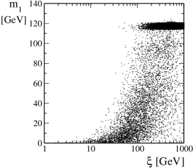
Figure 1: Mass of the lightest Higgs as a function of $\xi$, for a $m_{t}^{\rm pole}=175$ GeV, $M_{\rm SUSY}=350$ GeV and maximal stop mixing. The other parameters are randomly chosen as in Eq. (3.3).

In Fig. 1 we display the mass of the lightest Higgs, $m_{1}$, as a function of the tadpole parameter $\xi$, with the other parameters randomly chosen as in Eq. (3.3). We can see that small values of $\xi$ are associated with a very light mass for the $h_{1}$ state. Such light Higgs states are not excluded by current experimental bounds since their reduced coupling to the SM gauge bosons is small enough to avoid detection.

Before concluding this section, let us comment that regarding the LEP bounds considered, in addition to bounds on the $Zh_{i}h_{j}$ reduced coupling [13], we have also taken into account the LEP limit on the charged Higgs mass [14]. As we will see in the next section, charginos play an important role in the computation of $\varepsilon_{K}$. The tree level chargino mass matrix in the $(\tilde{W},\tilde{H})$ basis reads

$${\cal M}_{\tilde{\chi}^{\pm}}=\left(\begin{array}[]{cc}M_{2}&\sqrt{2}M_{W}\sin\beta e^{-i\theta}\\ \sqrt{2}M_{W}\cos\beta&-\lambda x\end{array}\right)\;,$$ (11)

where $M_{2}$ is the soft wino mass, which was randomly scanned in the interval

$$100\,\mathrm{GeV}<M_{2}<250\,\mathrm{GeV}\,.$$ (12)

We also applied the LEP bound on the chargino and stop masses [28, 29].

4 $\varepsilon_{K}$ in the NMSSM

In the framework of the NMSSM with SCPV, all the SUSY parameters are real. Furthermore the SM does not provide any contribution to any of the CP violation observables, since the CKM matrix is real (and the unitarity trinagle is thus flat). Even so, the physical phases of the Higgs doublets and singlet appear in the scalar fermion, chargino and neutralino mass matrices, as well as in several interaction vertices. In what follows our aim is to investigate whether or not these physical phases can account for the experimental value of $\varepsilon_{K}=(2.284\pm 0.014)\times 10^{-3}$ [30].

4.1 Dominant contributions to $\varepsilon_{K}$

Let us now proceed to compute the contributions to the indirect CP violation parameter of the kaon sector, namely $\varepsilon_{K}$, which is defined as

$$\varepsilon_{K}\simeq\frac{e^{i\pi/4}}{\sqrt{2}}\frac{\operatorname{Im}\mathcal{M}_{12}}{\Delta m_{K}}\;.$$ (13)

In the latter $\Delta m_{K}$ is the long- and short-lived kaon mass difference, and $\mathcal{M}_{12}$ is the off-diagonal element of the neutral kaon mass matrix, related to the effective hamiltonian that governs $\Delta S=2$ transitions as

$$\mathcal{M}_{12}=\frac{\langle K^{0}|\mathcal{H}_{\text{eff}}^{\Delta S=2}|\bar{K}^{0}\rangle}{2m_{K}}\;,\quad\text{with}\qquad\mathcal{H}_{\text{eff}}^{\Delta S=2}=\sum_{i}c_{i}{\mathcal{O}}_{i}\;.$$ (14)

In the above $c_{i}$ are the Wilson coefficients and ${\mathcal{O}}_{i}$ the local operators. In the presence of SUSY contributions, the Wilson coefficients can be decomposed as $c_{i}=c_{i}^{W}+c_{i}^{H^{\pm}}+c_{i}^{\tilde{\chi}^{\pm}}+c_{i}^{\tilde{g}}+c_{i}^{\tilde{\chi}^{0}}$. As discussed in Ref. [21], in the present class of models where there are no contributions from the SM, the chargino mediated box diagrams give the leading supersymmetric contribution, and the $\Delta S=2$ transition is largely dominated by the $(V-A)$ four fermion operator $\mathcal{O}_{1}$. The contributions to $\varepsilon_{K}$ become more transparent if one works in the weak basis for the $\tilde{W}-\tilde{H}$. It can be seen that the leading contribution arises from the box diagrams depicted in Fig. 2.

Figure 2: Box diagrams associated with the leading chargino contribution to $\varepsilon_{K}$.

In the limit of degenerate masses for the left-handed up-squarks, $\operatorname{Im}\mathcal{M}_{12}$ is given by [21]

$$\operatorname{Im}\mathcal{M}_{12} = \frac{2G_{F}^{2}f^{2}_{K}m_{K}m_{W}^{4}}{3\pi^{2}\langle m_{\tilde{q}}\rangle^{8}}(V_{td}^{*}V_{ts})m_{t}^{2}\left|e^{i\theta}\;m_{\tilde{W}}-\cot\beta\;m_{\tilde{H}}\right|$$ (15)

$$\times\left\{\Delta A_{U}\sin[\varphi_{\chi}-\theta]\;{(M^{2}_{\tilde{Q}})}_{12}\;I(r_{\tilde{W}},r_{\tilde{H}},r_{\tilde{u}_{L}},r_{\tilde{t}_{R}})\right\}\;,$$

where $f_{K}$ is the Kaon decay constant and $m_{K}$ the Kaon mass [30]; $V_{ij}$ are the $V_{\mathrm{CKM}}$ elements, whose numerical values ($V_{td}=0.0066$ and $V_{ts}=-0.04$) reflect the fact that we are dealing with a flat unitarity triangle; $\langle m_{\tilde{q}}\rangle$ is the average squark mass, which we take equal to $M_{\rm SUSY}$; $m_{\tilde{W}}=M_{2}$ is the wino mass, $m_{\tilde{H}}=\mu$ is the higgsino mass and $\varphi_{\chi}=\arg(e^{i\theta}m_{{\tilde{W}}}-\cot\beta\;m_{{\tilde{H}}})$. ${(M^{2}_{\tilde{Q}})}_{12}$ parametrises the non-universality in the $LL$ soft breaking masses. The difference $\Delta A_{U}\equiv A_{U}^{13}-A_{U}^{23}$ reflects the non-universality in the soft trilinear terms, which is crucial in order to succeed in complying with the experimental data. Finally, $I$ is the loop function, with $r_{i}=m_{i}^{2}/\langle m_{\tilde{q}}\rangle^{2}$ [21].

4.2 Numerical results and discussion

As shown in [24], a thorough scan of the parameter space confirms that it is indeed possible to satisfy the minimisation conditions of the Higgs potential, have an associated Higgs spectrum compatible with LEP searches and still succeed in generating the observed value of $\varepsilon_{K}$. In the numerical analysis, the free parameters of the model were taken as in Eqs.(3.3,12), with $m_{t}^{\rm pole}=175$ GeV and maximal stop mixing, as in the previously discussed. Moreover, we have taken $100\,\mathrm{GeV}\lesssim M_{2}\lesssim 250$ GeV, and $M_{\rm SUSY}=350$ GeV (a value that reflects the compromise between the need to generate a sufficiently heavy Higgs spectrum and at the same time account for the observed $\varepsilon_{K}$). As noted in [24], saturating the observed value of $\varepsilon_{K}$ favours a regime of low $\tan\beta$, with the maximal values of $\varepsilon_{K}$ being obtained for $\tan\beta\lesssim 3.8$.

In Fig. 3, we plot the maximal value of $\varepsilon_{K}$ in distinct regions of the $(\lambda,\kappa)$ plane. The remaining parameters are chosen so to maximise $\varepsilon_{K}$ and still comply with the experimental bounds. As one can see from this figure, having $\varepsilon_{K}\sim 2\times 10^{-3}$ is associated with values of $\kappa$ and $\lambda$ in the range $[0,0.6]$. In other words, one can easily saturate $\varepsilon_{K}$ in a vast region of the singlet parameter space.

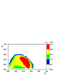
Figure 3: Contours for the maximum value of $\varepsilon_{K}$ in the $\lambda$–$\kappa$ plane for $m_{t}^{\rm pole}=175$ GeV, $M_{\rm SUSY}=350$ GeV, maximal stop mixing and the other parameters as in Eqs. (3.3, 12).

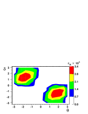
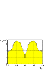
Figure 4: Contours for the maximum value of $\varepsilon_{K}$ in the $\theta$–$\delta$ (left hand-side). Values of $\varepsilon_{K}$ as function of the singlet phase $\varphi_{3}=\delta/3$, depicted by the solid area (right hand-side). All parameters as in Fig. 3.

As expected from the inspection of Eq. (15), there is a strong dependence of $\varepsilon_{K}$ on the phases associated with the Higgs VEVs. In Fig. 4 (left hand-side), we display contour plots for the maximal values of $\varepsilon_{K}$ in the plane generated by the phases $\theta$ and $\delta$. Although, a priori, all the values for the phases $\theta$ and $\delta$ in $[-\pi,\pi]$ are allowed, it is clear from Fig. 4 that the saturation of the experimental value of $\varepsilon_{K}$ can only be achieved for significant values of the singlet and doublet phases. In Fig. 4 (right hand-side) we show the values of $\varepsilon_{K}$ as a function of the singlet phase $\varphi_{3}=\delta/3$. The saturation of the experimental value of $\varepsilon_{K}$ requires the singlet phase to be $|\varphi_{3}|\gtrsim 0.15$.

The consequences of such large CP violating phases are not negligible. Let us recall that $\theta$ and $\delta$ are flavour-conserving phases, and might generate sizable contributions to the electron, neutron and mercury atom EDMs. Although we will not address the EDM problem here, a few remarks are in order: first, let us notice that in the presence of a small singlet coupling $\lambda$, as allowed in our results (see Fig. 3), the EDM constraints on $\delta$ become less stringent [32]. In addition, there are several possible ways to evade the EDM problem, namely reinforcing the non-universality on the trilinear terms (requiring the diagonal terms to be much smaller than the off-diagonal ones or having matrix-factorisable $A$ terms), the existence of cancellations between the several SUSY contributions, and the suppression of the EDMs by a heavy SUSY spectrum [33]. In view of the considerably large parameter space allowed in our results, none of these possibilities should be disregarded.

Finally, and concerning the other CP-violating observables, namely $\varepsilon^{\prime}/\varepsilon$ and the CP asymmetry of the $B_{d}$ meson decay ($a_{J/\psi K_{S}}$), it has been pointed out [20, 34] that this class of models can generate sizable contributions, although saturating the experimental values generally favours a regime of large phases and maximal $LR$ squark mixing.

5 Conclusions

Spontaneous CP violation is a very appealing scenario, strongly motivated by both high- and low-energy arguments. Even though several models have been considered, finding a consistent framework for SCPV is not a trivial task.

The NMSSM with an extra tadpole term in the scalar potential appears to be an excellent candidate for a SCPV scenario. Having a $\mathbb{Z}_{3}$ invariant superpotential preserves the original motivation of the NMSSM to solve the $\mu$ problem of supersymmetry. The tadpole term cures the domain wall problem, and allows the spontaneous breaking of CP. In this model, one can simultaneously saturate $\varepsilon_{K}$ and obtain a sparticle spectrum compatible with current experimental bounds. The analysis of the EDM is certainly critical, and might prove to be a major viability test.

Whether or not CP is explictly or spontaneously broken is a question that must still be aswered. Even though the SM is a most accomplished effective theory, there are strong reasons to believe that it is not the ultimate model of particle physics. It is possible that nature has elected a realisation that includes explicit CP violation, as is the case of the SM. Even so, additional sources of CPV must arise from new physics. As we have tried to argue here, the hypothesis of spontaneous CP violation is extremely appealing. Even though recent studies favour the existence of a non-flat unitarity triangle (thus disfavouring SCPV models), SCPV should not be ruled out. Ultimately, the advent of the LHC and a new generation of colliders will be instrumental in addressing how CP is broken, and which model of particle interactions (SM vs SUSY, minimal or non-minimal) correctly describes nature.

References

- [1] For a review, see G. C. Branco, L. Lavoura and J. P. Silva, “CP Violation”, Int. Series of Monographs on Physics - 113, Oxford Science Publications, 1999.
- [2] G. ’t Hooft et al. (Eds.), Proceedings of the Nato Advanced Summer Institute, Cargèse, 1979, Plenum, New York, 1980.
- [3] T.D. Lee, Phys. Rev. D 8 (1973) 1226; S. Weinberg, Phys. Rev. Lett. 37 (1976) 657.
- [4] S. M. Barr and G. Segrè, Phys. Rev. D 48 (1993) 302; K. S. Babu and S. M. Barr, Phys. Rev. Lett. 72 (1994) 2831.
- [5] A. Strominger and E. Witten, Commun. Math. Phys. 101 (1985) 341; M. Dine, R. G. Leigh and D. A. MacIntire, arXiv:hep-th/9307152.
- [6] S. L. Glashow and S. Weinberg, Phys. Rev. D 15 (1977) 1958; E. A. Paschos, Phys. Rev. D 15 (1977) 1966.
- [7] G. C. Branco, Phys. Rev. D 22 (1980) 2901.
- [8] For a review, see J. F. Gunion, G. L. Kane, H. E. Haber and S. Dawson, “The Higgs Hunter’s Guide”, Addison Wesley, 1990.
- [9] N. Maekawa, Phys. Lett. B 282 (1992) 387.
- [10] H. Georgi and A. Pais, Phys. Rev. D 10 (1974) 1246.
- [11] A. Pomarol, Phys. Lett. B 287 (1992) 331.
- [12] LEP Higgs Working Group, Note 2002/01.
- [13] LEP Higgs Working Group, Note 2001/04.
- [14] LEP Higgs working group, Note 2001/05.
- [15] H.-P. Nilles, M. Srednicki and D. Wyler, Phys. Lett. B 120 (1983) 346; J. Ellis et al., Phys. Rev. D 39 (1989) 844.
- [16] J. E. Kim and H.-P. Nilles, Phys. Lett. B 138 (1984) 150.
- [17] J. C. Romão, Phys. Lett. B 173 (1986) 309.
- [18] K. S. Babu and S. M. Barr, Phys. Rev. D 49 (1994) 2156.
- [19] N. Haba, M. Matsuda and M. Tanimoto, Phys. Rev. D 54 (1996) 6928; S. W. Ham, S. K. Oh and H. S. Song, Phys. Rev. D 61 (2000) 055010.
- [20] A. Pomarol, Phys. Rev. D 47 (1993) 273.
- [21] G. C. Branco, F. Krüger, J. C. Romão and A. M. Teixeira, JHEP 0107 (2001) 027.
- [22] U. Ellwanger, Phys. Lett. B 133 (1983) 187; S. A. Abel, Nucl. Phys. B 480 (1996) 55.
- [23] C. Panagiotakopoulos and K. Tamvakis, Phys. Lett. B 446 (1999) 224, Phys. Lett. B 469 (1999) 145; A. Dedes, C. Hugonie, S. Moretti and K. Tamvakis, Phys. Rev. D 63 (2001) 055009; C. Panagiotakopoulos and A. Pilaftsis, Phys. Rev. D 63 (2001) 055003, Phys. Lett. B 505 (2001) 184.
- [24] C. Hugonie, J. C. Romão and A. M. Teixeira, JHEP 0306 (2003) 020.
- [25] U. Ellwanger, Phys. Lett. B 303 (1993) 271; T. Elliott, S. F. King and P. L. White, PhysL̇ett. B 305 (1993) 71, Phys. Lett B 314 (1993) 56, Phys. Rev. D 49 (1994) 2435.
- [26] M. Carena, H. E. Haber, S. Heinemeyer, W. Hollik, C. E. M. Wagner and G. Weiglein, Nucl. Phys. B 580 (2000) 29; J. R. Espinosa and R.-J. Zhang, Nucl. Phys. B 586 (2000) 3; A. Brignole, G. Degrassi, P. Slavich and F. Zwirner, Nucl. Phys. B 631 (2002) 195.
- [27] U. Ellwanger and C. Hugonie, Eur. Phys. J. C 25 (2002) 297.
- [28] LEP SUSY Working Group, Note 01-03.1.
- [29] LEP SUSY Working Group, Note 02-02.1
- [30] S. Eidelman et al., Phys. Lett. B 592 (2004) 1.
- [31] M. Ciuchini et al., JHEP 9810 (1998) 008.
- [32] M. Matsuda and M. Tanimoto, Phys. Rev. D 52 (1995) 3100.
- [33] S. Khalil, Int. J. Mod. Phys. A 18 (2003) 1697.
- [34] O. Lebedev, Int. J. Mod. Phys. A 15 (2000) 2987.