Supersymmetric approximations to the 3D supersymmetric $O(N)$ model

Abstract

We develop several non-perturbative approximations for studying the dynamics of a supersymmetric $O(N)$ model which preserve supersymmetry. We study the phase structure of the vacuum in both the leading order in large-$N$ approximation as well as in the Hartree approximation, and derive the finite temperature renormalized effective potential. We derive the exact Schwinger-Dyson equations for the superfield Green functions and develop the machinery for going beyond the next to leading order in large-$N$ approximation using a truncation of these equations which can also be derived from a two-particle irreducible effective action.

I Introduction

Theories with supersymmetry (SUSY) have been very attractive to theoretical physicists because they solve the problem of taming the quadratic divergences associated with mass renormalization of scalar fields Wess and Bagger (1992). This cancellation of mass corrections when one includes the related boson and fermion loops is most apparent in the superspace formulation of supersymmetry. If supersymmetry turns out to be a good representation of reality, it would be nice to have approximate analytical methods of understanding the phase structure and dynamics of these theories. Recent advances in approximation schemes to field theory have shown that approximations based on two-particle irreducible (2-PI) effective actions Cornwall et al. (1974); Luttinger and Ward (1960); Baym (1962) have the potential of leading to thermalization of quantum fields Berges and Cox (2001); Aarts and Berges (2001); Berges (2002); Aarts et al. (2002); Cooper et al. (2003a, b). These approximations also allow one to study the dynamics of phase transitions when the appropriate order parameter is found. What we would like to show here is that the methodology used in obtaining the aforementioned approximations in scalar field theories, can easily be generalized to the supersymmetric extension of the theory. In fact, when the superspace formalism is in terms of polynomial interactions of scalar superfields, standard field theory approximations such as large-$N$ expansions Wilson (1973); Cornwall et al. (1974); Coleman et al. (1974), Hartree approximations Schnitzer (1974); Chang (1975); Cooper et al. (1986); Cooper and Mottola (1987); Pi and Samiullah (1987); Boyanovsky et al. (1994) and their resummations via self consistent Schwinger-Dyson equation methods (or effective 2-PI actions) automatically preserve supersymmetry at zero temperature.

The new feature in this work that differentiates it from our previous studies of scalar $\phi^{4}$ field theory Cooper et al. (2003a, b); Blagoev et al. (2001); Mihaila et al. (2001) is that the superfields now depend on anticommuting Grassmann variables as well as the usual space-time coordinates and the action includes integration not only over Minkowski space (here 2+1 dimensional) but also over the two component Majorana spinor $\theta$ of Grassmann coordinates. The superfields contain both bosonic and fermionic degrees of freedom with the interactions dictated by the need for invariance under the supersymmetry transformations.

At finite temperature, supersymmetry is softly broken Das and Kaku (1978). However this occurs in a way which does not affect the cancellation of ultraviolet divergences, since the finite temperature modifications of the super-propagators only affects the infrared physics. Thus the use of supergraphs maintains its usefulness even at finite temperature.

The model we will study is the $O(N)$ supersymmetric $\Phi^{4}$ model, which is actually a scalar $\phi^{6}$ field theory interacting with fermions in a manner consistent with SUSY. This model has recently been studied by Moshe and Zinn-Justin Moshe and Zinn-Justin (2003) (referred to as MZJ in what follows) and by Feinberg, Moshe, and Smolkin Feinberg et al. (2005) in 2+1 dimensions at finite temperature in the leading order in large-$N$ approximation. Their interest was mainly in the spontaneous breakdown of scale invariance but they also found an interesting phase structure which depended on the sign of the renormalized mass parameter as well as the value of the renormalized coupling constant. In this work we will formulate the same model in a slightly more convenient way using the Hubbard-Stratonovich formalism. We will compare the leading order in large-$N$ approximation to the Hartree approximation. We will find that although the two approximations lead to identical dynamics when the expectation value of $\phi$ is zero, the ground states found in these two approximations are quite different and lend themselves to exploring different types of phase transitions. In both approximations the vacuum is degenerate. For some choices of the parameters on finds in both approximations that the states with zero and non zero expectation value of $\phi$ can coexist. This possibility leads to interesting dynamical questions of how an initial state prepared at high temperature and then allowed to expand would choose one or the other vacuum. In this paper we also derive the exact Schwinger-Dyson equations for the superfields in terms of the auxiliary fields with a future goal of doing dynamical simulations as well as studying whether the vacuum degeneracy gets lifted.

In what follows we will use as much as possible the notation of earlier studies of the phase structure of these models which is found in the work of Moshe and Zinn-Justin Moshe and Zinn-Justin (2003) and Shifman, Vainshtein, and Voloshin Shifman et al. (1999). The paper is organized as follows. In section II we discuss the minimal supersymmetric action and derive the large-$N$ and Hartree approximations. We also derive the exact Schwinger-Dyson equations and derive two related approximations that resum the next to leading order large-$N$ approximation. In section three we derive the effective potential for both the leading order large-$N$ and Hartree approximations and discuss the phase structure of the vacuum as well as the behavior of the effective potential at finite temperature. We summarize our results in section IV.

II Minimal supersymmetric action

The minimal action for $N$ commuting superfields in $d$ space-time dimensions for $2\leq d\leq 3$ is given by:

$$\begin{split}S[\Phi]&=\int\mathrm{d}s\>\biggl{\{}\,\frac{1}{2}\,\bigl{[}\bar{D}\,\Phi_{i}(s)\bigr{]}\cdot\bigl{[}D\,\Phi_{i}(s)\bigr{]}\\ &\qquad\qquad\qquad+2N\,\mathcal{W}\bigl{[}\Phi(s)/\sqrt{N}\bigr{]}\,\biggr{\}}\>,\end{split}$$ (1)

where $s=(x^{\mu},\theta_{a})$ with $\mu=0,\dotsc,d-1$ and $a=1,2$ and where we have used a summation convention for the $N$ superfields with $i=1,\dotsc,N$. The integration measure $\mathrm{d}s$ is given by:

$$\mathrm{d}s=\mathrm{d}^{d}x\,\mathrm{d}^{2}\theta=\mathrm{d}^{d}x\,\mathrm{d}\bar{\theta}_{1}\mathrm{d}\theta_{1}/2=i\>\mathrm{d}^{d}x\,\mathrm{d}\theta_{2}\,\mathrm{d}\theta_{1}\>.$$ (2)

The superfields $\Phi_{i}(s)$ can be expanded into commuting and anticommuting components. We write:

$$\Phi_{i}(s)=\phi_{i}(x)+\bar{\theta}\cdot\psi_{i}(x)+\frac{1}{2}\,\bar{\theta}\cdot\theta\,F_{i}(x)\>.$$ (3)

The superfields commute at the same superspace point. Superderivative spinors are defined by:

$$D=+\bar{\partial}-i\,\partial\!\!\!/\cdot\theta\>,\qquad\bar{D}=-\partial+i\,\bar{\theta}\cdot\partial\!\!\!/\>,$$ (4)

where $\partial$ and $\bar{\partial}$ are Grassmann derivatives with respect to $\theta$ and $\bar{\theta}$ respectively. Properties of the superderivatives are further discussed in appendix B.

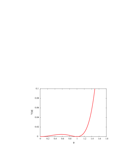
Figure 1: (Color online) Plot of the classical potential for $N=1$ as a function of $\phi$ for the case $\lambda=1$, $\phi_{0}=1$.

For the $O(N)$ model, we choose a superpotential of the form:

$$2N\,\mathcal{W}\bigl{[}\Phi(s)/\sqrt{N}\bigr{]}=\frac{\lambda}{8N}\,\Bigl{[}\,\Phi_{i}^{2}(s)-N\,\phi_{0}^{2}\,\Bigr{]}^{2}\>,$$ (5)

where $\phi_{0}$ is a constant (non-Grassmann). This potential is fourth order in the superfields but sixth order in the scalar fields. In terms of component fields, the action (1) becomes:

$$\!\!S[\phi,\psi,F]=\frac{1}{2}\!\int\!\mathrm{d}^{d}x\,\Bigl{\{}\bigl{[}\partial_{\mu}\phi_{i}(x)\bigr{]}\,\bigl{[}\partial^{\mu}\phi_{i}(x)\bigr{]}+F_{i}^{2}(x)\ \\ +\frac{\lambda}{N}\,X(x)\,\phi_{i}(x)F_{i}(x)\\ +\bar{\psi}_{i}(x)\cdot\bigl{(}\,i\,\delta_{ij}\,\gamma^{\mu}\,\partial_{\mu}-M_{ij}\,\bigr{)}\cdot\psi_{j}(x)\,\Bigr{\}}$$ (6)

where

$$\begin{split}X(x)&=\frac{1}{2}\ \Bigl{[}\,\sum_{j}\phi_{j}^{2}(x)-N\,\phi_{0}^{2}\,\Bigr{]}\>,\\ M_{ij}(x)&=\frac{\lambda}{8N}\,\bigl{[}\,4\,\delta_{ij}\,X(x)+\phi_{i}(x)\,\phi_{j}(x)\,\bigr{]}\>,\end{split}$$ (7)

We see here that $F_{i}(x)$ is not a dynamical variable. Varying the action with respect to $F_{i}(x)$ gives the constraint:

$$F_{i}(x)=-\frac{\lambda}{2N}\,X(x)\,\phi_{i}(x)\>.$$ (8)

Using this result, the action (6) becomes:

$$S[\phi,\psi]=\frac{1}{2}\int\mathrm{d}^{d}x\,\Bigl{\{}\bigl{[}\partial_{\mu}\phi_{i}(x)\bigr{]}\,\bigl{[}\partial^{\mu}\phi_{i}(x)\bigr{]}-2\,V(\phi)\\ +\bar{\psi}_{i}(x)\cdot\bigl{(}\,i\,\delta_{ij}\,\gamma^{\mu}\,\partial_{\mu}-M_{ij}\,\bigr{)}\cdot\psi_{j}(x)\,\Bigr{\}}\>.$$ (9)

where

$$V(\phi)=\frac{\lambda^{2}}{8N^{2}}\,X^{2}(x)\,\bigl{[}\,2\,X(x)+N\,\phi_{0}^{2}\,\bigr{]}\>.$$ (10)

A graph of the classical scalar potential $V(\phi)$ for $N=1$, $\lambda=1$, and $\phi_{0}=1$, as a function of $\phi$ is shown in Fig. 1. The curve is symmetric about the origin, with two minima’s at $\phi=0$ and $\phi=\phi_{0}$.

II.1 Large-$N$ approximation

For the large-$N$ approximation, it is easier to count powers of $1/N$ by introducing a commuting composite superfield $\chi(s)$. In general, this can be done for an arbitrary polynomial Lagrangian by introducing a functional delta function of the type:

$$\int\mathrm{d}\chi\,\delta\Bigl{[}\,\chi(x)-\frac{\lambda}{2N}\,\phi_{i}^{2}(x)\,\Bigr{]}=1\>,$$ (11)

into the path integral. This is the strategy used by MZJ. However, for quartic scalar interactions, it is simpler to use the Hubbard-Stratonovich transformation to convert the quartic term into a Gaussian at the cost of an additional integration, using the identity:

$$\int\mathrm{d}\phi\,\exp\bigl{(}\,-\tfrac{1}{2}\,\phi\,G^{-1}\,\phi+j\,\phi\,\bigr{)}\\ =\exp\bigl{\{}\,\tfrac{1}{2}\,j\,G\,j-\tfrac{1}{2}\,\mathrm{Tr}[\,\ln\,G^{-1}\,]\,\bigr{\}}\>,$$ (12)

with $j$ being proportional to $\phi_{i}^{2}(x)$. The same trick applies to the superfield case. This is equivalent to introducing a commuting composite super field $\chi(s)$ by subtracting from the action (1) a term of the form:

$$\int\mathrm{d}s\>\frac{N}{2\lambda}\,\biggl{\{}\chi(s)\ {\color[rgb]{0,0,0}-}\ \frac{\lambda}{2N}\,\Bigl{[}\,\sum_{j=1}^{N}\Phi_{j}^{2}(s)-N\,\phi_{0}^{2}\,\Bigr{]}\biggr{\}}^{2}\>.$$ (13)

This leads to an equivalent action given by:

$$S[\Phi,\chi;J,K]=$$ (14)

$$\int\mathrm{d}s\,\biggl{\{}\,\frac{1}{2}\,\Bigl{[}\,(\bar{D}\,\Phi_{i}(s))\cdot(D\,\Phi_{i}(s))\ {\color[rgb]{0,0,0}+}\ \chi(s)\,\Phi_{i}^{2}(s)\,\Bigr{]}$$

$$-\frac{N}{\lambda}\Bigl{[}\frac{\chi^{2}(s)}{2}{\color[rgb]{0,0,0}-}{\color[rgb]{0,0,0}2\mu}\,\chi(s)\Bigr{]}+J_{i}(s)\Phi_{i}(s)+K(s)\chi(s)\biggr{\}}\>,$$

where ${\color[rgb]{0,0,0}2\mu=-\lambda\,\phi_{0}^{2}/2}$ ($\mu$ has units of mass). One of the things we will show is that the action (14) reproduces the results of MZJ and leads to a simpler formula for the corrections to large-$N$. The supergenerating functional $Z[J,K]$ is defined by the path integral:

$$Z[J,K] =\exp\bigl{\{}iW[J,K]\,\bigr{\}}$$ (15)

$$=\int\mathrm{d}\chi\prod_{i}\int\mathrm{d}\Phi_{i}\>\exp\bigl{\{}\,iS[\Phi,\chi;J,K]\,\bigr{\}}\>.$$

Average values of the superfields are obtained by differentiation of the supergenerating functional:

$$\begin{split}\langle\,\Phi_{i}(s)\,\rangle=\frac{1}{iZ}\,\frac{\partial Z[J,K]}{\partial J_{i}(s)}=\frac{\partial W[J,K]}{\partial J_{i}(s)}\>,\\ \langle\,\chi(s)\,\rangle=\frac{1}{iZ}\,\frac{\partial Z[J,K]}{\partial K(s)}=\frac{\partial W[J,K]}{\partial K(s)}\>.\end{split}$$ (16)

We introduce an inverse Green function $G^{-1}_{ij}[\chi](s,s)$ by:

$$G^{-1}_{ij}[\chi](s,s^{\prime})=\bigl{[}\,\bar{D}\cdot D\ {\color[rgb]{0,0,0}-}\ \chi(s)\,\bigr{]}\,\delta_{ij}\,\delta(s,s^{\prime})\>,$$ (17)

so that the Green function $G_{ij}[\chi](s,s^{\prime})$ satisfies the superdifferential equation:

$$\bigl{[}\,\bar{D}\cdot D\ {\color[rgb]{0,0,0}-}\ \chi(s)\,\bigr{]}\,G_{ij}(s,s^{\prime})=\delta_{ij}\,\delta(s,s^{\prime})\>.$$ (18)

Integrating by parts, the action (14) can be written as:

$$S[\Phi,\chi; J,K]\!=\!-\frac{1}{2}\int\!\!\mathrm{d}s\!\!\int\!\mathrm{d}s^{\prime}\,\Phi_{i}(s)G^{-1}_{ij}[\chi](s,s^{\prime})\Phi_{j}(s^{\prime})$$

$$-\int\mathrm{d}s\,\biggl{\{}\,\frac{N}{\lambda}\,\Bigl{[}\,\frac{\chi^{2}(x,\theta)}{2}\ {\color[rgb]{0,0,0}-}\ {\color[rgb]{0,0,0}2\mu}\,\chi(x,\theta)\,\Bigr{]}$$

$$+J_{i}(s)\,\Phi_{i}(s)+K(s)\,\chi(s)\,\biggr{\}}\>.$$ (19)

The action (II.1) is quadratic in the fields $\Phi_{i}(s)$ so we can integrate them out of the generating functional. This gives:

$$Z[J,K]=\mathcal{N}\int\mathrm{d}\chi\,\exp\bigl{\{}\,iS^{\prime}[\chi;J,K]\,\bigr{\}}\>,$$ (20)

where $\mathcal{N}$ is a constant and:

$$S^{\prime}[\chi;J,K]=\int\mathrm{d}s\biggl{\{}\,-\frac{N}{\lambda}\,\Bigl{[}\,\frac{\chi^{2}(s)}{2}\ {\color[rgb]{0,0,0}-}\ {\color[rgb]{0,0,0}2\mu}\,\chi(s)\,\Bigr{]}\\ +K(s)\,\chi(s)+\frac{iN}{2}\,\ln\{G^{-1}_{ii}[\chi](s,s)\}\biggr{\}}\\ +\frac{1}{2}\int\mathrm{d}s\int\mathrm{d}s^{\prime}\,J_{i}(s)\,G_{ij}[\chi](s,s^{\prime})\,J_{j}(s)\>.$$ (21)

The integral over $\chi(s)$ in (20) is now done by the method of steepest descent. We expand the exponent about a superfield $\chi_{0}$:

$$S^{\prime}[\chi;J,K]=S^{\prime}[\chi_{0};J,K]\\ +\int\mathrm{d}s\,\bigl{[}\,\chi(s)-\chi_{0}(s)\,\bigr{]}\,\Bigl{[}\,\frac{\partial S^{\prime}[\chi;J,K]}{\partial\chi(s)}\,\Bigr{]}_{\chi_{0}}\\ +\frac{1}{2}\int\mathrm{d}s\int\mathrm{d}s^{\prime}\,\bigl{[}\,\chi(s)-\chi_{0}(s)\,\bigr{]}\,\bigl{[}\,\chi(s^{\prime})-\chi_{0}(s^{\prime})\,\bigr{]}\,\\ \times\Bigl{[}\,\frac{\partial^{2}S^{\prime}[\chi;J,K]}{\partial\chi(s)\,\partial\chi(s^{\prime})}\,\Bigr{]}_{\chi_{0}}+\dotsb$$ (22)

where we choose $\chi_{0}$ such that the linear term vanishes. This gives the stationary condition:

$$\chi_{0}(s)=2\mu\ {\color[rgb]{0,0,0}+}\ \frac{\lambda}{2}\Bigl{[}\,\frac{1}{N}\,\Phi_{i}^{2}[\chi_{0},J](s)+G_{ii}[\chi_{0}](s,s)/i\,\Bigr{]}\\ +\frac{\lambda}{N}\,K(s)\>.$$ (23)

Evaluated at $K(s)=0$, Eq. (23) is the supergap equation. Here we have defined $\Phi_{i}[\chi_{0},J](s)$, which is a functional of $\chi_{0}$ and $J$, as the solution of the integral equation:

$$\Phi_{i}[\chi_{0},J](s)=\int\mathrm{d}s^{\prime}\,G_{ij}[\chi_{0}](s,s^{\prime})\,J_{j}(s^{\prime})\>.$$ (24)

We have the remaining action, which is given by:

$$W[J,K]=W_{0}[J,K]+\frac{i}{2}\,\int\mathrm{d}s\,\ln\{D^{-1}(s,s)\}+\dotsb$$ (25)

where

$$W_{0}[J,K]=\int\mathrm{d}s\biggl{\{}\,-\frac{N}{\lambda}\,\Bigl{[}\,\frac{\chi_{0}^{2}(s)}{2}\ {\color[rgb]{0,0,0}-}\ {\color[rgb]{0,0,0}2\mu}\,\chi_{0}(s)\,\Bigr{]}\\ +K(s)\,\chi_{0}(s)+\frac{iN}{2}\,\ln\bigl{[}G^{-1}_{ii}[\chi_{0}](s,s)\bigr{]}\biggr{\}}\\ +\frac{1}{2}\int\mathrm{d}s\int\mathrm{d}s^{\prime}\,J_{i}(s)\,G_{ij}[\chi_{0}](s,s^{\prime})\,J_{j}(s)\>,$$ (26)

and where

$$\begin{split}D^{-1}(s,s^{\prime})&=\frac{1}{N}\Bigl{[}\,\frac{\partial^{2}S^{\prime}[\chi;J,K]}{\partial\chi(s)\,\partial\chi(s^{\prime})}\,\Bigr{]}_{\chi_{0}}\\ &=D^{-1}_{0}(s,s^{\prime})+\Pi_{0}(s,s^{\prime})\>,\end{split}$$ (27)

with:

$$D^{-1}_{0}(s,s^{\prime})=-\frac{1}{\lambda}\,\delta(s,s^{\prime})\>,$$ (28)

and

$$\Pi_{0}(s,s^{\prime})\\ =\frac{1}{N}\,\Phi_{i}[\chi_{0}](s)\,G_{ij}[\chi_{0}](s,s^{\prime})\,\Phi_{j}[\chi_{0}](s^{\prime})\\ +\frac{1}{2i}\,G_{ij}[\chi_{0}](s,s^{\prime})\,G_{ji}[\chi_{0}](s^{\prime},s)\>.$$ (29)

The vertex function is given by a Legendre transformation:

$$\Gamma[\Phi,\chi]=W[J,K]\\ -\int\mathrm{d}s\,\Bigl{\{}\,J_{i}(s)\,\Phi_{i}(s)+K(s)\,\chi(s)\,\Bigr{\}}\>,$$ (30)

where

$$\begin{split}\Phi_{i}(s)&=\frac{\partial W[J,K]}{\partial J_{i}(s)}=\Phi_{i}[\chi_{0}](s)+\frac{1}{N}\Phi_{1\,i}(s)+\cdots\\ \chi(s)&=\frac{\partial W[J,K]}{\partial K(s)}=\chi_{0}(s)+\frac{1}{N}\chi_{1}(s)+\cdots\end{split}$$ (31)

So, to first order in $1/N$, we find the effective action:

$$\Gamma[\Phi,\chi]=-\frac{1}{2}\int\!\mathrm{d}s\int\!\mathrm{d}s^{\prime}\,\Bigl{\{}\Phi_{i}(s)G^{-1}_{ij}[\chi](s,s^{\prime})\Phi_{j}(s^{\prime})\Bigr{\}}$$

$$-\int\mathrm{d}s\>\Bigl{\{}\,\frac{N}{\lambda}\,\Bigl{[}\,\frac{\chi^{2}(s)}{2}\ {\color[rgb]{0,0,0}-}\ {\color[rgb]{0,0,0}2\mu}\,\chi(s)\,\Bigr{]}$$ (32)

$$\qquad+\frac{iN}{2}\,\ln\bigl{[}G^{-1}_{ii}[\chi](s,s)\bigr{]}+\frac{i}{2}\,\ln\bigl{[}D^{-1}[\chi](s,s)\bigr{]}\Bigr{\}}\>,$$

which is the classical action plus the trace-log terms.

We list again here the superequations to be solved in first order large-$N$. We set the currents to zero, and arrive at the following equations:

$$\bigl{[}\,\bar{D}\cdot D\ {\color[rgb]{0,0,0}-}\ \chi(s)\,\bigr{]}\,\Phi_{i}(s)=0\>,$$ (33a)

$$\bigl{[}\,\bar{D}\cdot D\ {\color[rgb]{0,0,0}-}\ \chi(s)\,\bigr{]}\,G_{ij}(s,s^{\prime})=\delta_{ij}\,\delta(s,s^{\prime})\>,$$ (33b)

$$\chi(s)=2\mu\ {\color[rgb]{0,0,0}+}\ \frac{\lambda}{2}\,\Bigl{[}\,\Phi_{i}^{2}(s)/N+G_{ii}(s,s)/i\,\Bigr{]}\>.$$ (33c)

From Eq. (II.1), for $N=1$, the effective large-N superpotential is given by:

$$V_{\text{N}}[\Phi,\chi]=\int\mathrm{d}^{2}\theta\,\Bigl{\{}\,-\frac{1}{2}\,(\bar{\theta}\cdot\theta)\,F^{2}{\color[rgb]{0,0,0}-}\ \frac{1}{2}\,\chi\,\Phi^{2}\\ {\color[rgb]{0,0,0}+}\frac{1}{\lambda}\,\Bigl{[}\,\frac{\chi^{2}}{2}\ {\color[rgb]{0,0,0}-}\ {\color[rgb]{0,0,0}2\mu}\,\chi\,\Bigr{]}-\frac{i}{2}\,\mathrm{Tr}[\,\ln\,G^{-1}[\Phi,\chi]\,]\,\Bigr{\}}\>,$$ (34)

where the first term comes from the kinetic part of the energy.

II.2 Hartree equations

In this section, we develop the Hartree equations for this system. We start with the action given in Eq. (1):

$$\begin{split}S[\Phi]&=\int\mathrm{d}s\>\biggl{\{}\,\frac{1}{2}\,\bigl{[}\bar{D}\,\Phi_{i}(s)\bigr{]}\cdot\bigl{[}D\,\Phi_{i}(s)\bigr{]}\\ &\qquad\qquad\qquad+\frac{\lambda}{8N}\,\bigl{[}\,\Phi_{j}^{2}(s)-N\,\phi_{0}^{2}\,\bigr{]}^{2}\,\biggr{\}}\>.\end{split}$$ (35)

The equations of motion are given by:

$$\bigl{(}\,\bar{D}D{\color[rgb]{0,0,0}-}{\color[rgb]{0,0,0}2\mu}\,\bigr{)}\,\Phi_{i}(s){\color[rgb]{0,0,0}-}\frac{\lambda}{2N}\,\Phi_{j}^{2}(s)\,\Phi_{i}(s)=J_{i}(s)\>,$$ (36)

where $J_{i}(s)$ is an external supercurrent, and where we have again set ${\color[rgb]{0,0,0}2\mu=-\lambda\phi_{0}^{2}/2}$. Considering this as an operator equation and taking expectation values gives the classical equation:

$$\bigl{(}\bar{D}D{\color[rgb]{0,0,0}-}2\mu\bigr{)}\langle\,\Phi_{i}(s)\,\rangle{\color[rgb]{0,0,0}-}\frac{\lambda}{2N}\langle\,\Phi_{j}^{2}(s)\Phi_{i}(s)\,\rangle\!=\!J_{i}(s)\>.$$ (37)

The Hartree approximation sets the third order connected Green function to zero:

$$\frac{\partial G_{ij}(s,s^{\prime})}{\partial J_{k}(s^{\prime\prime})}=0\>.$$ (38)

So this means that the third order correlator is:

$$\langle\,\Phi_{j}^{2}(s)\,\Phi_{i}(s)\,\rangle=\bigl{[}\,\langle\,\Phi_{j}(s)\,\rangle^{2}+G_{jj}(s,s)/i\,\bigr{]}\,\langle\,\Phi_{i}(s)\,\rangle\\ +2\,G_{ij}(s,s)\,\langle\,\Phi_{j}(s)\,\rangle/i\>.$$ (39)

So the equations of motion become:

$$\Bigl{\{}\bigl{[}\,\bar{D}D{\color[rgb]{0,0,0}-}\frac{\lambda}{2N}\,[\,\langle\,\Phi_{k}(s)\,\rangle^{2}+G_{kk}(s,s)/i\,]{\color[rgb]{0,0,0}-}2\mu\,\bigr{]}\,\delta_{ij}\\ {\color[rgb]{0,0,0}-}\frac{\lambda}{N}\,G_{ij}(s,s)/i\,\Bigr{\}}\,\langle\,\Phi_{j}(s)\,\rangle=0\>,$$ (40)

and

$$\Bigl{\{}\bigl{[}\,\bar{D}D{\color[rgb]{0,0,0}-}\frac{\lambda}{2N}\,[\,\langle\,\Phi_{l}(s)\,\rangle^{2}+G_{ll}(s,s)/i\,]{\color[rgb]{0,0,0}-}2\mu\,\bigr{]}\,\delta_{ij}\\ {\color[rgb]{0,0,0}-}\frac{\lambda}{N}\,\Phi_{i}(s)\Phi_{j}(s)\,\Bigr{\}}\,G_{jk}(s^{\prime},s^{\prime\prime})\\ {\color[rgb]{0,0,0}-}\frac{\lambda}{N}\,G_{ij}(s,s)\,G_{jk}(s,s^{\prime})/i=\delta_{ik}\delta(s,s^{\prime})\>.$$ (41)

For $N=1$, these equations reduce to:

$$\Bigl{\{}\,\bar{D}D{\color[rgb]{0,0,0}-}\frac{\lambda}{2}\,[\,\Phi^{2}(s)+3\,G(s,s)/i\,]{\color[rgb]{0,0,0}-}2\mu\,\Bigr{\}}\,\Phi(s)=0\>,$$ (42)

and

$$\Bigl{\{}\,\bar{D}D{\color[rgb]{0,0,0}-}\frac{3\lambda}{2}\,[\,\Phi^{2}(s)+G(s,s)/i\,]{\color[rgb]{0,0,0}-}2\mu\,\Bigr{\}}\,G(s,s^{\prime})\\ =\delta(s,s^{\prime})\>.$$ (43)

We now notice that these equations of motion are generated from an action, given by:

$$S_{H}[\Phi,\chi]=-\int\mathrm{d}s\,\Bigl{\{}\,\frac{1}{2}\,\Phi(s)\,\bigl{[}\,\bar{D}D\ {\color[rgb]{0,0,0}-}\ \chi(s)\,\bigr{]}\,\Phi(s)\\ +\frac{\lambda}{4}\,\Phi^{4}(s)-\frac{1}{3\lambda}\,\bigl{[}\,\chi^{2}(s)/2\ {\color[rgb]{0,0,0}-}\ {\color[rgb]{0,0,0}2\mu}\,\chi(s)\,\bigr{]}\\ +\frac{i}{2}\,\mathrm{Tr}\{\ln[\,\bar{D}D\ {\color[rgb]{0,0,0}-}\ \chi(s)\,]\}\Bigr{\}}$$ (44)

where $\chi(s)$ is an auxiliary superfield. The equations of motion generated from this action is given by:

$$[\,\bar{D}D\ {\color[rgb]{0,0,0}-}\ \chi(s)-\lambda\Phi^{2}(s)\,]\,\Phi(s)=0\>,$$ (45a)

$$[\,\bar{D}D\ {\color[rgb]{0,0,0}-}\ \chi(s)\,]\,G(s,s^{\prime})=\delta(s,s^{\prime})\>,$$ (45b)

$$\chi(s)=2\mu\ {\color[rgb]{0,0,0}+}\ (3\lambda/2)\,[\,\Phi^{2}(s)+G(s,s)/i\,]\>,$$ (45c)

and agrees with Eqs. (42) and (43). The effective Hartree superpotential is then given by:

$$V_{\text{H}}[\Phi,\chi]=\int\mathrm{d}^{2}\theta\,\Bigl{\{}\,-\frac{1}{2}\,(\bar{\theta}\cdot\theta)\,F^{2}\ {\color[rgb]{0,0,0}-}\ \frac{1}{2}\,\chi\,\Phi^{2}-\frac{\lambda}{4}\,\Phi^{4}\\ {\color[rgb]{0,0,0}+}\frac{1}{3\lambda}\,\Bigl{[}\,\frac{\chi^{2}}{2}\ {\color[rgb]{0,0,0}-}\ {\color[rgb]{0,0,0}2\mu}\,\chi\,\Bigr{]}-\frac{i}{2}\,\mathrm{Tr}[\,\ln G^{-1}[\Phi,\chi]\,]\,\Bigr{\}}\>,$$ (46)

II.3 Schwinger-Dyson equations and the 2-PI effective action

We develop in this section the coupled supersymmetric Schwinger-Dyson equations for the $O(N)$ model. We first rewrite Eq. (II.1) in an extended field scheme:

$$\!\!S[\Phi,J]=\int\mathrm{d}s\,\Bigl{\{}-\frac{1}{2}\,\int\mathrm{d}s^{\prime}\,\Phi_{a}(s)\,\Delta_{ab}^{-1}(s,s^{\prime})\,\Phi_{b}(s^{\prime})\\ -\frac{1}{6}\,\gamma_{abc}\,\Phi_{a}(s)\,\Phi_{b}(s)\,\Phi_{c}(s)+J_{a}(s)\,\Phi_{a}(s)\,\Bigr{\}}\>.$$ (47)

In the rest of this section, we have suppressed the supercoordinates. In this extended scheme, $a=(0,i)$, with $i=1,2,\dotsc,N$, and we define the extended vectors:

$$\begin{split}\Phi_{a}&=\bigl{(}\,\chi,\Phi_{1},\Phi_{2},\dotsc,\Phi_{N}\,\bigr{)}\>,\\ J_{a}&=\bigl{(}\,J_{0},J_{1},J_{2},\dotsc,J_{N}\,\bigr{)}\>,\end{split}$$ (48)

where $J_{0}=K+N\,\mu/\lambda$, and

$$\Delta_{ab}^{-1}=\begin{pmatrix}D^{-1}&0\\ 0&G^{-1}_{ij}\end{pmatrix}\>,$$ (49)

where $D^{-1}=-N/\lambda$ and $G^{-1}_{ij}=\bar{D}\cdot D\,\delta_{ij}$. The introduction of a composite field $\chi$ enables us to use a cubic supersymmetric interaction rather than the usual quartic term, at the expense of an additional dimension for the superfield vector $\Phi_{a}$. For our case, $\gamma_{abc}$ is fully symmetric, and given by:

$$\gamma_{0ij}=\gamma_{i0j}=\gamma_{ij0}=\delta_{ij}\>,$$ (50)

with all other values zero. The equation of motion for the quantum operators $\hat{\Phi}_{a}$ is given by:

$$\Delta_{ab}^{-1}\,\hat{\Phi}_{b}+\frac{1}{2}\,\gamma_{abc}\,\hat{\Phi}_{b}\,\hat{\Phi}_{c}=J_{a}\>.$$ (51)

The supergenerating functional is given by the path integral (20), which we write as:

$$Z[J]=e^{iW[J]}=\int\mathrm{d}\Phi\,e^{iS[\Phi,J]}\>.$$ (52)

Expectation values of the closed-time-path ordered product of $n$ field operators are given by:

$$\langle\,\mathcal{T}\{\,\hat{\Phi}_{a}\hat{\Phi}_{b}\dotsc\,\}\,\rangle=\frac{1}{i^{n}Z}\,\frac{\partial^{n}Z[J]}{\partial J_{a}\,\partial J_{b}\cdots}\>.$$ (53)

The $n$-point connected supergreen functions are defined by:

$$G_{ab\dotsc}[J]=\frac{\partial^{n}W[J]}{\partial J_{a}\,\partial J_{b}\cdots}\>.$$ (54)

Here $G_{ab\dotsc}[J]$ is fully symmetric with respect to interchange of arguments. In particular for $n=1$:

$$\Phi_{a}[J]\equiv G_{a}[J]=\frac{\partial W[J]}{\partial J_{a}}\>,$$ (55)

which is the average value of the field when evaluated at $J=0$. The vertex function $\Gamma[\Phi]$ is defined by the Legendre transformation:

$$\Gamma[\Phi]=W[J]-J_{a}\,\Phi_{a}\>.$$ (56)

In analogy to the supergreen functions, the $n$-point connected supervertex functions are then defined by:

$$\Gamma_{ab\dotsc}[\Phi]=-\frac{\partial^{n}\Gamma[\Phi]}{\partial\Phi_{a}\,\partial\Phi_{b}\cdots}\>.$$ (57)

In particular for $n=1$:

$$J_{a}[\Phi]\equiv-\Gamma_{a}[\Phi]=-\frac{\partial\Gamma[\Phi]}{\partial\Phi_{a}}\>.$$ (58)

The two-point supergreen functional is the inverse of the two-point supervertex functional. Using the chain rule, we find:

$$\begin{split}G_{ab}[J]\,\Gamma_{bc}[\Phi]&=-\frac{\partial^{2}W[J]}{\partial J_{a}\,\partial J_{b}}\,\frac{\partial^{2}\Gamma[\Phi]}{\partial\Phi_{b}\,\partial\Phi_{c}}\\ &=\frac{\partial\Phi_{b}[J]}{\partial J_{a}}\frac{\partial J_{c}}{\partial\Phi_{b}}=\delta_{ac}\>.\end{split}$$ (59)

Differentiating (59) with respect to $\Phi_{d}$ gives:

$$\frac{\partial G_{ab}[J]}{\partial\Phi_{d}}\,\Gamma_{bc}[\Phi]+G_{ab}[J]\,\Gamma_{dbc}[\Phi]=0\>.$$

Using (59) gives:

$$\frac{\partial G_{ae}[J]}{\partial\Phi_{d}}=-G_{ab}[J]\,\Gamma_{dbc}[\Phi]\,G_{ce}[J]\>.$$ (60)

The Schwinger-Dyson hierarchy of coupled equations is generated by taking the expectation value of the closed-time-path ordered product of Eq. (51). We find:

$$\Delta_{ab}^{-1}\Phi_{b}+\frac{1}{2}\,\gamma_{abc}\,\bigl{(}\,\Phi_{b}\,\Phi_{c}+G_{bc}[J]/i\,\bigr{)}\\ =J_{a}[\Phi]=-\Gamma_{a}[\Phi]=-\frac{\partial\Gamma[\Phi]}{\partial\Phi_{a}}\>.$$ (61)

When evaluated at $J=0$, Eq. (61) is the equation of motion for the fields $\Phi_{a}$. Differentiation of Eq. (61) with respect to $\Phi_{b}$ gives:

$$\Gamma_{ab}[\Phi]=-\frac{\partial^{2}\Gamma[\Phi]}{\partial\Phi_{a}\,\partial\Phi_{b}}=\bar{\Delta}_{ab}^{-1}[\Phi]+\bar{\Sigma}_{ab}[\Phi]\>,$$ (62)

where, from (60):

$$\bar{\Delta}_{ab}^{-1}[\Phi] =\Delta_{ab}^{-1}+\gamma_{abc}\Phi_{c}\>,$$ (63)

$$\bar{\Sigma}_{ab}[\Phi] =\frac{i}{2}\,\gamma_{aa^{\prime}b^{\prime}}\,G_{a^{\prime}a^{\prime\prime}}[J]\,G_{b^{\prime}b^{\prime\prime}}[J]\,\Gamma_{a^{\prime\prime}b^{\prime\prime}b}[\Phi]\>.$$

The three-point supervertex function can now be computed by differentiating (62). We find:

$$\Gamma_{abc}[\Phi]=-\frac{\partial^{2}\Gamma[\Phi]}{\partial\Phi_{a}\,\partial\Phi_{b}\,\partial\Phi_{c}}=\gamma_{abc}+\frac{\partial\bar{\Sigma}_{ab}[\Phi]}{\partial\Phi_{c}}\>.$$ (64)

The bare vertex approximation (BVA) keeps only the first term in this equation, in which case, we find for the self-energy:

$$\bar{\Sigma}_{ab}^{\text{BVA}}[\Phi]=\frac{i}{2}\,\gamma_{aa^{\prime}b^{\prime}}\,G_{a^{\prime}a^{\prime\prime}}[J]\,G_{b^{\prime}b^{\prime\prime}}[J]\,\gamma_{a^{\prime\prime}b^{\prime\prime}b}\>.$$ (65)

Using this approximation to the full self-energy, we invert Eq. (62) by multiplying by $\bar{\Delta}_{aa^{\prime}}[\Phi]\,G_{bb^{\prime}}[J]$ to give the integral equation:

$$G_{ab}[J]=\bar{\Delta}_{ab}[\Phi]-\bar{\Delta}_{aa^{\prime}}[\Phi]\,\bar{\Sigma}_{a^{\prime}b^{\prime}}^{\text{BVA}}[\Phi]\,G_{b^{\prime}b}[J]\>,$$ (66)

which is to be solved self-consistently for $G_{ab}[J]$. The hierarchy of coupled green function equations have now been truncated. The BVA approximation is a conserving approximation in that an action can be constructed, using the methods of Cornwall, Jackiw, and Tomboulis Cornwall et al. (1974), which reproduces these coupled equations. This action is given by:

$$S[\Phi,G]=S_{\text{class}}[\Phi]+\frac{i}{2}\,\mathrm{Tr}\{\ln[\bar{\Delta}^{-1}]\}\\ +\frac{i}{2}\,\mathrm{Tr}\{\ln[\bar{\Delta}^{-1}[\Phi]\,G-1]\}+\Gamma_{2}[G]\>,$$ (67)

where, in the BVA,

$$\Gamma_{2}[G]=-\frac{1}{12}\,\gamma_{abc}\,G_{aa^{\prime}}\,G_{bb^{\prime}}\,G_{cc^{\prime}}\,\gamma_{a^{\prime}b^{\prime}c^{\prime}}\>.$$ (68)

Varying this action with respect to $\Phi$ and $G$ independently, leads to the BVA equations. The natural 2-PI expansion would consist of taking higher and higher loops in $\Gamma_{2}$ (the lowest being two loops). However if one wants to further keep only terms in $\Gamma_{2}$ to a particular order in $1/N$ then one needs to realize that the $\chi$ and $\phi$ pieces of $G$ have different $N$ dependence as seen in Eqs. (48) and (49). This is discussed in detail in Ref. Aarts et al. (2002)

III Effective potential

In this section, we derive effective potentials for the large-$N$ and Hartree approximations in the vacuum at $T=0$ and for finite temperature.

We consider here the spatially homogeneous case where the average superfields depend only on time, and require the average Fermi field to vanish. Thus we write:

$$\Phi_{i}(t,\theta) =\phi_{i}(t)+\frac{1}{2}\,\bar{\theta}\cdot\theta\,F_{i}(t)\>,$$ (69)

$$\chi(t,\theta) =2\,\rho(t)\ {\color[rgb]{0,0,0}-}\ \bar{\theta}\cdot\theta\,R(t)\>.$$ (70)

III.1 Supergreen function

The two-point supergreen function $G(s,s^{\prime})$ is of the form:

$$G_{ij}(s,s^{\prime})=g_{0\,ij}(x,x^{\prime})+\frac{1}{2}\,(\,\bar{\theta}\cdot\theta+\bar{\theta}^{\prime}\cdot\theta^{\prime}\,)\,g_{1\,ij}(x,x^{\prime})\\ {\color[rgb]{0,0,0}-}\bar{\theta}\cdot g_{2\,ij}(x,x^{\prime})\cdot\theta^{\prime}+\frac{1}{4}\,(\bar{\theta}\cdot\theta)\,(\bar{\theta}^{\prime}\cdot\theta^{\prime})\,g_{3\,ij}(x,x^{\prime})\>.$$ (71)

The generalized Ward-Takahashi identity states that:

$$(\,Q+Q^{\prime}\,)\,G_{ij}(s,s^{\prime})=0\>.$$ (72)

Here $Q$ and $Q^{\prime}$ are the supercharge operators, given by:

$$Q=-\bar{\partial}-i\,\partial\kern-5.50003pt/\cdot\theta\>,\qquad Q^{\prime}=-\partial^{\prime}-i\,\partial\kern-5.50003pt/^{\prime}\cdot\theta^{\prime}\>.$$ (73)

Eq. (72) requires that:

$$g_{2\,ij}(x^{\prime},x) =-g_{1\,ij}(x,x^{\prime})-i\,\partial\kern-5.50003pt/g_{0\,ij}(x,x^{\prime})\>,$$ (74a)

$$g_{2\,ij}(x,x^{\prime}) =-g_{1\,ij}(x,x^{\prime})-i\,\partial\kern-5.50003pt/^{\prime}g_{0\,ij}(x,x^{\prime})\>,$$ (74b)

$$g_{3\,ij}(x,x^{\prime}) =-i\,\partial\kern-5.50003pt/g_{1\,ij}(x,x^{\prime})+i\,\partial\kern-5.50003pt/^{\prime}g_{2\,ij}(x^{\prime},x)\>,$$ (74c)

$$g_{3\,ij}(x,x^{\prime}) =-i\,\partial\kern-5.50003pt/^{\prime}g_{1\,ij}(x,x^{\prime})+i\,\partial\kern-5.50003pt/g_{2\,ij}(x,x^{\prime})\>,$$ (74d)

from which we obtain:

$$g_{3\,ij}(x,x^{\prime})=\partial^{\mu}\partial^{\prime}_{\mu}\,g_{0\,ij}(x,x^{\prime})\>,$$ (75)

and

$$\frac{1}{2}\,\bigl{\{}\,\bar{\theta}\cdot g_{2\,ij}(x,x^{\prime})\cdot\theta^{\prime}+\bar{\theta}^{\prime}\cdot g_{2\,ij}(x^{\prime},x)\cdot\theta\,\bigr{\}}\\ =-(\bar{\theta}\cdot\theta^{\prime})\,g_{1\,ij}(x,x^{\prime})+\bar{\theta}\cdot\frac{i}{2}\,\bigl{[}\,\partial\kern-5.50003pt/-\partial\kern-5.50003pt/^{\prime}\,\bigr{]}\cdot\theta^{\prime}\,g_{0\,ij}(x,x^{\prime})\>.$$ (76)

So using (75) and (76), if $G(s,s^{\prime})$ satisfies the Ward-Takahashi identity, it must be of the general form:

$$G(s,s^{\prime})= \Bigl{\{}1+\frac{i}{2}\bar{\theta}\cdot\bigl{[}\partial\!\!\!/-\partial\!\!\!/^{\prime}\bigr{]}\cdot\theta^{\prime}$$ (77)

$$\quad+\frac{1}{4}(\bar{\theta}\cdot\theta)\cdot(\bar{\theta}^{\prime}\cdot\theta^{\prime})\partial^{\mu}\partial^{\prime}_{\mu}\Bigr{\}}\,g_{0\,ij}(x,x^{\prime})$$

$$+\frac{1}{2}\,\Bigl{\{}\,\bar{\theta}\cdot\theta-2\,\bar{\theta}\cdot\theta^{\prime}+\bar{\theta}^{\prime}\cdot\theta^{\prime}\,\Bigr{\}}\,g_{1\,ij}(x,x^{\prime})$$

or

$$G(s,s^{\prime})= \exp\Bigl{\{}\,\frac{i}{2}\,\bar{\theta}\cdot\bigl{[}\,\partial\kern-5.50003pt/-\partial\kern-5.50003pt/^{\prime}\,\bigr{]}\cdot\theta^{\prime}\,\Bigr{\}}\,g_{0\,ij}(x,x^{\prime})$$

$$+\frac{1}{2}\,\delta^{2}(\theta-\theta^{\prime})\,g_{1\,ij}(x,x^{\prime})\>.$$ (78)

The supergreen function satisfies an equation of the form:

$$\bigl{[}\,\bar{D}\cdot D\ {\color[rgb]{0,0,0}-}\ \chi(t)\,\bigr{]}\,G_{ij}(s,s^{\prime})=\delta_{ij}\delta(s,s^{\prime})\>,$$ (79)

from which we find the component equations:

$$\begin{split}\bigl{[}\,\Box+m^{2}(t)\,\bigr{]}\,g_{0\,ij}(x,x^{\prime})&=\delta_{ij}\delta(x,x^{\prime})\>,\\ \bigl{[}\,i\,\partial\kern-5.50003pt/-\rho(t)\,\bigr{]}\,g_{2\,ij}(x,x^{\prime})&=\delta_{ij}\delta(x,x^{\prime})\>,\end{split}$$ (80)

with $m^{2}(t)=\rho^{2}(t)+R(t)$. $g_{1\,ij}(x,x^{\prime})$ and $g_{3\,ij}(x,x^{\prime})$ can be found from Eqs. (74). We will use these results below.

III.2 Large-$N$ approximation

In the large-$N$ approximation, the gap equation (33c) becomes:

$$\rho(t) =\mu+(\lambda/4N)\,\bigl{[}\,\phi_{i}^{2}(t)+g_{0\,ii}(t,t)/i\,\bigr{]}\>,$$ (81a)

$$R(t) =(\lambda/2N)\,\bigl{\{}\,\rho(t)\,\bigl{[}\,\phi_{i}^{2}(t)+g_{0\,ii}(t,t)/i\,\bigr{]}$$

$$\qquad\qquad\qquad\qquad+\mathrm{Tr}[\,g_{2\,ii}(t,t)\,]/i\,\bigr{\}}\>.$$ (81b)

Here, we have used $F_{i}(t)=\rho(t)\phi_{i}(t)$.

In the vacuum where $\Phi_{i}(\theta)$ and $\chi(\theta)$ depend only on $\theta$, the supergreen function can easily be computed in terms of $\rho$ and $R$. Performing a Wick rotation to Euclidean coordinates, we set:

$$G_{ij}(s,s^{\prime})/i=\int\frac{\mathrm{d}^{3}k}{(2\pi)^{3}}\,\tilde{G}_{ij}(k;\theta,\theta^{\prime})\,e^{-ik\cdot(x-x^{\prime})}\>.$$ (82)

Using Eq. (79), we find $\tilde{G}_{ij}(k;\theta,\theta^{\prime})=\delta_{ij}\,\tilde{G}(k;\theta,\theta^{\prime})$, with :

$$\tilde{G}(k;\theta,\theta^{\prime})=\frac{\bar{\theta}\cdot(\,ik\!\!\!/-\rho\,)\cdot\theta^{\prime}}{k^{2}+\rho^{2}}$$ (83)

$$+\frac{1+\frac{1}{2}(\bar{\theta}\cdot\theta+\bar{\theta}^{\prime}\cdot\theta^{\prime})\rho-\frac{1}{4}(\bar{\theta}\cdot\theta)(\bar{\theta}^{\prime}\cdot\theta^{\prime})(k^{2}+\rho^{2})}{k^{2}+\rho^{2}+R}\>.$$

The diagonal elements are given by:

$$\tilde{G}_{ii}(k,\theta,\theta)=\frac{1+\bar{\theta}\cdot\theta\,\rho}{k^{2}+\rho^{2}+R}-\frac{\bar{\theta}\cdot\theta\,\rho}{k^{2}+\rho^{2}}\>,$$ (84)

independent of $i$. We identify the Boson mass with $m=\sqrt{\rho^{2}+R}$ and the Fermion mass with $\rho$. The gap equations (81) become:

$$\rho =\mu+\frac{\lambda}{4}\Bigl{[}\phi^{2}+\int^{\Lambda}\frac{\mathrm{d}^{3}k}{(2\pi)^{3}}\frac{1}{k^{2}+\rho^{2}+R}\Bigr{]}\>,$$ (85a)

$$R =\frac{\lambda}{2}\,\rho\,\Bigl{\{}\phi^{2}+\int\frac{\mathrm{d}^{3}k}{(2\pi)^{3}}\Bigl{[}\frac{1}{k^{2}+\rho^{2}+R}-\frac{1}{k^{2}+\rho^{2}}\Bigr{]}\Bigr{\}}\>.$$ (85b)

Here we have introduced a three-dimensional cutoff $\Lambda$ to make Eq. (85a) finite. Due to the magic of supersymmetry, Eq. (85b) is finite.

For $d=3$ we renormalize Eq. (85a) by subtracting it about the point $k^{2}=0$ with a renormalized constant $\mu_{R}$ defined by:

$$\mu_{R}=\mu+\frac{\lambda}{4}\int^{\Lambda}\frac{\mathrm{d}^{3}k}{(2\pi)^{3}}\,\frac{1}{k^{2}}\>.$$ (86)

This gives the renormalized gap equation:

$$\rho =\mu_{R}+\frac{\lambda}{4}\,\Bigl{(}\,\phi^{2}-\frac{1}{4\pi}\,|m|\,\Bigr{)}\>,$$ (87)

where $m^{2}=\rho^{2}+R$. Eq. (85b) is finite, and yields:

$$R=\frac{\lambda}{2}\,\rho\,\Bigl{[}\,\phi^{2}-\frac{1}{4\pi}\,(\,|m|-|\rho|\,)\,\Bigr{]}\>.$$ (88)

Multiplying Eq. (87) by $2\rho$, and subtracting it from Eq. (88) gives:

$$R=2\,\rho\,(\,\rho-\mu_{R}\,)-\frac{\lambda}{8\pi}\,\rho\,|\rho|\>,$$ (89)

which relates $R$ to $\rho$.

From Eq. (34), and using (69) and (70), and the renormalization prescription (86), the large-$N$ effective potential for $N=1$ is given by:

$$V_{N}(\phi,F,\rho,R)=V_{\text{c}}(\phi,F,\rho,R)+V_{\text{q}}(\rho,R)\>,$$ (90)

where the classical part is given by:

$$V_{\text{c}}(\phi,F,\rho,R)=\\ \rho\,\phi\,F-\frac{1}{2}\,F^{2}+\frac{1}{2}\,R\,\phi^{2}+\frac{2}{\lambda}\,R\,(\,\mu_{R}-\rho\,)$$ (91)

and the quantum part by:

$$V_{\text{q}}(\rho,R)=\int\mathrm{d}^{2}\theta\,W_{\text{q}}(\rho,R,\theta)\>,$$ (92)

with

$$W_{\text{q}}(\rho,R,\theta)=\\ \frac{1}{2}\int\frac{\mathrm{d}^{3}k}{(2\pi)^{3}}\,\Bigl{\{}\,\ln[\,G^{-1}(k;\theta,\theta)\,]-\frac{\chi(\theta)}{k^{2}}\,\Bigr{\}}\>.$$ (93)

At the minimum of the potential, $F=\rho\,\phi$. Evaluating (91) at this value of $F$ yields:

$$V_{\text{c}}(\phi,\rho,R)=\frac{1}{2}\,m^{2}\,\phi^{2}+\frac{2}{\lambda}\,R\,(\,\mu_{R}-\rho\,)\>,$$ (94)

where we have again set $m^{2}=\rho^{2}+R$. For $W_{\text{q}}(\rho,R)$, it is easier to first evaluate:

$$\begin{split}\frac{\delta W_{\text{q}}(\rho,R,\theta)}{\delta\chi(\theta)}&=\frac{1}{2}\int\frac{\mathrm{d}^{3}k}{(2\pi)^{3}}\,\Bigl{[}\,\tilde{G}(k;\theta,\theta)-\frac{1}{k^{2}}\,\Bigr{]}\\ &=W_{0}(\rho,R)+\frac{1}{2}\,\bar{\theta}\cdot\theta\,W_{1}(\rho,R)\>.\end{split}$$ (95)

Using (84), we find:

$$\begin{split}W_{0}(\rho,R)&=\frac{1}{2}\int\frac{\mathrm{d}^{3}k}{(2\pi)^{3}}\,\Bigl{(}\,\frac{1}{k^{2}+\rho^{2}+R}-\frac{1}{k^{2}}\,\Bigr{)}\\ &=-\frac{1}{8\pi}\,|m|\>,\end{split}$$ (96)

and

$$\begin{split}W_{1}(\rho,R)&=\int\frac{\mathrm{d}^{3}k}{(2\pi)^{3}}\,\Bigl{(}\,\frac{\rho}{k^{2}+\rho^{2}+R}-\frac{\rho}{k^{2}+\rho^{2}}\,\Bigr{)}\\ &=-\frac{\rho}{4\pi}\,(\,|m|-|\rho|\,)\>.\end{split}$$ (97)

Now since $\delta\chi(\rho,R)=2\delta\rho+\bar{\theta}\cdot\theta\,\delta R$, we have:

$$\delta W_{\text{q}}(\rho,R,\theta)=\\ \bigl{[}\,W_{0}(\rho,R)+\frac{1}{2}\,\bar{\theta}\cdot\theta\,W_{1}(\rho,R)\,\bigr{[}\,\bigl{(}\,2\delta\rho+\bar{\theta}\cdot\theta\,\delta R\,\bigr{)}\\ =2\,W_{0}(\rho,R)\,\delta\rho\\ +\bar{\theta}\cdot\theta\,\bigl{[}\,W_{0}(\rho,R)\,\delta R+W_{1}(\rho,R)\,\delta\rho\,\bigr{]}\>.$$ (98)

For the effective potential, we only need the last term. So we now want to find a common function $V_{\text{q}}(\rho,R)$ such that:

$$\frac{\partial V_{\text{q}}(\rho,R)}{\partial R}=W_{0}(\rho,R)\>,\quad\frac{\partial V_{\text{q}}(\rho,R)}{\partial\rho}=W_{1}(\rho,R)\>.$$

Such a function is given by:

$$V_{\text{q}}(\rho,R)=-\frac{1}{12\pi}\,\bigl{(}\,|m|^{3}-|\rho|^{3}\,\bigr{)}\>.$$ (99)

So from (94) and (99) the effective potential is given by:

$$V_{N}(\phi,\rho,R)=\frac{1}{2}\,m^{2}\,\phi^{2}+\frac{2}{\lambda}\,R\,(\,\mu_{R}-\rho\,)\\ -\frac{1}{12\pi}\,\bigl{(}\,|m|^{3}-|\rho|^{3}\,\bigr{)}\>.$$ (100)

The minimum of the potential is at the point $(\phi,\rho,R)$ defined by the equations:

$$\frac{\partial V_{N}(\phi,\rho,R)}{\partial\phi}=\frac{\partial V_{N}(\phi,\rho,R)}{\partial\rho}=\frac{\partial V_{N}(\phi,\rho,R)}{\partial R}=0\>.$$

The first partial derivative gives the requirement:

$$m^{2}\,\phi=0\>,$$ (101)

so the minimum of the potential is at either $m^{2}=0$ or $\phi=0$. The last two partial derivatives gives the two gap equations:

$$\rho =\mu_{R}+\frac{\lambda}{4}\,\Bigl{(}\,\phi^{2}-\frac{1}{4\pi}\,|m|\,\Bigr{)}\>,$$ (102a)

$$R =\frac{\lambda}{2}\,\rho\,\Bigl{[}\,\phi^{2}-\frac{1}{4\pi}\,\bigl{(}\,|m|-|\rho|\,\bigr{)}\,\Bigr{]}\>.$$ (102b)

Using (102a) to eliminate the $2(\mu_{R}-\rho)/\lambda$ term in Eq. (100), we find that at the minimum of the potential,

$$V_{N}(\phi,\rho,m)=\frac{1}{2}\,\rho^{2}\,\phi^{2}\\ +\frac{1}{24\pi}\,\bigl{(}\,|m|-|\rho|\,\bigr{)}^{2}\,(\,|m|+2\,|\rho|\,)\>,$$ (103)

in agreement with MZJ Moshe and Zinn-Justin (2003)[Eq. (2.19)]. For any value of $\phi$, the minimum of the potential is when $|m|=|\rho|$, that is when $R=0$, in which case either $\phi=0$ or $\rho=m=0$. In both cases, $V_{N}(\phi,\rho,m)=0$.

A given renormalized theory is specified by the parameters $\mu_{R}$ and $\lambda$. We therefore have the following possibilities:

1. When $\phi=0$ (the unbroken symmetry case), at the minimum of the potential, $\rho$ must satisfy Eq. (102a):

   $$\rho=\mu_{R}-|\,\rho\,|\,(\,\lambda/\lambda_{c}\,)\>,$$ (104)

   where we have set $\lambda_{c}=16\pi$. If $\rho>0$ then we have that

   $$\rho=\mu_{R}/(\,1+\lambda/\lambda_{c}\,)\>,$$ (105)

   which is satisfied for $\mu_{R}>0$ and for all $\lambda>0$, with mass $\rho$ given by (105). If $\rho<0$ then from (104), we have that

   $$\rho=\mu_{R}/(\,1-\lambda/\lambda_{c}\,)\>,$$ (106)

   which can be satisfied in two ways: either (a) $\mu_{R}>0$ and $\lambda>\lambda_{c}$, in which case the vacuum is degenerate with $\rho$ masses given by Eqs. (105) and (106), or (b) $\mu_{R}<0$ and $\lambda_{c}>\lambda>0$, with $\rho$ mass given by (106).

2. When $\phi\neq 0$ (the broken symmetry case), then $\rho=m=0$, which leads to the constraint:

   $$\mu_{R}+\frac{\lambda}{4}\,\phi^{2}=0\>.$$ (107)

   Since $\lambda>0$, this means that broken symmetry can occur only when $\mu_{R}<0$. The broken symmetry vacuum will be degenerate with the symmetric vacuum when $\lambda_{c}>\lambda>0$.

In all cases, the effective potential $V_{N}=0$ at the minimum. We summarize these large-$N$ results in Fig. 2.

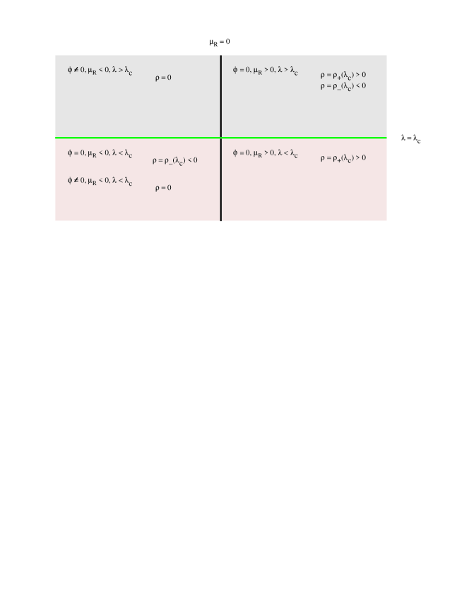
Figure 2: (Color online) Phase structure of the supersymmetric $O(N)$ model at zero temperature in the large-$N$ approximation. We plot $\mu_{R}$ on the $x$-axis and $\lambda>0$ on the $y$-axis, and have defined $\rho_{\pm}(\lambda_{c})=\mu_{R}/\bigl{(}1\pm\lambda/\lambda_{c}\bigr{)}$.

The effective potential at finite temperature is worked out in Appendix C. From Eq. (203), we have:

$$V_{N}(\phi,\rho,R;\beta)=\frac{1}{2}\,m^{2}\,\phi^{2}+\frac{2}{\lambda}\,R\,(\,\mu_{R}-\rho\,)\\ -\frac{1}{12\pi}\bigl{(}\,|m|^{3}-|\rho|^{3}\,\bigr{)}\\ +\frac{1}{\beta}\int_{0}^{+\infty}\frac{k\,\mathrm{d}k}{2\pi}\,\ln\biggl{[}\,\frac{1-\exp(-\beta\omega_{k})}{1+\exp(-\beta\omega^{\prime}_{k})}\biggr{]}\>.$$ (108)

At the minimum of the potential, $\rho$ and $R$ satisfy the gap equations (189) and (C) at finite temperature:

$$\rho =\mu_{R}+\frac{\lambda}{4}\Bigl{\{}\phi^{2}-\frac{|m|}{4\pi}-\frac{1}{2\pi\beta}\ln\bigl{[}1-\exp(-\beta|m|)\bigr{]}\Bigl{\}}$$ (109a)

$$R =\frac{\lambda}{2}\,\rho\,\Bigl{\{}\,\phi^{2}-\frac{1}{2\pi\beta}\,\Bigl{\{}\,\ln\bigl{[}\,2\sinh(\beta|m|/2)\bigr{]}$$

$$\qquad\qquad-\ln\bigl{[}\,2\cosh(\beta|\rho|/2)\bigr{]}\,\Bigr{\}}\,\Bigr{\}}\>.$$ (109b)

Noting that $R=m^{2}-\rho^{2}$, these two equations can be combined to give $m^{2}$ as a function of $\rho$ :

$$m^{2} =3\,\rho^{2}-2\,\rho\,\mu_{R}$$ (110)

$$\qquad+\frac{\lambda}{8\pi}\,|\rho|\,\rho+\frac{\lambda}{4\pi\beta}\,\ln\bigl{[}\,1+\exp(-\beta|\rho|)\,\bigr{]}\>,$$

so that at the minimum, the potential can be written as:

$$V_{N} (\phi,\rho,m;\beta)\!=\!\frac{1}{2}\rho^{2}\phi^{2}\!+\!\frac{1}{24\pi}\bigl{(}\,|m|\!-\!|\rho|\,\bigr{)}^{2}(|m|\!+\!2|\rho|)$$

$$+\frac{m^{2}-\rho^{2}}{4\pi\beta}\,\ln\bigl{[}\,1-\exp(-\beta|m|)\,\bigr{]}$$

$$+\frac{1}{\beta}\int_{0}^{+\infty}\frac{k\,\mathrm{d}k}{2\pi}\,\ln\biggl{[}\,\frac{1-\exp(-\beta\omega_{k})}{1+\exp(-\beta\omega^{\prime}_{k})}\biggr{]}\>.$$ (111)

III.3 Hartree approximation

For the Hartree approximation, the gap equation (45c) becomes:

$$\rho(t) =\mu+3\lambda/4\,\bigl{[}\,\phi^{2}(t)+g_{0}(t,t)/i\,\bigr{]}\>,$$ (112a)

$$R(t) =3\lambda/2\,\Bigl{\{}\,\rho(t)\,\bigl{[}\,\phi^{2}(t)+g_{0}(t,t)/i\,\bigr{]}-\frac{\lambda}{2}\phi^{4}$$

$$\qquad\qquad\qquad+\mathrm{Tr}[\,g_{2}(t,t)\,]/i\,\Bigr{\}}\>.$$ (112b)

Here, we have set $N=1$. The Green function in the vacuum is the same as in the large-$N$ approximation, and is given by Eq. (83). So the gap equations in the vacuum are given by:

$$\rho =\mu+\frac{3\lambda}{4}\,\Bigl{[}\,\phi^{2}+\int^{\Lambda}\frac{\mathrm{d}^{3}k}{(2\pi)^{3}}\,\frac{1}{k^{2}+\rho^{2}+R}\,\Bigr{]}\>,$$ (113a)

$$R =\frac{3\lambda}{2}\rho\Bigl{[}\phi^{2}-\frac{\lambda}{2}\,\phi^{4}$$ (113b)

$$\qquad+\int\frac{\mathrm{d}^{3}k}{(2\pi)^{3}}\,\Bigl{(}\frac{1}{k^{2}+\rho^{2}+R}-\frac{1}{k^{2}+\rho^{2}}\Bigr{)}\Bigr{]}\>.$$

We renormalize Eq. (113a) by subtracting it about the point $k^{2}=0$ with a renormalized constant $\mu_{R}$ defined by:

$$\mu_{R}=\mu+\frac{3\lambda}{4}\int^{\Lambda}\frac{\mathrm{d}^{3}k}{(2\pi)^{3}}\,\frac{1}{k^{2}}\>.$$ (114)

This gives the renormalized gap equation:

$$\rho =\mu_{R}+\frac{3\lambda}{4}\,\Bigl{(}\,\phi^{2}-\frac{1}{4\pi}\,|m|\,\Bigr{)}\>,$$ (115)

where $m^{2}=\rho^{2}+R$. Eq. (113b) is finite, and yields:

$$R=\frac{3\lambda}{2}\,\rho\,\Bigl{[}\,\phi^{2}-\frac{1}{4\pi}\,(\,|m|-|\rho|\,)\,\Bigr{]}-\frac{3\lambda^{2}}{4}\,\phi^{4}\>.$$ (116)

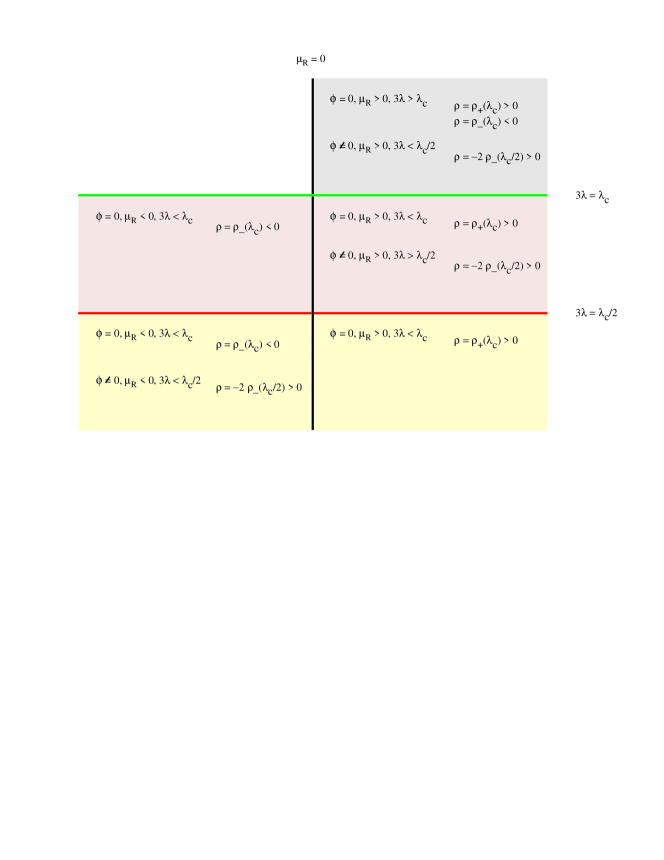
Figure 3: (Color online) Phase structure of the supersymmetric $O(N)$ model at zero temperature in the Hartree approximation. We plot $\mu_{R}$ on the $x$-axis and $\lambda>0$ on the $y$-axis, and have defined here, we use the notation $\rho_{\pm}(\lambda_{c})=\mu_{R}/\bigl{(}1\pm 3\lambda/\lambda_{c}\bigr{)}$.

From Eq. (46), and using (69) and (70), and the renormalization prescription (114), the Hartree effective potential for $N=1$ is given by:

$$V_{H}(\phi,F,\rho,R)=V_{\text{c}}(\phi,F,\rho,R)+V_{\text{q}}(\rho,R)\>,$$ (117)

The classical part is now given by

$$V_{\text{c}}(\phi,F,\rho,R)=\rho\,\phi\,F-\frac{1}{2}\,F^{2}+\frac{1}{2}\,R\,\phi^{2}\\ -\frac{\lambda}{2}\,F\,\phi^{3}+\frac{2}{3\lambda}\,R\,(\,\mu_{R}-\rho\,)\>.$$ (118)

The quantum part is the same as in the large-$N$ case and is given by Eq. (99). So the effective potential in the vacuum for the Hartree approximation is given by:

$$V_{H}(\phi,F,\rho,R)=\rho\,\phi\,F-\frac{1}{2}\,F^{2}+\frac{1}{2}\,R\,\phi^{2}-\frac{\lambda}{2}\,F\,\phi^{3}\\ +\frac{2}{3\lambda}\,R\,(\,\mu_{R}-\rho\,)-\frac{1}{12\pi}\,\bigl{(}\,|m|^{3}-|\rho|^{3}\,\bigr{)}\>.$$ (119)

The minimum of the potential is when

$$F=\rho\,\phi-\frac{\lambda}{2}\,\phi^{3}\>,$$ (120)

at which point, the effective potential is given by:

$$V_{H}(\phi,\rho,R)=\frac{1}{2}\,m^{2}\,\phi^{2}-\frac{\lambda}{2}\,\rho\,\phi^{4}+\frac{\lambda^{2}}{8}\,\phi^{6}\\ +\frac{2}{3\lambda}\,R\,(\,\mu_{R}-\rho\,)-\frac{1}{12\pi}\,\bigl{(}\,|m|^{3}-|\rho|^{3}\,\bigr{)}\>.$$ (121)

Minimizing with respect to $\rho$ and $R$ again give the gap equations, (115) and (116). At the minimum, the effective potential can be written as

$$V_{H}(\phi,\rho)=\frac{1}{2}\,\rho^{2}\,\phi^{2}-\frac{\lambda}{2}\,\rho\,\phi^{4}+\frac{\lambda^{2}}{8}\,\phi^{6}\\ +\frac{1}{24\pi}(\,|m|-|\rho|\,)^{2}\,(\,|m|+2\,|\rho|\,)\>,$$ (122)

where we note the terms proportional to $\phi^{4}$ and $\phi^{6}$ present in the Hartree potential in contrast with the leading-order large-$N$ result (see Eq. (103)).

The minimum of (122) with respect to $\phi$ occurs when

$$\frac{\partial V_{H}(\phi,\rho)}{\partial\phi}=\Bigl{\{}\,\rho^{2}-2\lambda\rho\,\phi^{2}+\frac{3}{4}\lambda^{2}\phi^{4}\,\Bigr{\}}\,\phi=0\>,$$ (123)

which gives the solutions $\phi=0$ and $\phi=\phi_{\pm}$, where:

$$\phi_{+}^{2}=\frac{2|\rho|}{\lambda}\>,\qquad\phi_{-}^{2}=\frac{2|\rho|}{3\lambda}\>.$$ (124)

Unlike Eq. (101) we notice that spontaneous symmetry breaking does not lead to massless particles. This apparent defect in the case of the Hartree approximation of the $O(N)$ model has been discussed extensively in the literature; a review of the literature and the solution of how to restore the Goldstone theorem in this approximation has recently been given in Ref. Ivanov et al. (2005a, b).

When $\phi=0$, the minimum of the potential is

$$V_{H}(\phi=0)=\frac{1}{24\pi}(\,|m|-|\rho|\,)^{2}\,(\,|m|+2\,|\rho|\,)\>,$$ (125)

which will reach its lowest value for $m=|\rho|$, or $R=0$. When $\phi\neq 0$, Eq. (124) requires that the minimum occurs at positive $\rho$, so that at the minimum

$$V_{H}(\phi\neq 0,\rho)=V_{H}(\phi=0,\rho)-\frac{\rho^{2}}{9}\,\Bigl{(}\phi^{2}-\frac{2\rho}{\lambda}\,\Bigl{)}\>.$$ (126)

From this we determine

$$V_{H}(\phi_{+},\rho) =V_{H}(\phi=0,\rho)\>,$$ (127)

$$V_{H}(\phi_{-},\rho) =V_{H}(\phi=0,\rho)+\frac{4\rho^{3}}{27\lambda}\>.$$ (128)

We conclude that an absolute minimum is located at $\phi_{+}$, which has the same energy as the minimum at $\phi=0$.

When $\phi=0$, the phase structure of the vacuum in the Hartree approximation is the same as in the leading order large-$N$ case, with the replacement $\lambda\rightarrow 3\lambda$. When $\phi\neq 0$, however, the phase structure in the Hartree approximation is different. We have

$$m=\rho=\frac{2\mu_{R}}{(3\lambda)/(8\pi)-1}>0\>,$$ (129)

which can be satisfied if either $\mu_{R}>0$ and $3\lambda>\lambda_{c}/2=8\pi$, or $\mu_{R}<0$ and $\lambda<\lambda_{c}/2$.

So, even though the phase structure of the leading-order large N and the Hartree approximation for $N=1$ obey the same equations when the symmetry is not broken, for the broken-symmetry case the two theories are quite different. The Hartree approximation yields finite masses for the fermion and boson masses, whereas in the leading-order large N the particles are massless in the broken-symmetry phase for $N=1$. Furthermore the degenerate ground-state structure differs in the two theories. We summarize the Hartree results in Fig. 3.

For completeness, we note here that the effective potential at finite temperature in the Hartree approximation, is obtained as

$$V_{H}(\phi,\rho,R;\beta)=\frac{1}{2}\,m^{2}\,\phi^{2}-\frac{\lambda}{2}\,\rho\,\phi^{4}+\frac{\lambda^{2}}{8}\,\phi^{6}\\ +\frac{2}{3\lambda}\,R\,(\,\mu_{R}-\rho\,)-\frac{1}{12\pi}\,\bigl{(}\,|m|^{3}-|\rho|^{3}\,\bigr{)}\\ +\frac{1}{\beta}\int_{0}^{+\infty}\frac{k\,\mathrm{d}k}{2\pi}\,\ln\biggl{[}\,\frac{1-\exp(-\beta\omega_{k})}{1+\exp(-\beta\omega^{\prime}_{k})}\biggr{]}\>.$$ (130)

At the minimum of the potential, $\rho$ and $R$ satisfy the finite temperature gap equations:

$$\rho=\mu_{R}+\frac{3\lambda}{4}\Bigl{\{}\phi^{2}\!-\!\frac{|m|}{4\pi}\!-\!\frac{1}{2\pi\beta}\ln\bigl{[}1-\exp(-\beta|m|)\bigr{]}\Bigl{\}}$$ (131a)

$$R=\frac{3\lambda}{2}\rho\Bigl{\{}\phi^{2}-\frac{\lambda}{2}\phi^{4}$$ (131b)

$$-\!\frac{1}{2\pi\beta}\Bigl{\{}\ln\bigl{[}\,2\sinh(\beta|m|/2)\bigr{]}\!-\!\ln\bigl{[}\,2\cosh(\beta|\rho|/2)\bigr{]}\Bigr{\}}\Bigr{\}}\>.$$

Finally, at the minimum, the potential can be written as:

$$V_{\mathrm{eff}} (\phi,\rho,m;\beta)=\frac{1}{2}\rho^{2}\phi^{2}-\frac{\lambda}{2}\,\rho\,\phi^{4}+\frac{\lambda^{2}}{8}\,\phi^{6}$$

$$+\frac{1}{24\pi}\bigl{(}\,|m|-|\rho|\,\bigr{)}^{2}(|m|+2|\rho|)$$

$$+\frac{m^{2}-\rho^{2}}{4\pi\beta}\,\ln\bigl{[}\,1-\exp(-\beta|m|)\,\bigr{]}$$

$$+\frac{1}{\beta}\int_{0}^{+\infty}\frac{k\,\mathrm{d}k}{2\pi}\,\ln\biggl{[}\,\frac{1-\exp(-\beta\omega_{k})}{1+\exp(-\beta\omega^{\prime}_{k})}\biggr{]}\>.$$ (132)

IV Conclusions

We have computed the effective potentials for a three-dimensional supersymmetric $\Phi^{4}$ model in the large-$N$ and Hartree approximations at zero temperature and at finite temperature. Both models lead to a rich degenerate ground-state structure. We find that the ground state preserves supersymmetry but can have different structure depending on the choice of coupling constant, renormalized mass and the approximation scheme. One interesting choice of parameters leads to the coexistence of a phase with broken and unbroken $O(N)$ symmetry (or parity symmetry if $N=1$). The existence of this situation leads to the interesting question of which vacuum an initial state prepared at high temperature will relax into. This will be the subject of a future investigation. Another interesting question is whether the resummed next to leading order in large-$N$ approximation obtained from the self consistent Schwinger-Dyson equations will lift the degeneracy of the vacuum. The main point of this paper was to present the conceptual (and calculational) framework for doing dynamical simulations in supersymmetric quantum field theories.

Appendix A Majorana representation in 2+1 dimensions

In three dimensions, we can choose the Dirac $\gamma$-matrices to satisfy a two-dimensional Clifford algebra:

$$\{\,\gamma^{\mu},\gamma^{\nu}\,\}=\gamma^{\mu}\gamma^{\nu}+\gamma^{\nu}\gamma^{\mu}=2\,\eta^{\mu\nu}\>,$$ (133)

with $\eta^{\mu\nu}=\text{diag}(1,-1,-1)$. The Majorana representation in 2+1 dimensions is given by the choice:

$$\gamma^{0} =\phantom{-}(\,\gamma^{0}\,)^{\dagger}=\phantom{i}\sigma^{2}=\begin{pmatrix}0&-i\\ i&0\end{pmatrix}\>,$$ (134)

$$\gamma^{1} =-(\,\gamma^{1}\,)^{\dagger}=i\sigma^{3}=\begin{pmatrix}i&0\\ 0&-i\end{pmatrix}\>,$$ (135)

$$\gamma^{2} =-(\,\gamma^{2}\,)^{\dagger}=i\sigma^{1}=\begin{pmatrix}0&i\\ i&0\end{pmatrix}\>.$$ (136)

With these choices, $(\,\gamma^{\mu}\,)^{\ast}=-\gamma^{\mu}$, and $(\,\gamma^{\mu}\,)^{\dagger}=-(\,\gamma^{\mu}\,)^{T}$, which is just the opposite of the situation for the Weyl representation. $\beta$, $\gamma^{5}$, the Hermitian conjugate ($\mathcal{C}$) and complex conjugate ($\hat{\mathcal{C}}$) operations are defined by:

$$\beta\,\gamma^{\mu}\,\beta =(\,\gamma^{\mu}\,)^{\dagger}\>,$$ (137)

$$\gamma^{5}\,\gamma^{\mu}\,\gamma^{5} =-\gamma^{\mu}\>.$$ (138)

$$\mathcal{C}\,\gamma^{\mu}\,\mathcal{C}^{-1} =-(\,\gamma^{\mu}\,)^{T} =(\,\gamma^{\mu}\,)^{\dagger}$$ (139)

$$\hat{\mathcal{C}}\,\gamma^{\mu}\,\hat{\mathcal{C}}^{-1} =-(\,\gamma^{\mu}\,)^{\ast} =\gamma^{\mu}\>.$$ (140)

From which we take:

$$\beta =(\,\beta\,)^{\dagger}=-(\,\beta\,)^{T}=-(\,\beta\,)^{\ast}=(\,\beta\,)^{-1}$$

$$=\gamma^{0}=\begin{pmatrix}0&-i\\ i&0\end{pmatrix}\>,$$ (141)

$$\gamma^{5} =(\,\gamma^{5}\,)^{\dagger}=(\,\gamma^{5}\,)^{T}=(\,\gamma^{5}\,)^{\ast}=(\,\gamma^{5}\,)^{-1}$$

$$=-\gamma^{0}\gamma^{1}=\begin{pmatrix}0&1\\ 1&0\end{pmatrix}\>.$$ (142)

$$\mathcal{C} =(\,\mathcal{C}\,)^{\dagger}=-(\,\mathcal{C}\,)^{T}=-(\,\mathcal{C}\,)^{\ast}=(\,\mathcal{C}\,)^{-1}$$

$$=\beta=\begin{pmatrix}0&-i\\ i&0\end{pmatrix}\>,$$ (143)

$$\hat{\mathcal{C}} =(\,\hat{\mathcal{C}}\,)^{\dagger}=(\,\hat{\mathcal{C}}\,)^{T}=(\,\hat{\mathcal{C}}\,)^{\ast}=(\,\hat{\mathcal{C}}\,)^{-1}$$

$$=\mathcal{C}\beta=\begin{pmatrix}1&0\\ 0&1\end{pmatrix}\>.$$ (144)

With these selections, $\gamma^{5}$, $\beta$, and $\mathcal{C}$ obey the relations:

$$\{\,\gamma^{5},\beta\,\}=[\,\beta,\mathcal{C}\,]=\{\,\mathcal{C},\gamma^{5}\,\}=0\>.$$ (145)

These commutation and anticommutation relations differ from the situation in 3+1 dimensions. We write a two-component spinor $\psi$ and $\bar{\psi}=\psi^{\dagger}\beta$ as:

$$\psi=\begin{pmatrix}\psi_{1}\\ \psi_{2}\end{pmatrix}\>,\qquad\bar{\psi}=\begin{pmatrix}i\psi_{2}^{\ast},&-i\psi_{1}^{\ast}\end{pmatrix}\>.$$ (146)

Then a Majorana spinor satisfies:

$$\psi=\psi_{c}=\hat{\mathcal{C}}\,\psi^{\ast}=\psi^{\ast}\>,$$ (147)

which means that Majorana spinors are real, $\psi_{1}^{\ast}=\psi_{1}$ and $\psi_{2}^{\ast}=\psi_{2}$.

Appendix B Majorana Grassmann quantities

In the Majorana representation, we define a real two-component column Majorana Grassmann spinor $\theta$ by:

$$\theta=\begin{pmatrix}\theta_{1}\\ \theta_{2}\end{pmatrix}\>,$$ (148)

with $\theta_{1}$ and $\theta_{2}$ real. The imaginary two-component row spinor $\bar{\theta}$ is defined by:

$$\bar{\theta}=\theta^{T}\,\beta=\begin{pmatrix}i\theta_{2},&-i\theta_{1}\end{pmatrix}\equiv\begin{pmatrix}\bar{\theta}_{1},&\bar{\theta}_{2}\end{pmatrix}\>.$$ (149)

where $\bar{\theta}_{1}=i\theta_{2}$ and $\bar{\theta}_{2}=-i\theta_{1}$ are imaginary Grassmann variables. In component notation, we have:

$$\bar{\theta}_{b}=\theta_{a}\,\beta_{ab}\>,\qquad\text{and}\qquad\theta_{b}=\bar{\theta}_{a}\,\beta_{ab}\>.$$ (150)

The Grassmann variables all anticommute:

$$\{\,\theta_{a},\theta_{b}\,\}=\{\,\theta_{a},\bar{\theta}_{b}\,\}=\{\,\bar{\theta}_{a},\theta_{b}\,\}=\{\,\bar{\theta}_{a},\bar{\theta}_{b}\,\}=0\>.$$ (151)

This means that $\theta_{a}^{2}=0$ and $\bar{\theta}_{a}^{2}=0$ (no sum over $a$ required here). We find the useful relations:

$$\bar{\theta}\cdot\theta=i\,(\,\theta_{2}\theta_{1}-\theta_{1}\theta_{2}\,)=-2i\,\theta_{1}\theta_{2}\>,\ \bar{\theta}_{a}\theta_{b}=\frac{1}{2}\,\bar{\theta}\cdot\theta\>\delta_{ab}\>.$$ (152)

Grassmann derivatives operators are defined by:

$$\partial_{a}=\frac{\partial}{\partial\theta_{a}}\>,\qquad\text{and}\quad\bar{\partial}_{a}=\frac{\partial}{\partial\bar{\theta}_{a}}\>,$$ (153)

so that $\partial_{1}$ and $\partial_{2}$ are real and $\bar{\partial}_{1}=-i\partial_{2}$ and $\bar{\partial}_{2}=i\partial_{1}$ are imaginary. We follow convention and reverse the definition of row and column matrices for the derivatives, and write:

$$\bar{\partial}\equiv\begin{pmatrix}\bar{\partial}_{1}\\ \bar{\partial}_{2}\end{pmatrix}\>,\qquad\text{and}\quad\partial\equiv\begin{pmatrix}\partial_{1}&\partial_{2}\end{pmatrix}=\bar{\partial}^{T}\,\beta\>.$$ (154)

In component notation, we have:

$$\partial_{b}=\bar{\partial}_{a}\,\beta_{ab}\>,\qquad\text{and}\quad\bar{\partial}_{b}=\partial_{a}\,\beta_{ab}\>.$$ (155)

So we find:

$$\partial_{a}\theta_{b}=\bar{\partial}_{a}\bar{\theta}_{b}=\delta_{ab}\>,$$ (156)

$$\partial_{a}\bar{\theta}_{b}=\beta_{ab}\>,\qquad\bar{\partial}_{a}\theta_{b}=\beta_{ba}\>,$$

so that $\bar{\theta}$ is not independent of $\theta$. The differential operators obey the following anticommutator relations:

$$\{\,\partial_{a},\partial_{b}\,\}=\{\,\bar{\partial}_{a},\bar{\partial}_{b}\,\}=\{\,\partial_{a},\bar{\partial}_{b}\,\}=0\>,$$ (157)

This means that $\partial_{a}^{2}=0$ and $\bar{\partial}_{a}^{2}=0$ (no sum over $a$ required here). We also have:

$$\{\,\partial_{a},\theta_{b}\,\}=\{\,\bar{\partial}_{a},\bar{\theta}_{b}\,\}=\delta_{ab}$$ (158)

$$\{\,\partial_{a},\bar{\theta}_{b}\,\}=\beta_{ab}\,\>,\qquad\{\,\bar{\partial}_{a},\theta_{b}\,\}=\beta_{ba}\,\>.$$

It is useful to define the integration measure with a factor of $i/2$ so that we have the relations:

$$\mathrm{d}^{2}\theta=\frac{1}{2}\,\mathrm{d}\bar{\theta}_{1}\,\mathrm{d}\theta_{1}=\frac{i}{2}\,\mathrm{d}\theta_{2}\,\mathrm{d}\theta_{1}\>,$$ (159)

$$\int\mathrm{d}^{2}\theta=\int\mathrm{d}^{2}\theta\>\theta_{a}=0\>,$$

$$\int\mathrm{d}^{2}\theta\>\bar{\theta}_{a}\,\theta_{b}=\frac{1}{2}\,\delta_{ab}\>,\quad\int\mathrm{d}^{2}\theta\>\bar{\theta}\cdot\theta=1\>.$$

With this convention, the Grassmann two-dimensional delta function for two anticommuting Grassmann quantities is given by:

$$\delta^{2}(\theta-\theta^{\prime}) =(\,\bar{\theta}-\bar{\theta}^{\prime}\,)\cdot(\,\theta-\theta^{\prime}\,)$$

$$=\bar{\theta}\cdot\theta-\bar{\theta}\cdot\theta^{\prime}-\bar{\theta}^{\prime}\cdot\theta+\bar{\theta}^{\prime}\cdot\theta^{\prime}$$

$$=\bar{\theta}\cdot\theta-2\,\bar{\theta}\cdot\theta^{\prime}+\bar{\theta}^{\prime}\cdot\theta^{\prime}\>.$$ (160)

If $\theta$ and $\phi$ are two anticommuting Majorana Grassmann spinors, we have the useful identities:

$$\bar{\theta}\cdot\phi=\bar{\phi}\cdot\theta\>,\qquad\bar{\theta}\cdot\gamma^{\mu}\cdot\phi=-\bar{\phi}\cdot\gamma^{\mu}\cdot\theta\>,$$ (161)

$$\bar{\theta}_{a}\,\theta_{b}=\delta_{a,b}\,(\bar{\theta}\cdot\theta)/2\>,\qquad\bar{\theta}\cdot\gamma^{\mu}\cdot\theta=0\>,$$ (162)

$$\partial_{a}(\bar{\theta}\cdot\theta)=(\partial_{a}\bar{\theta}_{b})\,\theta_{b}-\bar{\theta}_{b}\,(\partial_{a}\bar{\theta}_{b})=-2\,\bar{\theta}_{a}\>,$$ (163)

$$\bar{\partial}_{a}(\bar{\theta}\cdot\theta)=(\bar{\partial}_{a}\bar{\theta}_{b})\,\theta_{b}-\bar{\theta}_{b}\,(\bar{\partial}_{a}\bar{\theta}_{b})=+2\,\theta_{a}\>,$$ (164)

$$(\partial\cdot\bar{\partial})\,(\bar{\theta}\cdot\theta)=4\>.$$ (165)

The supercharge generators $Q$ and $\bar{Q}$ and the superderivative operators $D$ and $\bar{D}$ are defined by:

$$Q =-\bar{\partial}-i\,\partial\!\!\!/\cdot\theta\>, \qquad D =+\bar{\partial}-i\,\partial\!\!\!/\cdot\theta\>,$$ (166)

$$\bar{Q} =+\partial+i\,\bar{\theta}\cdot\partial\!\!\!/\>, \qquad\bar{D} =-\partial+i\,\bar{\theta}\cdot\partial\!\!\!/\>.$$

where we have used the Dirac slash notation, $\partial\!\!\!/=\gamma^{\mu}\partial_{\mu}$. The $Q$ operators obey the superalgebra:

$$\{\,Q_{a},\bar{Q}_{b}\,\}=-2i\,(\,\gamma^{\mu}\,)_{ab}\,\partial_{\mu}\>,$$ (167)

$$\qquad\{\,Q_{a},Q_{b}\,\}=0\>,\qquad\{\,\bar{Q}_{a},\bar{Q}_{b}\,\}=0\>.$$

Thus we find:

$$Q\cdot Q=\bar{Q}\cdot\bar{Q}=0\>,$$ (168)

$$Q\cdot\bar{Q}+\bar{Q}\cdot Q=-2i\,\mathrm{Tr}\{\gamma^{\mu}\}\,\partial_{\mu}=0\>.$$

The $D$ operators satisfy a similar superalgebra but with a reversed sign:

$$\{\,D_{a},\bar{D}_{b}\,\}=2i\,(\,\gamma^{\mu}\,)_{ab}\,\partial_{\mu}\>.$$ (169)

$$\{\,D_{a},D_{b}\,\}=0\>,\quad\{\,\bar{D}_{a},\bar{D}_{b}\,\}=0\>,$$

So we find:

$$D\cdot D=\bar{D}\cdot\bar{D}=0\>,$$ (170)

$$D\cdot\bar{D}+\bar{D}\cdot D=2i\,\mathrm{Tr}\{\gamma^{\mu}\}\,\partial_{\mu}=0\>.$$

The $Q$ and $D$ operators anticommute:

$$\{\,D_{a},Q_{b}\,\} =\{\,\bar{D}_{a},\bar{Q}_{b}\,\}$$ (171)

$$=\{\,D_{a},\bar{Q}_{b}\,\}=\{\,\bar{D}_{a},Q_{b}\,\}=0\>.$$

The operators $Q$ and $D$ are related by:

$$Q=D-2\bar{\partial}\>,\qquad\bar{Q}=\bar{D}+2\partial\>.$$ (172)

We also find:

$$\bar{D}\cdot D =\bigl{(}\,-\partial+i\,\bar{\theta}\cdot\gamma^{\mu}\,\partial_{\mu}\,\bigr{)}\cdot\bigl{(}\,\bar{\partial}-i\,\gamma^{\nu}\cdot\theta\,\partial_{\nu}\,\bigr{)}$$

$$=-\partial\cdot\bar{\partial}-i\,\bigl{(}\,\partial\cdot\gamma^{\mu}\cdot\theta-\bar{\theta}\cdot\gamma^{\mu}\cdot\bar{\partial}\,\bigr{)}\,\partial_{\mu}$$

$$\qquad+\bar{\theta}\cdot\gamma^{\mu}\cdot\gamma^{\nu}\cdot\theta\,\partial_{\mu}\,\partial_{\nu}$$ (173)

$$=-\partial\cdot\bar{\partial}+2i\,\bar{\theta}\cdot\gamma^{\mu}\cdot\bar{\partial}\,\partial_{\mu}+(\bar{\theta}\cdot\theta)\,\square\>,$$

where $\partial\cdot\bar{\partial}=\partial_{1}\,\bar{\partial}_{1}+\partial_{2}\,\bar{\partial}_{2}$ and $\square=\partial_{t}^{2}-\partial_{x}^{2}$. From Eq. (B), we find:

$$\bar{D}\cdot D\,\delta(\theta,\theta^{\prime})=-4\,e^{i\bar{\theta}\cdot\partial\!\!\!/\cdot\theta^{\prime}}\>,$$ (174)

Appendix C Temperature dependent supergreen functions

We use a complex time formalism for the temperature dependent Green functions. The superperiodic boundary condition on the superfield is then given by:

$$\Phi_{i}(\mathbf{x},\beta;\theta)=\Phi_{i}(\mathbf{x},0;-\theta)\>.$$ (175)

So the fields and Green functions can be expanded in a Fourier series for the imaginary time variable, and a Fourier integral for the space variable. We consider here only spacial homogeneous systems. Thus for the fields, we write:

$$\Phi(\mathbf{x},\tau;\theta)=\int\frac{\mathrm{d}^{2}k}{(2\pi)^{2}}\,\frac{e^{i\mathbf{k}\cdot\mathbf{x}}}{\beta}\sum_{n=-\infty}^{+\infty}\biggl{\{}\,\tilde{\phi}_{n}(k)\,e^{i\omega_{n}\tau}$$

$$+\bar{\theta}\cdot\tilde{\psi}_{n}(k)\,e^{i\omega^{\prime}_{n}\tau}+\frac{1}{2}\,(\bar{\theta}\cdot\theta)\,\tilde{F}_{n}(k)\,e^{i\omega_{n}\tau}\,\biggr{\}}\>,$$ (176)

where $\beta=1/k_{\text{B}}T$ and $\omega_{n}$ and $\omega^{\prime}_{n}$ are the Bose and Fermi Matsubara frequencies:

$$\begin{split}\omega_{n}&=\pi\,2n/\beta\>,\qquad\text{for boson fields.}\\ \omega^{\prime}_{n}&=\pi\,(2n+1)/\beta\>,\qquad\text{for fermi fields.}\end{split}$$ (177)

The Green functions are expanded according to:

$$G(x,\tau,\theta; x^{\prime},\tau^{\prime},\theta^{\prime})=\int\frac{\mathrm{d}^{2}k}{(2\pi)^{2}}\,\frac{1}{\beta}$$ (178)

$$\times\sum_{n=-\infty}^{+\infty}\tilde{G}_{n}(\mathbf{k};\theta,\theta^{\prime})\,e^{i[\,\mathbf{k}\cdot(\mathbf{x}-\mathbf{x}^{\prime})+\omega_{n}(\tau-\tau^{\prime})\,]}\>.$$

$\tilde{G}_{n}(\mathbf{k};\theta,\theta^{\prime})$ satisfies:

$$\Bigl{[}-\partial\cdot\bar{\partial}+2i\,\bar{\theta}\cdot k\!\!\!/^{\prime}_{n}\cdot\bar{\partial}+\bar{\theta}\cdot\theta\,k_{n}^{2}+\chi(\theta)\Bigr{]}\tilde{G}_{n}(\mathbf{k};\theta,\theta^{\prime})$$

$$=\ \delta^{2}(\theta-\theta^{\prime})\>.$$ (179)

Here $k_{n}^{\mu}=(\omega_{n},\mathbf{k})$ and $k^{\prime}_{n}{}^{\mu}=(\omega^{\prime}_{n},\mathbf{k})$ are the Euclidean vectors, with $k\!\!\!/=\gamma^{\mu}(k_{n})_{\mu}$ and $k\!\!\!/^{\prime}=\gamma^{\mu}(k^{\prime}_{n})_{\mu}$. We find:

$$\tilde{G}_{n}(\mathbf{k};\theta,\theta^{\prime})=\bar{\theta}\cdot\frac{ik\!\!\!/^{\prime}_{n}-\rho}{k^{\prime}_{n}{}^{2}+\rho^{2}}\cdot\theta^{\prime}$$ (180)

$$+\frac{1+\tfrac{1}{2}\,(\,\bar{\theta}\cdot\theta+\bar{\theta}^{\prime}\cdot\theta^{\prime}\,)\,\rho-\tfrac{1}{4}\,\bar{\theta}\cdot\theta\,\bar{\theta}^{\prime}\cdot\theta^{\prime}\,(\,k_{n}^{2}+\rho^{2}\,)\,}{k_{n}^{2}+\rho^{2}+R}\>,$$

in agreement with MZJ Moshe and Zinn-Justin (2003)[Eq. (2.7)]. The diagonal elements of $\tilde{G}_{n}(\mathbf{k};\theta,\theta^{\prime})$ are given by:

$$\tilde{G}_{n}(\mathbf{k};\theta,\theta)=\frac{1+\bar{\theta}\cdot\theta\,\rho}{k_{n}^{2}+\rho^{2}+R}-\frac{\bar{\theta}\cdot\theta\,\rho}{k^{\prime}_{n}{}^{2}+\rho^{2}}\>.$$ (181)

We define:

$$\omega_{k}=\sqrt{k^{2}+\rho^{2}+R}\>,$$ (182)

$$\omega^{\prime}_{k}=\sqrt{k^{2}+\rho^{2}}\>.$$ (183)

Then the sum over $n$ is given by:

$$\begin{split}\sum_{n=-\infty}^{+\infty}\frac{1}{\omega_{n}^{2}+\omega_{k}^{2}}&=\frac{\beta}{2\,\omega_{k}}\,\coth(\beta\omega_{k}/2)\\ &=\frac{\beta}{2\,\omega_{k}}\,\Bigl{[}\,1+2\,n_{-}(\beta\omega_{k})\,\Bigr{]}\>,\\ \sum_{n=-\infty}^{+\infty}\frac{1}{\omega^{\prime}_{n}{}^{2}+\omega^{\prime}_{k}{}^{2}}&=\frac{\beta}{2\,\omega^{\prime}_{k}}\,\tanh(\beta\omega^{\prime}_{k}/2)\\ &=\frac{\beta}{2\,\omega^{\prime}_{k}}\,\Bigl{[}\,1-2\,n_{+}(\beta\omega^{\prime}_{k})\,\Bigr{]}\>,\end{split}$$ (184)

where we have $n_{\pm}(x)=[{e^{x}\pm 1}]^{-1}$. So

$$\frac{1}{\beta}\sum_{n=-\infty}^{+\infty} \tilde{G}_{n}(\mathbf{k};\theta,\theta)=\frac{\coth(\beta\omega_{k}/2)}{2\omega_{k}}$$ (185)

$$+\bar{\theta}\cdot\theta\,\biggl{[}\,\frac{\rho\coth(\beta\omega_{k}/2)}{2\omega_{k}}-\frac{\rho\tanh(\beta\omega^{\prime}_{k}/2)}{2\omega^{\prime}_{k}}\,\biggr{]}$$

For the large-$N$ approximation, the thermal gap equation becomes:

$$\chi(\theta)\!=\!2\mu\!+\!\frac{\lambda}{2}\sum_{i}\Phi_{i}^{2}(\theta)\!+\!\frac{\lambda}{2}\int\frac{\mathrm{d}^{2}k}{(2\pi)^{2}}\biggl{\{}\frac{\coth(\beta\omega_{k}/2)}{2\omega_{k}}$$

$$+\bar{\theta}\cdot\theta\biggl{[}\frac{\rho\coth(\beta\omega_{k}/2)}{2\omega_{k}}-\frac{\rho\tanh(\beta\omega^{\prime}_{k}/2)}{2\omega^{\prime}_{k}}\biggr{]}\biggr{\}}$$ (186)

from which we find, for $N=1$:

$$\rho =\mu+\frac{\lambda}{4}\phi^{2}+\frac{\lambda}{4}\int^{\Lambda}\frac{\mathrm{d}^{2}k}{(2\pi)^{2}}\frac{\coth(\beta\omega_{k}/2)}{2\omega_{k}}\>,$$ (187a)

$$R =\frac{\lambda}{2}\,\phi\,F$$ (187b)

$$+\frac{\lambda}{2}\int\frac{\mathrm{d}^{2}k}{(2\pi)^{2}}\,\biggl{[}\,\frac{\rho\coth(\beta\omega_{k}/2)}{2\omega_{k}}-\frac{\rho\tanh(\beta\omega^{\prime}_{k}/2)}{2\omega^{\prime}_{k}}\,\biggr{]}$$

Here we have used a finite cutoff $\Lambda$ so as to make the integral in Eq. (187a) finite. We renormalize this by defining:

$$\mu_{R}=\mu+\frac{\lambda}{4}\int_{0}^{\Lambda}\frac{k\,\mathrm{d}k}{2\pi}\,\frac{1}{2\sqrt{k^{2}}}\>.$$ (188)

so that Eq. (187a) becomes:

$$\begin{split}\rho&=\mu_{R}+\frac{\lambda}{4}\,\phi^{2}-\frac{\lambda}{8\pi\beta}\,\ln\bigl{[}\,2\sinh(\beta m/2)\bigr{]}\>,\end{split}$$ (189)

where again $m^{2}=\rho^{2}+R$. Eq. (187b) is finite, and becomes:

$$\begin{split}&R=\frac{\lambda}{2}\,\phi\,F\\ &-\frac{\lambda\rho}{4\pi\beta}\,\Bigl{\{}\,\ln\bigl{[}2\sinh(\beta m/2)\bigr{]}-\ln\bigl{[}2\cosh(\beta\rho/2)\bigr{]}\,\Bigr{\}}\>.\end{split}$$

Multiplying (189) by $2\rho$ and subtracting it from (C) yields:

$$R=\rho\,\Bigl{\{}\,2\,(\rho-\mu_{R})-\frac{\lambda}{4\pi\beta}\,\ln\bigl{[}2\cosh(\beta\rho/2)\bigr{]}\,\Bigr{\}}\>,$$ (190)

along the line where $F=\rho\,\phi$.

The effective potential at finite temperature for large-$N$ is written as the sum of two terms:

$$V_{\text{eff}}(\phi,F;\rho,R;\beta)=V_{\text{c}}(\phi,F;\rho,R)+V_{\text{q}}(\rho,R;\beta)\>,$$ (191)

where the classical part is given by:

$$V_{\text{c}}(\phi,F;\rho,R)=\rho\,\phi\,F-\frac{1}{2}\,F^{2}+\frac{1}{2}\,R\,\phi^{2}+\frac{2}{\lambda}\,R\,(\,\mu_{R}-\rho\,)\>.$$ (192)

At the minimum, where $F=\rho\,\phi$, $V_{\text{c}}(\phi,\rho\,\phi;\rho,R)$ becomes:

$$V_{\text{c}}(\phi;\rho,R)=\frac{1}{2}\,m^{2}\,\phi^{2}+\frac{2}{\lambda}\,R\,(\,\mu_{R}-\rho\,)\>.$$ (193)

For the quantum part $V_{\text{q}}(\rho,R)$, we define $W_{\text{q}}(\rho,R;\theta)$ by:

$$V_{\text{q}}(\rho,R;\beta)=\int\mathrm{d}^{2}\theta\,W_{\text{q}}(\rho,R;\theta;\beta)\>.$$ (194)

For $d=3$, $W_{\text{q}}(\rho,R;\theta)$ is given by:

$$W_{\text{q}}(\rho,R; \theta;\beta)=\frac{1}{8\pi}\,\int_{0}^{\infty}k\,\mathrm{d}k$$ (195)

$$\times\biggl{\{}\,\frac{1}{i\beta}\,\sum_{n=-\infty}^{+\infty}\ln\bigl{[}\,\tilde{G}_{n}^{-1}(k;\theta,\theta)\,\bigr{]}-\frac{\chi(\theta)}{2\sqrt{k^{2}}}\,\biggr{\}}\>.$$

Again, we can write

$$\frac{\delta W_{\text{q}}(\rho,R;\theta;\beta)}{\delta\chi(\theta)}= W_{0}(\rho,R;\beta)+\frac{1}{2}\,\bar{\theta}\cdot\theta\,W_{1}(\rho,R;\beta)\>,$$ (196)

with

$$W_{0}(\rho,R;\beta)=-\frac{1}{4\pi\beta}\ln\bigl{[}\,2\sinh(\beta m/2)\,\bigr{]}\>,$$ (197)

and

$$W_{1}(\rho,R;\beta)=-\frac{Nrho}{2\pi\beta}\Bigl{\{}\, \ln\bigl{[}\,2\sinh(\beta m/2)\,\bigr{]}$$ (198)

$$\quad-\ln\bigl{[}\,2\cosh(\beta\rho/2)\,\bigr{]}\,\Bigr{\}}\>.$$

Again, we have

$$\delta\chi(\rho,R)=2\delta\rho+\bar{\theta}\cdot\theta\,\delta R\>,$$ (199)

so

$$\begin{split}&\delta W_{\text{q}}(\rho,R;\theta;\beta)=2\,W_{0}(\rho,R)\,\delta\rho\\ &+\bar{\theta}\cdot\theta\,\bigl{[}\,W_{0}(\rho,R;\beta)\,\delta R+W_{1}(\rho,R;\beta)\,\delta\rho\,\bigr{]}\end{split}$$ (200)

We now want to find a common function $V_{\text{q}}(\rho,R;\beta)$ such that:

$$\begin{split}\frac{\partial V_{\text{q}}(\rho,R;\beta)}{\partial R}&=W_{0}(\rho,R;\beta)\>,\\ \frac{\partial V_{\text{q}}(\rho,R;\beta)}{\partial\rho}&=W_{1}(\rho,R;\beta)\>.\end{split}$$ (201)

We can use the following identities:

$$\begin{split}\frac{\rho\,n_{-}(\beta\omega_{k})}{\omega_{k}}&=\frac{1}{\beta}\frac{\partial}{\partial\rho}\Bigl{\{}\ln\bigl{[}1-\exp(-\beta\omega_{k})\bigr{]}\Bigr{\}}\>,\\ \frac{\rho\,n_{+}(\beta\omega^{\prime}_{k})}{\omega^{\prime}_{k}}&=-\frac{1}{\beta}\frac{\partial}{\partial\rho}\Bigl{\{}\ln\bigl{[}1+\exp(-\beta\omega^{\prime}_{k})\bigr{]}\Bigr{\}}\>,\\ \frac{n_{-}(\beta\omega_{k})}{2\omega_{k}}&=\frac{1}{\beta}\frac{\partial}{\partial R}\Bigl{\{}\ln\bigl{[}1-\exp(-\beta\omega_{k})\bigr{]}\Bigr{\}}\>.\end{split}$$

So the function we seek is:

$$V_{q}(\rho,R; \beta)=\frac{1}{12\pi}\bigl{(}|\rho|^{3}-|m|^{3}\bigr{)}$$ (202)

$$+\frac{1}{2\pi\beta}\int_{0}^{+\infty}k\mathrm{d}k\,\ln\bigl{[}1-\exp(-\beta\omega_{k})\bigr{]}$$

$$-\frac{1}{2\pi\beta}\int_{0}^{+\infty}k\mathrm{d}k\,\ln\bigl{[}1+\exp(-\beta\omega^{\prime}_{k})\bigr{]}\>.$$

Thus the effective potential at finite temperature and along the line $F=\rho\,\phi$ is given by:

$$V_{\mathrm{eff}}(\phi,\rho,R; \beta)=\frac{1}{2}\,m^{2}\,\phi^{2}+\frac{2}{\lambda}\,R\,(\,\mu_{R}-\rho\,)$$ (203)

$$+\frac{1}{12\pi}\bigl{(}\,|\rho|^{3}-|m|^{3}\,\bigr{)}$$

$$+\frac{1}{2\pi\beta}\int_{0}^{+\infty}k\,\mathrm{d}k\,\ln\bigl{[}1-\exp(-\beta\omega_{k})\bigr{]}\,$$

$$-\frac{1}{2\pi\beta}\int_{0}^{+\infty}k\,\mathrm{d}k\,\ln\bigl{[}1+\exp(-\beta\omega^{\prime}_{k})\bigr{]}\,\>.$$

This expression agrees with Eq. (100) in the vacuum when $\beta\rightarrow\infty$.

References

- Wess and Bagger (1992) J. Wess and J. Bagger, Supersymmetry and Supergravity (Princeton University Press, Princeton, NJ, 1992), 2nd ed.
- Cornwall et al. (1974) J. M. Cornwall, R. Jackiw, and E. Tomboulis, Phys. Rev. D 10, 2428 (1974).
- Luttinger and Ward (1960) J. M. Luttinger and J. C. Ward, Phys. Rev. 118, 1417 (1960).
- Baym (1962) G. Baym, Phys. Rev. 127, 1391 (1962).
- Cooper et al. (2003a) F. Cooper, J. F. Dawson, and B. Mihaila, Phys. Rev. D 67, 056003 (2003a).
- Cooper et al. (2003b) F. Cooper, J. F. Dawson, and B. Mihaila, Phys. Rev. D 67, 051901(R) (2003b).
- Aarts et al. (2002) G. Aarts, D. Ahrensmeier, R. Baier, J. Berges, and J. Serreau, Phys. Rev. D 66, 045008 (2002).
- Berges and Cox (2001) J. Berges and J. Cox, Phys. Lett. B517, 369 (2001).
- Aarts and Berges (2001) G. Aarts and J. Berges, Phys. Rev. D 64, 105010 (2001).
- Berges (2002) J. Berges, Nuc. Phys. A 699, 847 (2002).
- Wilson (1973) K. G. Wilson, Phys. Rev. D 7, 2911 (1973).
- Coleman et al. (1974) S. Coleman, R. Jackiw, and H. D. Politzer, Phys. Rev. D 10, 2491 (1974).
- Schnitzer (1974) H. J. Schnitzer, Phys. Rev. D 10, 2042 (1974).
- Chang (1975) S.-J. Chang, Phys. Rev. D 12, 1071 (1975).
- Cooper et al. (1986) F. Cooper, S. Y. Pi, and P. N. Stancioff, Phys. Rev. D 34, 3831 (1986).
- Cooper and Mottola (1987) F. Cooper and E. Mottola, Phys. Rev. D 36, 3114 (1987).
- Pi and Samiullah (1987) S. Y. Pi and M. Samiullah, Phys. Rev. D 36, 3128 (1987).
- Boyanovsky et al. (1994) D. Boyanovsky, H. J. de Vega, and R. Holman, Phys. Rev. D 49, 2769 (1994).
- Blagoev et al. (2001) K. B. Blagoev, F. Cooper, J. F. Dawson, and B. Mihaila, Phys. Rev. D 64, 125003 (2001).
- Mihaila et al. (2001) B. Mihaila, J. F. Dawson, and F. Cooper, Phys. Rev. D 63, 096003 (2001).
- Das and Kaku (1978) A. Das and M. Kaku, Phys. Rev. D 18, 4540 (1978).
- Moshe and Zinn-Justin (2003) M. Moshe and J. Zinn-Justin, Nuc. Phys. B 648, 131 (2003).
- Feinberg et al. (2005) J. Feinberg, M. Moshe, and M. Smolkin, Inter. J. Mod. Phys. A 20, 4475 (2005).
- Shifman et al. (1999) M. Shifman, A. Vainshtein, and M. Voloshin, Phys. Rev. D 59, 045016 (1999).
- Ivanov et al. (2005a) Y. B. Ivanov, F. Riek, , and J. Knoll, Phys. Rev. D 71, 105016 (2005a).
- Ivanov et al. (2005b) Y. B. Ivanov, F. Riek, H. van Hees, and J. Knoll, Phys. Rev. D 72, 036008 (2005b).