Low scale Seesaw model and
Lepton Flavor Violating Rare $B$ Decays

Abstract

We study lepton flavor number violating rare $B$ decays, $b\to sl_{h}^{\pm}l_{l}^{\mp}$, in a seesaw model with low scale singlet Majorana neutrinos motivated by the resonant leptogenesis scenario. The branching ratios of inclusive decays $b\to sl_{h}^{\pm}\bar{l_{l}}^{\mp}$ with two almost degenerate singlet neutrinos at TeV scale are investigated in detail. We find that there exists a class of seesaw model in which the branching fractions of $b\to s\tau\mu$ and $\tau\to\mu\gamma$ can be as large as $10^{-10}$ and $10^{-9}$ within the reach of Super B factories, respectively, without being in conflict with neutrino mixings and mass squared difference of neutrinos from neutrino data, invisible decay width of $Z$ and the present limit of $Br(\mu\to e\gamma)$.

I Introduction

Thanks to the worldwide collaborative endeavor for $B$ factories and neutrino experiments, our understanding of the flavor mixing phenomena in quark sector as well as in lepton sector has been dramatically improved over the past few years. Even though discoveries of neutrino oscillations in solar, atmospheric and reactor experiments gave a robust evidence for the existence of non-zero neutrino masses, we do not yet understand mechanisms of how to generate the masses of neutrinos and why those masses are so small. The most attractive proposal to explain the smallness of neutrino masses is the seesaw mechanism [1, 2, 3, 4] in which super-heavy singlet particles are introduced. One of the virtues of the seesaw mechanism is to provide us with an elegant way to achieve the observed baryon asymmetry in our universe via the related leptogenesis [5]. However, the typical seesaw scale is of order $10^{10}\sim 10^{14}$ GeV, which makes it impossible to probe the seesaw mechanism at collider experiments in a foreseeable future. Moreover, the leptogenesis at such a high energy scale meets a serious problem, the so-called gravitino problem, when it realizes in supersymmetric extensions of the standard model. Thus, it may be quite desirable to achieve the seesaw mechanism as well as the leptogenesis at a rather low energy scale. In these regards, scenarios of the resonant leptogenesis, in which singlet neutrinos with masses of order $1\sim 10$ TeV are introduced, have been recently proposed [6, 7, 8, 9, 10, 11, 12, 13] Interestingly enough, the amplitudes of some flavor violating processes, which are highly suppressed in usual seesaw models with super-heavy singlet neutrinos, may be enhanced with such low scale singlet neutrinos. Thus, it is worthwhile to examine how we can probe a seesaw model with low scale singlet neutrinos at collider experiments and to find some experimental evidence for the seesaw model via probe of lepton flavor violating processes.

In this paper, within the context of a low scale seesaw model based on $SU(2)_{L}\times U(1)$ [14], we study quark and lepton flavor violating (QLFV) rare decay processes such as $b\to sl_{h}^{\pm}l_{l}^{\mp}$ and $l_{h}\to l_{l}\gamma$, where $l_{h}$ and $l_{l}$ denote heavy and light charged leptons, respectively. After the quark flavor changing neutral currents (FCNC) $b\to sl^{+}l^{-}$ had been discovered in $B$ factories [15], it has been naturally expected that the next generation experiments could probe well the lepton flavor violating (LFV) processes [1, 16, 17, 18] , which may eventually uncover the mechanism for the generation of small neutrino masses and the leptogenesis as well. Therefore, the precise predictions for those processes based on well motivated scenarios are very useful to find out if such scenarios can describe the nature correctly or not. Here we focus on the seesaw model motivated by the resonant leptogenesis scenario with two almost degenerate singlet neutrinos at TeV scale. In the context of the seesaw mechanism, lowering the singlet mass scale leads to an undesirable enhancement of the light neutrino masses unless the Dirac neutrino couplings are guaranteed to be naturally small. However, as shown in [19, 20], despite of the low mass scale of singlet Majorana neutrinos we can obtain light neutrino mass spectrum consistent with the current neutrino data by tuning the phase of the Yukawa-Dirac mass terms so that the two degenerate singlets contribute to the low energy effective Majorana mass terms destructively and the lepton number is approximately conserved. Interestingly enough, in such a scenario the sizable LFV processes and the suppression of the lepton number violation required in the effective Majorana mass for light neutrinos may coexist. We will show that the amplitudes of quark FCNC and LFV processes can be enhanced by considering some specific structure of Yukawa-Dirac and singlet Majorana mass matrices which are required to achieve the resonant leptpogenesis. We will obtain rather stringent constraints on QLFV processes by taking the constraints arisen from the invisible decay of $Z$ boson, neutrino mass-squared differences and lepton flavor mixings measured at neutrino experiments and the experimental constraints of LFV processes such as $l_{h}\to l_{l}\gamma$.

The paper is organized as follows: In section 2, we present the lepton flavor mixings of seesaw models with arbitrary number of singlet Majorana neutrinos. The analytical expressions for the branching fractions of the QLFV rare $B$ decays are presented and the model independent bound on the branching fractions is obtained. In section 3, we study the low mass scale scenarios for singlet neutrinos and build the models in which the quark FCNC and LFV processes are enhanced. We give the predictions for the QLFV processes by taking into account the various constraints. In section 4, we summarize the results.

II Lepton flavor mixig of seesaw model and QLFV rare $B$ decay

The lepton favor mixings of seesaw model are described in detail in Refs. [21, 22]. Here we extend the model to the case with arbitrary number of singlet neutinos and introduce a convenient decomposition of the Yukawa-Dirac mass term which is useful to our study. Let us start with a seesaw model described by following Lagrangian,

$${\cal L}_{m}=-y_{\nu}^{ik}\overline{L_{i}}N_{R_{k}}\tilde{\phi}-y_{l}^{i}\overline{L_{i}}l_{R_{i}}{\phi}-\frac{1}{2}\overline{N_{R_{k}}}^{c}M_{k}N_{R_{k}}+h.c.,$$ (1)

and the neutrino mass matrix

$$M_{\nu}=\left(\begin{array}[]{cc}\ 0&m_{D}\\ m_{D}^{T}&M\end{array}\right),$$ (4)

where $M$ is a $N\times N$ real diagonal singlet Majorana neutrino mass matrix and $m_{D}$ is a Dirac Yukawa mass term. Then, $(3+N)\times(3+N)$ neutrino mass matrix can be diagonalized by the mixing matrix ${\cal V}$ as,

$$M^{\rm Diag}_{\nu}={\cal V}^{\dagger}M_{\nu}{\cal V}^{\ast}.$$ (5)

If the seesaw condition, $i.e.$ $\frac{m_{D}}{M}<1$, is satisfied, $(3+N)\times(3+N)$ unitary matrix ${\cal V}$ can be approximately parameterized as,

$${\cal V}=\left(\begin{array}[]{cc}V&{m_{D}}\frac{1}{M}\\ -\frac{1}{M}m_{D}^{\dagger}V&\left(1_{N}-\frac{1}{M}{m_{D}}^{\dagger}m_{D}\frac{1}{M}\right)^{\frac{1}{2}}\end{array}\right),$$ (8)

where ${\cal V}$ satisfies unitarity to the order of $\frac{m_{D}^{2}}{M^{2}}$, and $1_{N}$ denotes an $N\times N$ unit matrix. Here $3\times 3$ submatrix $V$ is not exactly unitary and can be written [22] as

$$V=\left(1-m_{D}\frac{1}{M^{2}}m_{D}^{\dagger}\right)^{\frac{1}{2}}V_{0},$$ (9)

where $V_{0}$ is a unitary matrix which diagonalizes the effective Majorana mass term,

$$m_{eff} = -m_{D}\frac{1}{M}m_{D}^{T},$$

$$V_{0}^{\dagger}m_{eff}V_{0}^{\ast} = \mbox{Diag}[n_{1},n_{2},n_{3}],$$ (10)

where $n_{i}$ are the masses of three light neutrinos.

For convenience, we introduce the following parametrization for $m_{D}$ [23],

$$m_{D}=({\bf m_{D1},m_{D2},...m_{DN}}) = \left(\begin{array}[]{cccc}{\bf u_{1}}&{\bf u_{2}}&..&{\bf u_{N}}\end{array}\right)\left(\begin{array}[]{cccc}m_{D1}&0&0&0\\ 0&m_{D2}&0&0\\ 0&0&..&0\\ 0&0&0&m_{DN}\end{array}\right),$$ (16)

(17)

where $N$ unit vectors are introduced as,

$${\bf u_{I}}=\frac{\bf m_{DI}}{m_{DI}}~{},$$ (18)

with $m_{DI}=|{\bf m_{DI}}|$. By introducing the parameters of mass dimension $X_{I}=\frac{m_{DI}^{2}}{M_{I}}\ (I=1\sim N)$, $m_{eff}$ can be written as

$$m_{eff} = -\sum_{i=1}^{N}{\bf u_{i}}X_{i}{\bf u_{i}^{T}}.$$ (19)

The charged current is associated with $3\times(3+N)$ submatrix of ${\cal V}$. The deviation from the unitarity of $3\times 3$ matrix $V$ is given as

$$\sum_{a=1}^{3}V_{ia}V_{ja}^{\ast} = \delta_{ij}-\sum_{I=1}^{N}\frac{X_{I}}{M_{I}}{{u}_{iI}{u}_{jI}^{\ast}},$$

$$\sum_{i={\rm e,\mu,\tau}}V_{ia}V_{ib}^{\ast} = \delta_{ab}-\sum_{I=1}^{N}(V_{0}^{\dagger}U)_{bI}\frac{X_{I}}{M_{I}}(U^{\dagger}V_{0})_{Ia},$$ (20)

where $U=({\bf u_{1}},{\bf u_{2}},..,{\bf u_{N}})$.

Now we study the QLFV rare $B$ decay processes $b\to sl_{h}^{\pm}l_{l}^{\mp}$ in the context of the seesaw model we consider. We denote $l_{h}$ as a heavy lepton and $l_{l}$ as a light lepton, and the possible combinations for $(l_{h}^{\pm},l_{l}^{\mp})$ are $(\tau^{\pm},\mu^{\mp}),(\mu^{\pm},e^{\mp})$ and $(\tau^{\pm},e^{\mp})$. By separating the contributions from the light neutrinos with masses $n_{a}~{}(a=1\sim 3)$ and ones from the heavy neutrinos with masses $M_{A-3}~{}(A=4,5,...3+N)$, we can express the amplitude for $b\to sl_{h}^{-}l_{l}^{+}$ as

$$T=\frac{\sqrt{2}G_{F}\alpha_{QED}}{4\pi s_{W}^{2}}\times$$

$$\left(\overline{u_{s}}\gamma_{\mu}Lu_{b}\right)\left(\overline{u_{h}}\gamma^{\mu}Lv_{l}\right)\sum_{i=u\ c\ t}V_{ib}V_{is}^{\ast}\left(\sum_{a=1}^{3}V_{ha}V_{la}^{\ast}E(x_{i},y_{a})+\sum_{A=4}^{(3+N)}{\cal V}_{hA}{\cal V}_{lA}^{\ast}E(x_{i},y_{A-3})\right),$$

(21)

where $u_{b}$,$u_{s}$,$u_{h}$ and $v_{l}$ denote the spinor of bottom quark, strange quark, heavy lepton and light anti-lepton respectively and $L=\frac{1-\gamma_{5}}{2}$, $x_{i}=\frac{m_{i}^{2}}{M_{W}^{2}}$, $y_{a}=\frac{n_{a}^{2}}{M_{W}^{2}}$, $y_{A}=\frac{M_{A}^{2}}{M_{W}^{2}}$. $E$ is a Inami-Lim [24] function presented as,

$$E(x,y) = -(1+\frac{xy}{4})\frac{f(x)-f(y)}{x-y}+(1-\frac{7xy}{4})\frac{xf^{\prime}(x)-yf^{\prime}(y)}{x-y},$$

$${\rm with}~{}~{}~{}~{}~{}f(x) = \frac{x\log[x]}{x-1}.$$ (22)

We may neglect the up quark loop contribution because of the smallness of $V_{ub}V_{us}^{\ast}$. By using the unitarity relations for leptonic and quark sectors,

$$\sum_{a=1}^{3}V_{ha}V_{la}^{\ast}=-\sum_{A=4}^{3+N}{\cal V}_{hA}{\cal V}_{lA}^{\ast},$$

$$V_{tb}V_{ts}^{\ast}=-V_{cb}V_{cs}^{\ast},$$ (23)

we can simplify Eq. (21) as follows;

$$T=\frac{\sqrt{2}G_{F}}{4\pi}\frac{\alpha_{QED}}{s_{W}^{2}}\left(\overline{u_{s}}\gamma_{\mu}Lu_{b}\right)\left(\overline{u_{h}}\gamma^{\mu}Lv_{l}\right)V_{tb}V_{ts}^{\ast}\sum_{A=4}^{3+N}{\cal V}_{hA}{\cal V}_{lA}^{\ast}\left(\bar{E}(x_{t},x_{c},y_{A-3})\right),$$ (24)

In Eq.(24), we only keep the contributions of the top quark, charm quark and heavy neutrinos, and

$$\bar{E}(x_{t},x_{c},y_{A-3})=E(x_{t},y_{A-3})-E(x_{t},0)-E(x_{c},y_{A-3})+E(x_{c},0)$$

$$\simeq x_{t}y_{A-3}\left(\frac{3}{4(1-x_{t})(1-y_{A-3})}-\frac{(x_{t}^{2}-8x_{t}+4)\log(x_{t})}{4(x_{t}-1)^{2}(x_{t}-y_{A-3})}-\frac{(y_{A-3}^{2}-8y_{A-3}+4)\log(y_{A-3})}{4(y_{A-3}-1)^{2}(y_{A-3}-x_{t})}\right),$$

(25)

which agrees with the results in Refs. [14, 25]. The branching fraction of $b\to sl_{h}^{-}l_{l}^{+}$ can be easily obtained as

$${\rm Br}(b\to s{l_{h}}^{-}{l_{l}}^{+}) = Br(b\to c\bar{\nu_{e}}e)\frac{|V_{tb}V_{ts}|^{2}}{|V_{cb}|^{2}}\frac{P(\frac{m_{h}}{m_{b}})}{P(\frac{m_{c}}{m_{b}})}\left(\frac{\alpha_{QED}}{8\pi s_{W}^{2}}\right)^{2}|\sum_{A=4}^{3+N}{\cal V}_{hA}{\cal V}_{lA}^{\ast}\bar{E}(x_{t},x_{c},y_{A-3})|^{2},$$

(26)

where the phase factor $P$ is given by $P(x)=1-8x^{2}+8x^{6}-x^{8}-24x^{4}\log(x)$ and $m_{h}$ denotes the heavier lepton ($l_{h}$) mass. For numerical computation, we take ${\rm Br}(b\to c\bar{\nu_{e}}e)=0.107,\ m_{b}=4.75~{}(\rm GeV),\ m_{c}=1.25~{}(\rm GeV),\ \alpha_{QED}=\frac{1}{137},\ m_{\tau}=1.78~{}(\rm GeV),\ m_{\mu}=0.106~{}(\rm GeV),\ m_{W}=80.4~{}(\rm GeV).$ The branching fractions are then given as

$${\rm Br}(b\to s{\tau}^{-}{e}^{+}) = 1.0\times 10^{-7}|S(\tau,e)|^{2},$$

$${\rm Br}(b\to s{\tau}^{-}{\mu}^{+}) = 1.0\times 10^{-7}|S(\tau,\mu)|^{2},$$

$${\rm Br}(b\to s{\mu}^{-}e^{+}) = 2.8\times 10^{-7}|S(\mu,e)|^{2},$$ (27)

where $S(h,l)$ is the suppression factor defined by

$$S(h,l) = \sum_{A=4}^{3+N}{\cal V}_{hA}{\cal V}_{lA}^{\ast}\bar{E}(x_{t},x_{c},y_{A-3}),$$ (28)

$$= \sum_{I=1}^{N}\frac{X_{I}}{M_{I}}{\bf u}_{hI}{\bf u^{\ast}}_{lI}\bar{E}(x_{t},x_{c},y_{I}).$$

As can be seen above, the QLFV processes depend on $\frac{X_{I}}{M_{I}}=\frac{m_{DI}^{2}}{M_{I}^{2}},\ {\bf u_{hI}u_{lI}^{\ast}}$ and $M_{I}$ in $\bar{E}$. If $\frac{X_{I}}{M_{I}}$ is not very small, there will be a chance to detect the QLFV processes at $B$ factories near future. First, we can roughly estimate the branching fractions of the QLFV processes. We notice that a model independent constraint on $\sum_{I=1}^{N}\frac{X_{I}}{M_{I}}$ can be obtained from invisible decay width of $Z$ and charged curents lepton universality test [26, 27, 28] because $Z\to\nu_{a}\bar{\nu_{b}}$ coupling is suppressed compared with standard model prediction as,

$$\frac{g}{2\cos\theta_{W}}\sum_{a,b=1}^{3}Z_{ba}Z^{\mu}\bar{\nu_{b}}\gamma_{\mu}\frac{(1-\gamma_{5})}{2}{\nu_{a}},$$ (29)

where $Z_{ba}$ is related to the violation of the unitarity of $V$,

$$Z_{ba}=\sum_{i=e\mu\tau}V_{ib}^{\ast}V_{ia}=\delta_{ab}-(V_{0}^{\dagger}U)_{bI}\frac{X_{I}}{M_{I}}(U^{\dagger}V_{0})_{Ia}.$$ (30)

In the model under consideration, the effective number of light neutrinos $N_{\nu}$ is given by

$$N_{\nu}=\sum_{a,b=1}^{3}|Z_{ba}|^{2}=3-2\sum_{I=1}^{N}\frac{X_{I}}{M_{I}}~{}.$$ (31)

From the experimental result [29], $N_{\nu}=2.984\pm 0.008$, we can obtain the following bound,

$$\sum_{I=1}^{N}\frac{X_{I}}{M_{I}}=0.008\pm 0.004.$$ (32)

If the bound is dominated by N degenerate singlet heavy neutrinos with $X_{1}\sim X_{2}\sim X_{N}$, $\frac{m_{DI}}{M_{I}}\simeq\frac{0.1}{\sqrt{N}}$, which is achieved in the case of low scale singlet neutrinos.

From the fact that the lepton flavor universality of charged current is generally violated in seesaw model, one can obtain experimental bounds on $\epsilon_{i}\equiv\sum_{I=1}^{N}|u_{iI}|^{2}\frac{X_{I}}{M_{I}}$ ($i=e,\mu,\tau$) from the lepton universality test of charged current interactions. The deviation from the universality is expressed in terms of the flavor dependent coupling $g_{i}$ defined as

$$\frac{g_{i}^{2}}{g^{2}} = \sum_{a=1}^{3}|V_{ia}|^{2}=1-\epsilon_{i}.$$ (33)

Using the definition of $g_{i}$ above, for instance, the decay width of W into charged lepton $l_{i}$ and neutrino is given by,

$$\sum_{a=1}^{3}\Gamma[W\to l_{i}\bar{\nu_{a}}] = \frac{g^{2}M_{W}}{48\pi}\sum_{a=1}^{3}|V_{ia}|^{2}(1-\frac{m_{i}^{2}}{M_{W}^{2}})^{2}(1+\frac{m_{i}^{2}}{2M_{W}^{2}}),$$ (34)

$$= \frac{g_{i}^{2}M_{W}}{48\pi}(1-\frac{m_{i}^{2}}{M_{W}^{2}})^{2}(1+\frac{m_{i}^{2}}{2M_{W}^{2}}),$$

where we ignore the neutrino masses. The experimental bounds on $\epsilon_{\mu}-\epsilon_{e}$ and $\epsilon_{\tau}-\epsilon_{e}$ was obtained from the ratios of the branching fractions of W decays and also from the ratios of the branching fractions of $\tau\to\mu(e)\nu\bar{\nu}$ and $\mu\to e\nu\bar{\nu}$ decays. The constraints obtained from $\tau$ and $\mu$ leptonic decays (W leptonic decays) are summarized in Eq.(13) (Eq.(6)) of [28],

$$\epsilon_{\mu}-\epsilon_{e} = 0.0002\pm 0.0042\ (0.002\pm 0.022),$$

$$\epsilon_{\tau}-\epsilon_{e} = -0.0008\pm 0.0044\ (-0.058\pm 0.028).$$ (35)

The off-diagonal elements of the correlation matrix of $\epsilon_{\mu}-\epsilon_{e}$ and $\epsilon_{\tau}-\epsilon_{e}$ are 0.51 and 0.44, respectively [28]. In Fig.(1), we show the constrains Eq.(35) on the plane $(\epsilon_{\mu}-\epsilon_{e},\epsilon_{\tau}-\epsilon_{e})$ by taking into account the correlations. In the figure, we also show the constraint obtained from Eq.(32) for the case that $\epsilon_{e}$ is vanishing. The constraint of Eq.(32) is written with $\epsilon_{i}$ as

$$(\epsilon_{\mu}-\epsilon_{e})+(\epsilon_{\tau}-\epsilon_{e})=(0.008\pm 0.004)-3\epsilon_{e}.$$ (36)

From Fig.1, we can see that the constraints obtained from $\tau$ and $\mu$ leptonic decays are consistent with Z invisible decay width constraint within $1\sigma$ CL under the assumption $\epsilon_{e}=0$ while the constraints obtained from $W$ decays are not consistent and $\epsilon_{\tau}-\epsilon_{e}<0$ seems to be required in this case. We come back to the lepton universality constraints when we consider the specific structure of Yukawa-Dirac mass term in the following sections.

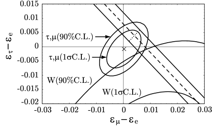
Figure 1: The experimentally allowed region of $(\epsilon_{\mu}-\epsilon_{e},\epsilon_{\tau}-\epsilon_{e})$ is shown. $\tau,\mu$ denote the constraints obtained from $\tau$ $\mu$ leptonic decays. $W$ denotes the bound obtained from $W\to l_{i}\bar{\nu}$ decays. The invisible decay width constraints Eq.(36) is also shown for $\epsilon_{e}=0$. The dotted line coresponds to the prediction of class B model (NH) case. (See section IV in text.)

The Inami-Lim function $\bar{E}(\frac{M_{I}^{2}}{m_{W}^{2}})$ is shown in Fig. 2.

Figure 2: Inami-Lim fiunctions $-\bar{E}$ (thick solid line) and $10\times F_{2}$ (dashed line) as functions of the singlet neutrino mass $M_{N}$ (GeV).

The typical values for the Inami-Lim function are $|{\bar{E}}|\sim 2.8\sim 8.1\ {\rm for}\ M=200\sim 2000~{}({\rm GeV})$. Finally, from the fact that the factor $u_{hI}u_{lI}^{\ast}$ depends on the flavor structure of $m_{D}$, the following relation

$$2|u_{hI}u_{lI}|\leq|u_{hI}|^{2}+|u_{lI}|^{2}\leq\sum_{i=e,\mu,\tau}|u_{iI}|^{2}=1,$$ (37)

leads us to the constraint, $|u_{hI}u_{lI}|^{2}\leq 0.25$. Then, numerical value of $S(h,l)$ for the case with $N$ degenerate $M_{i}$ and $X_{i}$ is

$$|S(h,l)|^{2}\leq\left(N\frac{X}{M}\right)^{2}\bar{E}\left(\frac{M^{2}}{M_{W}^{2}}\right)^{2}0.25\simeq 2\times 10^{-4}\ \sim 2\times 10^{-3},$$ (38)

where we denote $M_{i}\equiv M(i=1\sim N)$ and $X_{i}\sim X(i=1\sim N)$. The upper bound of the branching fractions for $b\to sl_{h}^{\mp}l_{l}^{\pm}$ is roughly predicted to be $10^{-11}\sim 10^{-10}$ for $200~{}({\rm GeV})<M<2000~{}({\rm GeV})$.

III Leptonic FCNC and QLFV rare decays with low mass scale singlet Majorana neutrinos

We now predict the branching fractions of the QLFV processes more concretely. As previously discussed, the branching fractions can be enhanced for rather large values of $X_{I}/M_{I}$. The large values of $X_{I}/M_{I}$ are realized for low scale of $M_{I}$, which may not generally be consistent with neutrino data. The large values of $X_{I}/M_{I}$ can be consistent with neutrino data when the contributions of $X_{I}$ to $m_{eff}$ in Eq. (19) are cancelled. Such a cancellation can be achieved by taking two almost degenerate small $M_{1,2}$ and tuning the relative phase between ${\bf u_{1}}$ and ${\bf u_{2}}$ so that those two terms contribute to $m_{eff}$ destructively while keeping $X_{3}$ so small that its contribution to $m_{eff}$ is suppressed. Thus, we need some specific flavor structure of Yukawa-Dirac mass term in order to obtain an enhancement of the branching fractions. Let us assume $X_{1}\sim X_{2}\gg X_{3}$ so as for $X_{12}\equiv X_{1}-X_{2}$ and $X_{3}$ to be of order the light neutrino mass squared differences $\sqrt{\Delta m_{\rm sol}^{2}}$ or $\sqrt{\Delta m_{\rm atm}^{2}}$. The relative phase of Yukawa-Dirac mass term from two singlet neutrinos $N_{1}$ and $N_{2}$ is tuned as ${\bf u_{2}}=i{\bf u_{1}}$. Then, $m_{eff}$ becomes

$$m_{eff}=-\left({\bf u_{1}}{\bf u_{1}^{T}}X_{12}+{\bf u_{3}}{\bf u_{3}^{T}}X_{3}\right).$$ (39)

We further assume the orthogonality of ${\bf u_{1}}$ and ${\bf u_{3}}$, $i.e.$ ${\bf u_{1}^{\dagger}\cdot u_{3}}=0$, so that ${\bf u_{1}}$ and ${\bf u_{3}}$ can be directly related to MNS matrix. Then, there exists a massless state due to the alignment of ${\bf u_{1}}$ and ${\bf u_{2}}$, which is assigned to $n_{1}=0$ for normal hierarchy and $n_{3}=0$ for inverted hierarchy. The other two masses are given by $X_{3}$ or $|X_{12}|$.

In Table 1, we classify the assignment of mass spectrum $(n_{1},n_{2},n_{3})$ and the unitary part of the mixing matrix $V_{0}$,

	$(n_{1},n_{2},n_{3})$	$V_{0}=({\bf v_{1},v_{2},v_{3}})$	flavor dependence of $b\to sl_{h}^{-}l_{l}^{+}$
Normal	$(0\sqrt{\Delta m_{\rm sol}^{2}},\sqrt{\Delta m_{\rm atm}^{2}+\Delta m_{\rm sol}^{2}})$
Class A	$(0,|X_{12}|,X_{3})$	$\left({\bf u_{1}^{\ast}\times u_{3}^{\ast}},{\bf u_{1}},{\bf u_{3}}\right)p$	${\bf v_{h2}v_{l2}^{\ast}}$
Class B	$(0,X_{3},|X_{12}|)$	$\left({\bf u_{1}^{\ast}\times u_{3}^{\ast}},{\bf u_{3}},{\bf u_{1}}\right)p$	${\bf v_{h3}v_{l3}^{\ast}}$
Inverted	$(\sqrt{\Delta m_{\rm atm}^{2}-\Delta m_{\rm sol}^{2}},\sqrt{\Delta m_{\rm atm}^{2}},0)$
Class A	$(|X_{12}|,X_{3},0)$	$\left({\bf u_{1}},{\bf u_{3}},{\bf u_{1}^{\ast}\times u_{3}^{\ast}}\right)p$	${\bf v_{h1}v_{l1}^{\ast}}$
Class B	$(X_{3},|X_{12}|,0)$	$\left({\bf u_{3}},{\bf u_{1}},{\bf u_{1}^{\ast}\times u_{3}^{\ast}}\right)p$	${\bf v_{h2}v_{l2}^{\ast}}$

Table 1: The assignment of mass spectrum and MNS matrix.

where $p$ is a diagonal Majorana phase which is irrelevant to the QFLV and LFV processes and thus we omit it from now on. Notice that $V_{0}$ is identical to the MNS matrix if we neglect its deviation from $V_{\rm MNS}$, $V_{0}-V_{\rm MNS}={\cal O}(\frac{m_{D}^{2}}{M^{2}})$. In fact, since the QLFV and LFV processes are already in the order of $\frac{{m_{D}}^{2}}{M^{2}}$ at the leading order, the difference can be safely ignored. The flavor dependence of the amplitudes for the QFLV and LFV processes is then extracted in terms of the mixing angles of the neutrino oscillation from $V_{0}=V_{\rm MNS}$:

$$V_{0} =\left(\begin{array}[]{ccc}c_{13}c_{\rm sol}&c_{13}s_{\rm sol}&0\\ -s_{\rm sol}c_{\rm atm}&c_{\rm atm}c_{\rm sol}&c_{13}s_{\rm atm}\\ s_{\rm sol}s_{\rm atm}&-s_{\rm atm}c_{\rm sol}&c_{13}c_{\rm atm}\end{array}\right)+s_{13}\left(\begin{array}[]{ccc}0&0&\exp(-i\delta)\\ -c_{\rm sol}s_{\rm atm}\exp(i\delta)&-s_{\rm sol}s_{\rm atm}\exp(i\delta)&0\\ -c_{\rm sol}c_{\rm atm}\exp(i\delta)&-s_{\rm sol}c_{\rm atm}\exp(i\delta)&0\end{array}\right),$$ (46)

where we take $s_{\rm sol}=0.56,~{}~{}c_{\rm sol}=0.84$ and $s_{\rm atm}=c_{\rm atm}=\sqrt{\frac{1}{2}}$.

In Table 2, we present the relevant combinations of ${\bf v}_{ij}$ which correspond to the flavor dependence shown in the fourth column of Table I. The value of $s_{13}$ is very small and thus we ignore the terms of order ${\cal O}(s^{2}_{13})$.

${{\bf v}}_{\mu 2}{\bf v}_{e2}^{\ast}$	$c_{13}s_{\rm sol}c_{\rm sol}c_{\rm atm}$	$0.33c_{13}$
${\bf v}_{\tau 2}{\bf v}_{\mu 2}^{\ast}$	$-c_{\rm atm}s_{\rm atm}c_{\rm sol}^{2}$	$-0.35$
${\bf v}_{\tau 2}{\bf v}_{e2}$	$-c_{13}s_{\rm atm}c_{\rm sol}s_{\rm sol}$	$-0.33c_{13}$
${\bf v}_{\mu 3}{\bf v}_{e3}^{\ast}$	$c_{13}s_{\rm atm}s_{13}\exp(i\delta)$	$0.71s_{13}c_{13}\exp(i\delta)$
${\bf v}_{\tau 3}{\bf v}_{\mu 3}^{\ast}$	$c_{13}^{2}s_{\rm atm}c_{\rm atm}$	$0.5c_{13}^{2}$
${\bf v}_{\tau 3}{\bf v}_{e3}$	$c_{13}c_{\rm atm}s_{13}\exp(i\delta)$	$0.71s_{13}c_{13}\exp(i\delta)$
${\bf v}_{\mu 1}{\bf v}_{e1}^{\ast}$	$-c_{13}c_{\rm sol}s_{\rm sol}c_{\rm atm}$	$-0.33c_{13}$
${\bf v}_{\tau 1}{\bf v}_{\mu 1}^{\ast}$	$-s_{\rm sol}^{2}c_{\rm atm}s_{\rm atm}$	$-0.16$
${\bf v}_{\tau 1}{\bf v}_{e1}^{\ast}$	$c_{13}c_{\rm sol}s_{\rm sol}s_{\rm atm}$	$0.33c_{13}$

Table 2: The combinations of ${\bf v}_{ij}$ relevant to the flavor dependence of QLFV and LFV decays.

Then, the suppression factor $S(h,l)$ is approximately given by

$$S(h,l) \simeq \left(\frac{X}{M_{1}}\bar{E}(x_{t},x_{c},y_{1})+\frac{X}{M_{2}}\bar{E}(x_{t},x_{c},y_{2})\right){\bf v_{h\alpha}}{\bf v_{l\alpha}^{\ast}},$$ (48)

where $\alpha$ denotes the index depending on the class and neutrino mass hierarchy, $X_{1}\simeq X_{2}\equiv X$. And the term proportional to $\frac{X_{3}}{M_{3}}$ is not relevant at all and thus ignored. By using Eq. (48), the ratios of the branching fractions are given by

$$\frac{{\rm Br}(b\to s\tau^{\pm}e^{\mp})}{{\rm Br}(b\to s\tau^{\pm}\mu^{\mp})}=\left|\frac{{\bf v}_{\tau\alpha}{\bf v}^{\ast}_{e\alpha}}{{\bf v}_{\tau\alpha}{\bf v}^{\ast}_{\mu\alpha}}\right|^{2},$$ (49)

$$\frac{{\rm Br}(b\to s\mu^{\pm}e^{\mp})}{{\rm Br}(b\to s\tau^{\pm}\mu^{\mp})}=\frac{P(\frac{m_{\mu}}{m_{b}})}{P(\frac{m_{\tau}}{m_{b}})}\left|\frac{{\bf v}_{\mu\alpha}{\bf v}^{\ast}_{e\alpha}}{{\bf v}_{\tau\alpha}{\bf v}^{\ast}_{\mu\alpha}}\right|^{2},$$ (50)

where $P(\frac{m_{\mu}}{m_{b}})$, and $P(\frac{m_{\tau}}{m_{b}})$ are phase space factors and $\frac{P(\frac{m_{\mu}}{m_{b}})}{P(\frac{m_{\tau}}{m_{b}})}=2.74$.

In Table III, the numerical results of the ratios of the branching fractions given in Eqs. (49,50) are presented.

	Class A NH (Class B IH)	Class B NH	Class A IH
$\frac{{\rm Br}(b\to s\tau^{\pm}e^{\mp})}{{\rm Br}(b\to s\tau^{\pm}\mu^{\mp})}$	$\left(\frac{s_{\rm atm}c_{\rm sol}s_{\rm sol}}{c_{\rm atm}s_{\rm atm}c_{\rm sol}^{2}}\right)^{2}=0.89$	$\left(\frac{c_{\rm atm}s_{13}}{s_{\rm atm}c_{\rm atm}}\right)^{2}=2.0s^{2}_{13}$	$\left(\frac{c_{\rm sol}s_{\rm sol}s_{\rm atm}}{s_{\rm sol}^{2}c_{\rm atm}s_{\rm atm}}\right)^{2}=4.5$
$\frac{{\rm Br}(b\to s\mu^{\pm}e^{\mp})}{{\rm Br}(b\to s\tau^{\pm}\mu^{\mp})}$	$\left(\frac{s_{\rm sol}c_{\rm sol}c_{\rm atm}}{c_{\rm atm}s_{\rm atm}c_{\rm sol}^{2}}\right)^{2}\frac{P_{\mu}}{P_{\tau}}=2.4$	$\left(\frac{s_{\rm atm}s_{13}}{s_{\rm atm}c_{\rm atm}}\right)^{2}\frac{P_{\mu}}{P_{\tau}}=5.5s^{2}_{13}$	$\left(\frac{c_{\rm sol}s_{\rm sol}c_{\rm atm}}{s_{\rm sol}^{2}c_{\rm atm}s_{\rm atm}}\right)^{2}\frac{P_{\mu}}{P_{\tau}}=12.0$

Table 3: Ratios of the branching fractions of $b\to sl_{h}^{-}l_{l}^{+}$. $P_{\mu}\equiv P(\frac{m_{\mu}}{m_{b}})$ and $P_{\tau}\equiv P(\frac{m_{\tau}}{m_{b}})$.

	Class A NH (Class B IH)	Class B NH	Class A IH
$\frac{{\rm Br}(\tau\to e\gamma)}{{\rm Br}(\tau\to\mu\gamma)}$	$\left(\frac{s_{\rm atm}c_{\rm sol}s_{\rm sol}}{c_{\rm atm}s_{\rm atm}c_{\rm sol}^{2}}\right)^{2}=0.89$	$\left(\frac{c_{\rm atm}s_{13}}{s_{\rm atm}c_{\rm atm}}\right)^{2}=2.0s_{13}^{2}$	$\left(\frac{c_{\rm sol}s_{\rm sol}s_{\rm atm}}{s_{\rm sol}^{2}c_{\rm atm}s_{\rm atm}}\right)^{2}=4.5$
$\frac{{\rm Br}(\mu\to e\gamma)}{{\rm Br}(\tau\to\mu\gamma)}$	$\left(\frac{s_{\rm sol}c_{\rm sol}c_{\rm atm}}{c_{\rm atm}s_{\rm atm}c_{sol}^{2}}\right)^{2}\frac{\tau_{\mu}}{\tau_{\tau}}\left(\frac{m_{\mu}}{m_{\tau}}\right)^{5}=5.0$	$\left(\frac{s_{\rm atm}s_{13}}{s_{\rm atm}c_{\rm atm}}\right)^{2}\frac{\tau_{\mu}}{\tau_{\tau}}\left(\frac{m_{\mu}}{m_{\tau}}\right)^{5}=11s_{13}^{2}$	$\left(\frac{c_{\rm sol}s_{\rm sol}c_{\rm atm}}{s_{\rm sol}^{2}c_{\rm atm}s_{\rm atm}}\right)^{2}\frac{\tau_{\mu}}{\tau_{\tau}}\left(\frac{m_{\mu}}{m_{\tau}}\right)^{5}=25$

Table 4: Ratios of the branching fractions of $l_{h}\to l_{l}\gamma$.

It can be seen that in Class B model for NH case, only $b\to s\tau^{-}\mu^{+}$ can be much larger than the other channel because of the absence of the suppression factor $s_{13}^{2}$ for $\tau\mu$ final states, while the branching fractions of the different channels in models except Class B for NH case are within a factor of 10. Furthermore, as discussed in Ref. [14], there is strong correlation between QLFV processes and LFV radiative decays $l_{h}\to l_{l}\gamma$. Experimentally, there are stringent bounds as ${\rm Br}(\mu\to e\gamma)<1.2\times 10^{-11}$ [30], ${\rm Br}(\tau\to\mu\gamma)<6.8\times 10^{-8}$ [31] and ${\rm Br}(\tau\to e\gamma)<1.1\times 10^{-7}(3.9\times 10^{-7})$ [32, 33]. The bounds on the LFV processes stringently constrain the branching fractions for QLFV processes.

We note that the bound on $\frac{X}{M}$ from the invisible decay width of $Z$ and the present upper bound on $\mu\to e\gamma$ are not compatible with each other for Class A and Class B IH case, as shown in Table IV. The branching fraction for $l_{h}\to l_{l}\gamma$ is,

$${\rm Br}(l_{h}\to l_{l}\gamma)=\frac{\alpha^{3}}{256\pi^{2}s_{W}^{4}}\frac{m_{h}^{4}}{M_{W}^{4}}\frac{m_{h}}{\Gamma_{h}}|G|^{2}.$$ (51)

Numerically computing the pre-factors, the branching fractions are given by

$${\rm Br}(\tau\to\mu\gamma) = 5.4\times 10^{-4}|G(\tau,\mu)|^{2},$$

$${\rm Br}(\tau\to e\gamma) = 5.4\times 10^{-4}|G(\tau,e)|^{2},$$

$${\rm Br}(\mu\to e\gamma) = 3.1\times 10^{-3}|G(\mu,e)|^{2},$$ (52)

where $G$ is a suppression factor defined by

$$G = \sum_{\alpha=4}^{3+N}V_{l\alpha}V_{h\alpha}^{\ast}F_{2}(y_{\alpha})$$ (53)

$$= \sum_{I=1}^{N}u_{lI}u_{hI}^{\ast}\frac{X_{I}}{M_{I}}F_{2}(y_{I}),$$

where $y_{I}=\frac{M_{I}^{2}}{m_{W}^{2}}$ and $F_{2}$ is Inami-Lim function, $F_{2}(y)=-\frac{2y^{3}+5y^{2}-y}{4(1-y)^{3}}-\frac{3y^{3}\log y}{2(y-1)^{4}}$, as shown in Fig. 2.

With $M_{1}=M_{2}=M\ll M_{3}$ and $X_{1}\simeq X_{2}=X\gg X_{3}$, for Class A and Class B (IH) model, we predict,

$${\rm Br}(\mu\to e\gamma)=3.1\times 10^{-3}\left(\frac{2X}{M}\right)^{2}(0.33)^{2}F_{2}(y)^{2}\geq 4.4\times 10^{-10},$$ (54)

where we have used $\frac{2X}{M}\geq 0.004$ and $M\geq 200$ (GeV). Therefore, Class A and Class B (IH) models are excluded. If the bound on $\frac{X}{M}$ in Eq. (32) is not taken into account, one can obtain from Eqs. (27,52),

$${\rm Br}(b\to s\tau^{-}\mu^{+}) = 1.9\times 10^{-4}{\rm Br}(\tau\to\mu\gamma)\frac{|S(\tau\mu)|^{2}}{|G(\tau\mu)|^{2}}\leq 1.3\times 10^{-11}\left|\frac{S(\tau\mu)}{G(\tau\mu)}\right|^{2},$$

$${\rm Br}(b\to s\tau^{-}e^{+}) = 1.9\times 10^{-4}{\rm Br}(\tau\to e\gamma)\frac{|S(\tau e)|^{2}}{|G(\tau e)|^{2}}\leq 2.0\times 10^{-11}\left|\frac{S(\tau e)}{G(\tau e)}\right|^{2},$$

$${\rm Br}(b\to s\mu^{-}e^{+}) = 9.0\times 10^{-5}{\rm Br}(\mu\to e\gamma)\frac{|S(\mu e)|^{2}}{|G(\mu e)|^{2}}\leq 1.1\times 10^{-15}\left|\frac{S(\mu e)}{G(\mu e)}\right|^{2}.$$ (55)

While Eq. (55) depends neither on the mass spectrum of heavy Majorana neutrinos nor on the flavor structure of Yukawa-Dirac mass terms, the ratio of $|\frac{S}{G}|$ depends on the details of them. For the present case with $M_{1}=M_{2}=M\ll M_{3}$ and $X_{1}=X_{2}=X\gg X_{3}$, the ratio $|S(h,l)/G(h,l)|$ is simply given as,

$$\left|\frac{S(h,l)}{G(h,l)}\right|^{2}=\left|\frac{\bar{E}(x_{t},x_{c},y)}{F_{2}(y)}\right|^{2}=98~{}(M=200~{}{\rm GeV})\sim 285~{}(M=2000~{}{\rm GeV}).$$ (56)

Therefore, the upper bounds on the branching fractions given in Eq. (55) are translated to

$${\rm Br}(b\to s\tau^{-}e^{+}) \leq(1.3\sim 3.6)\times 10^{-9}$$

$${\rm Br}(b\to s\tau^{-}\mu^{+}) \leq(2.0\sim 5.0)\times 10^{-9}$$

$${\rm Br}(b\to s\mu^{-}e^{+}) \leq(1.1\sim 3.0)\times 10^{-13}.$$ (57)

The range of the upper bounds corresponds to $M=200\sim 2000$ (GeV). For Class A and Class B with IH case, by combining $\mu\to e\gamma$ upper limit, we may obtain much tighter bound on the other LFV and QLFV processes. Let us consider Class A (NH) and Class B (IH) cases. From Table 3 and Table 4, the upper bounds on ${\rm Br}(\mu\to e\gamma)$ and ${\rm Br}(b\to s\mu^{-}e^{+})$ obtained in Eq. (57) severely constrain the other modes,

$${\rm Br}(b\to s\tau^{-}e^{+}) \leq(0.41\sim 1.1)\times 10^{-13},$$

$${\rm Br}(b\to s\tau^{-}\mu^{+}) \leq(0.46\sim 1.25)\times 10^{-13},$$

$${\rm Br}(\tau\to\mu\gamma) \leq 2.4\times 10^{-12},$$

$${\rm Br}(\tau\to e\gamma) \leq 2.1\times 10^{-12}.$$ (58)

The bounds similar to Eq. (58) are obtained for Class A IH case,

$${\rm Br}(b\to s\tau^{-}e^{+}) \leq(0.41\sim 1.1)\times 10^{-13},$$

$${\rm Br}(b\to s\tau^{-}\mu^{+}) \leq(0.92\sim 2.5)\times 10^{-14},$$

$${\rm Br}(\tau\to\mu\gamma) \leq 4.8\times 10^{-13},$$

$${\rm Br}(\tau\to e\gamma) \leq 2.2\times 10^{-12}.$$ (59)

We note that the upper bound of the branching fractions of QLFV processes for Class A (NH, IH) and Class B (IH) models are $10^{-14}\sim 10^{-13}$ and the branching fractions for LFV processes is $10^{-13}\sim 10^{-12}$. As we have already shown in Eq.(54), the Class A model and Class B model for IH case can not satisfy the upper limit of the branching fraction of $\mu\to e\gamma$ and constraint from the effective light neutrinos number $N_{\nu}$ simultaneously. This is because the former requires very small $\frac{X}{M}$, while the latter requires larger $\frac{X}{M}$. Below, we show Class B model for NH case may satisfy both constraints. Furthermore, the model predicts the large branching fractions of $\tau\to\mu\gamma$ and $b\to s\tau\mu$ which are within the reach of near future Super $B$ factories [34, 35]. If we take into account the constraints coming from ${\rm Br}(\mu\to e\gamma)$ and the effective number of light neutrinos $N_{\nu}$, we can have the parameter regions consistent with the present bounds only for Class B model with NH case. In this class, the stringent experimental limit on ${\rm Br}(\mu\to e\gamma)$ is not effective on ${\rm Br}(\tau\to\mu\gamma)$ and ${\rm Br}(b\to s\tau\mu)$, because the former process is proportional to $s_{13}^{2}$ and thus ignorable, but the latter processes are not suppressed by the factor.

In Fig. 3, we have shown the correlation of branching fractions between $\mu\to e\gamma$ and the other LFV and QLFV processes in Class B model for NH case.

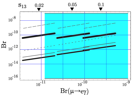
Figure 3: Correlation between the branching fraction for $\mu\to e\gamma$ and the branching fractions for $b\to s\tau\mu$ (thick solid line) $b\to s\tau e$ (solid line) $b\to s\mu e$ (thin solid line), $\tau\to\mu\gamma$ (long dashed line) $\tau\to e\gamma$ (dashed line) for Class B model with NH case. From left to right, the lines correspond to $s_{13}=0.02,0.05,0.1$, repectively. The shaded region is excluded by the current bound on $Br(\mu\to e\gamma)$.

The numerical results in Fig. 3 are obtained as follows: We first set $X_{1}\sim X_{2}=X$ and $M_{2}=M_{1}=M$. From the constraint given in Eq. (32), the allowed range of $M$ is ,

$$\frac{m_{D1}}{\sqrt{\sigma_{\rm max}}}\sqrt{2}<M<\frac{m_{D1}}{\sqrt{\sigma_{\rm min}}}\sqrt{2},$$ (60)

with $\sigma_{\rm min}=0.004,\sigma_{\rm max}=0.012$. When we fix $m_{D1}$, the allowed range of $M$ is determined. By varying $M$ within the above range, we plot the correlation between ${\rm Br}(\mu\to e\gamma)$ and the other five QLFV and LFV branching fractions. Here, $s_{13}$ is a free parameter and is chosen to be $0.02,0.05$ and $0.1$. $m_{D1}$ is chosen to be $100$ (GeV). As can be seen in Fig. 3, the present upper limit on ${\rm Br}(\mu\to e\gamma)$ gives a very tight bound on $s_{13}$, typically smaller than $0.02$. With this small $s_{13}$, $\tau\to e\gamma$ and $b\to s\tau(\mu)e$ are also severely suppressed. Only $b\to s\tau\mu$ and $\tau\to\mu\gamma$ are free from the suppression and the former branching fraction can be as large as $10^{-10}$ and the latter can be $10^{-9}$. They are independent on small $s_{13}$.

We show in Fig. 4 and Fig. 5 the dependence of the branching fractions of $b\to s\tau\mu$ and $\tau\to\mu\gamma$ on $m_{D1}$ and the heavy Majorana neutrino mass for the exact degenerate case, $i.e.$ $M_{1}=M_{2}=M$. We fix $m_{D1}$ to $20,50,100,200$ (GeV). Although the branching fractions become small as $m_{D1}$ becomes small, the change of the branching fractions is within a factor 10.

Figure 4: ${\rm Br}(b\to s\tau\mu)$ vs. $M$ for Class B (NH). From left to right, the curves correspond to $m_{D1}=20,50,100,200$ (GeV), respectively.

Figure 5: ${\rm Br}(\tau\to\mu\gamma)$ vs. $M$ for Class B (NH). From left to right, the curves correspond to $m_{D1}=20,50,100,200$ (GeV),respectively.

We also consider the non-degenerate case for Majorana neutrino masses ($M_{1}\equiv M\neq M_{2}$) while keeping the degeneracy $X_{1}\sim X_{2}=X$. By setting $M_{2}\equiv RM_{1}$ and $M_{1}\equiv M$, the dependence of the branching fraction $b\to s\tau\mu$ on the ratio $R$ is studied. The allowed range of the lightest heavy Majorana neutrino mass $M$ of Eq. (60) is modified as $\frac{m_{D1}}{\sqrt{\sigma_{\rm max}}}\sqrt{1+\frac{1}{R}}<M<\frac{m_{D1}}{\sqrt{\sigma_{\rm min}}}\sqrt{1+\frac{1}{R}}$. From Fig. 6, we find that the lower and the upper limits of $M$ become smaller as $R$ becomes larger. However, the branching fraction does not change so significantly.

Figure 6: ${\rm Br}(b\to s\tau\mu)$ vs. $M$ for Class B (NH). We fix $m_{D1}=100$ (GeV). From right to left, the curves correspond to the ratio $R=\frac{M_{2}}{M}$ $1,2,10$, respectively.

IV summary and discussion

As shown, the contributions of the singlet Majorana neutrinos to QLFV and LFV decays can be significant in the low scale seesaw model motivated by resonant leptogenesis. The branching fractions of inclusive decays $b\to sl_{h}^{\pm}l_{l}^{\mp}$ in the seesaw model considered in this paper depends on the suppression factor $\frac{m_{D}}{M}$ which is arisen from the mixing between the singlet heavy neutrinos with three light neutrinos, and can be as large as about $10\%$ without being in conflict with the neutrino mass squared differences from neutrino data and the current bound on the invisible decay width of $Z$ boson.

We have classified four classes of the model along with the light neutrino mass spectrum and the assignment of the mixing matrix $V_{0}$, and studied how the ratios of the branching fractions for the various channels of QLFV and LFV decays along with lepton flavors could be distinctively predicted in each class. We have found that only the class B for NH case presented in Table I survives the current limit on $Br(\mu\to e\gamma)$ and the invisible decay width of Z boson. One may check if the model is consistent with the experiments of lepton universality tests. The class B for NH case predicts

$$\epsilon_{e} = \frac{2X}{M}s_{13}^{2}\leq 5\times 10^{-6}\ (s_{13}\leq 0.02),$$

$$\epsilon_{\mu} = \frac{2X}{M}s_{\rm atm}^{2}c_{13}^{2}\simeq 0.004,$$

$$\epsilon_{\tau} = \frac{2X}{M}c_{\rm atm}^{2}c_{13}^{2}\simeq 0.004.$$ (61)

The model predicts very small $\epsilon_{e}$ and $\epsilon_{\mu}=\epsilon_{\tau}$ which are shown in Fig.(1) with dotted line. The model is consistent with the constraint of Z invisible decay width and the lepton universalty constraints from $\tau$ and $\mu$ decays while it may not be consistent with the lepton universality constraints determined by $W$ decays. In this class, the branching fractions of $b\to s\tau\mu$ and $\tau\to\mu\gamma$ are predicted to be as large as $10^{-10}$ and $10^{-9}$, respectively. Such large branching fractions can be tested in the future $B$ factory experiments. The enhancment of the branching fractions of QFLV and LFV is originated from the one loop Feynman diagrams in which the heavy Majorana neutrinos contribute to and it is non-susy contribution.

Acknowledgements

We thank K. Homma and K. Ishikawa for useful discussions. C.S.K. was supported in part by JSPS, in part by CHEP-SRC Program, in part by the Korea Research Foundation Grant funded by the Korean Government (MOEHRD) No. R02-2003-000-10050-0 and in part by No. KRF-2005-070-C00030. T.M. is supported by the kakenhi of MEXT, Japan, No. 16028213. S.K.K. was supported in part by BK21 program of the Ministry of Education in Korea.

References

• [1] P. Minkowski, Phys. Lett. B67, 421 (1977).
• [2] T. Yanagida, in the proceedings of the Workshop on Unified Theories and Baryon Number in the Universe, edited by O. Sawada and A. Sugamoto, 95 (1979).
• [3] M. Gell-Mann, P. Ramond and R. Slansky, in Supergravity, P. van Nieuwenhuizen and D.Z. Freedman (eds.), North Holland Publ. Co.,(1979).
• [4] R. N. Mohapatra and G. Senjanovich, Phys. Rev. Lett. 44, 912 (1980).
• [5] M. Fukugita and T. Yanagida, Phys. Lett. B174, 45 (1986).
• [6] A. Pilaftsis, Int. J. Mod. Phys. A14, 1811 (1999).
• [7] A. Pilaftsis and T. E. J. Underwood, Nucl. Phys. B692, 303 (2004).
• [8] R. Gonzalez Felipe, F. R. Joaquim, and B. M. Nobre, Phys. Rev. D70, 085009 (2004).
• [9] G.C. Branco, R. Gonzalez Felipe, F. R. Joaquim and B. M. Nobre, [Archive:hep-ph/0507092].
• [10] M. Raidal, A. Strumia, and K. Turzynski, Phys. Lett. B609, 351 (2005), [Archive:hep-ph/0408015].
• [11] S. M. West, Phys. Rev. D71, 013004 (2005), [Archive: hep-ph/0408318].
• [12] T. Hambye, J. March-Russell, S. M. West, JHEP 0407, 070 (2004), [Archive:hep-ph/0403183].
• [13] J. March-Russell, S. M. West, Phys. Lett. B593, 181 (2004), [Archive:hep-ph/0403067].
• [14] Xiao-Gang He, G. Valencia and Yili Wang, Phys. Rev. D70, 113011 (2004).
• [15] Belle Collaboration: A. Ishikawa $et~{}al.$, Phys. Rev. Lett. 91, 261601 (2003).
• [16] B. W. Lee, S.Pakvasa, R.E. Shrock and H. Sugawara, Phys. Rev. Lett. 38, 937 (1977).
• [17] T. Inami and C. S. Lim, Prog. Theor. Phys. 67, 1569 (1982).
• [18] G. Cvetic, C. O. Dib, C. S. Kim and J. D. Kim, Phys. Rev. D 71, 113013 (2005) [arXiv:hep-ph/0504126]; G. Cvetic, C. Dib, C. S. Kim and J. D. Kim, Phys. Rev. D 66, 034008 (2002) [Erratum-ibid. D 68, 059901 (2003)] [arXiv:hep-ph/0202212].
• [19] A. Pilaftsis, Phys. Rev. Lett. 95, 081602 (2005).
• [20] A. Pilaftsis and T.E.J. Underwood, [arXiv:hep-ph/0506107].
• [21] G. C. Branco, T. Morozumi, B. Nobre and M. N. Rebelo, Nucl. Phys. B617, 475 (2001).
• [22] A. Broncano, M. B. Gavela and E. Jenkins, Nucl. Phys. B672, 163 (2003).
• [23] T. Fujihara, S. Kaneko, S. Kang, D. Kimura, T. Morozumi and M. Tanimoto, Phys. Rev. D 72, 016006 (2005) [arXiv:hep-ph/0505076].
• [24] T. Inami and C. S. Lim, Prog. Theor. Phys. 65, 297 (1981); 65,1772(E)(1981).
• [25] Z. Gagyi-Palffy, A. Pilaftsis and K. Schilcher, Phys. Lett. B343, 275 (1995).
• [26] Will Loinaz, N. Okamura, S. Rayyan and T. Takeuchi, Phys. Rev. D68, 073001 (2003).
• [27] S. L. Glashow, [arXiv:hep-ph/0301250].
• [28] Will Loinaz, N. Okamura, S. Rayyan and T. Takeuchi Phys. Rev. D70, 113004 (2004).
• [29] The LEP Collaborations ALEPH, DELPHI, L3, OPAL, the LEP Electroweak Working Group, the SLD Electroweak and Heavy Flavor Groups, [arXiv:hep-ex/0312023].
• [30] MEGA Collaboration: M. L. Brooks et al., Phys. Rev. Lett. 83, 1521 (1999); MEGA Collaboration: M. Ahmed et al., Phys. Rev. D65, 112002 (2002).
• [31] BABAR Collaboration: B. Aubert et al., Phys. Rev. Lett. 95, 041802 (2005).
• [32] BABAR Collaboration: B. Aubert et al., [arXiv:hep-ex/0508012].
• [33] Belle Collaboration: K. Hayasaka et al., Phys. Lett. B613, 20 (2005).
• [34] Physics at Super $B$ Factory, by SuperKEKB Physics Working Group, A. G. Akeroyd et al., [arXiv:hep-ex/0406071].
• [35] The Discovery Potential of a Super $B$ Factory. Proceedings, SLAC Workshops, Stanford, USA (2003), J. Hewett, (ed.) et al., [arXiv:hep-ph/0503261].