Generalized Dual Symmetry of Nonabelian Theories and the Freezing of ${\Large\bf\alpha_{s}}$

Abstract

The quantum Yang–Mills theory, describing a system of fields with non–dual (chromo–electric $g$) and dual (chromo–magnetic $\tilde{g}$) charges and revealing the generalized dual symmetry, is developed by analogy with the Zwanziger formalism in QED. The renormalization group equations (RGEs) for pure nonabelian theories are analysed for both constants, $\alpha=g^{2}/4\pi$ and $\tilde{\alpha}={\tilde{g}}^{2}/4\pi$. The pure $SU(3)\times\widetilde{SU(3)}$ gauge theory is investigated as an example. We consider not only monopoles, but also dyons. The behaviour of the total $SU(3)$ $\beta$–function is investigated in the whole region of $\alpha\equiv\alpha_{s}$: $0\leq\alpha<\infty$. It is shown that this $\beta$–function is antisymmetric under the interchange $\alpha\leftrightarrow 1/\alpha$ and is given by the well–known perturbative expansion not only for $\alpha\ll 1$, but also for $\alpha\gg 1$. Using an idea of the Maximal Abelian Projection by t’ Hooft, we have considered the formation of strings – the ANO flux tubes – in the Higgs model of scalar monopole (or dyon) fields. In this model we have constructed the behaviour of the $\beta$–function in the vicinity of the point $\alpha=1$, where it acquires a zero value. Considering the phase transition points at $\alpha\approx 0.4$ and $\alpha\approx 2.5$, we give the explanation of the freezing of $\alpha_{s}$. The evolution of $\alpha_{s}^{-1}(\mu)$ with energy scale $\mu$ and the behaviour of $V_{eff}(\mu)$ are investigated for both, perturbative and non–perturbative regions of QCD. It was shown that the effective potential has a minimum, ensured by the dual sector of QCD. The gluon condensate $F^{2}_{0}$, corresponding to this minimum, is predicted: $F^{2}_{0}\approx 0.15$ GeV⁴, in agreement with the well–known results.

1 Introduction

In the last years gauge theories essentially operate with the fundamental idea of duality [1, 2, 3, 4, 5, 6, 7, 8, 9, 10, 11, 12, 13, 14, 15, 16, 17, 18, 19, 20, 21, 22].

Duality is a symmetry appearing in pure electrodynamics as invariance of the free Maxwell equations:

$${\bigtriangledown}\cdot\vec{\bf B}=0,\qquad{\bigtriangledown}\times\vec{\bf E}=-\partial_{0}\vec{\bf B},$$ (1)

$${\bigtriangledown}\cdot\vec{\bf E}=0,\qquad{\bigtriangledown}\times\vec{\bf B}=\partial_{0}\vec{\bf E},$$ (2)

under the interchange of electric and magnetic fields:

$$\vec{\bf E}\to\vec{\bf B},\qquad\vec{\bf B}\to-\vec{\bf E}.$$ (3)

Letting

$$F=\partial\wedge A=-(\partial\wedge B)^{*},$$ (4)

$$F^{*}=\partial\wedge B=(\partial\wedge A)^{*},$$ (5)

we see that the equations of motion:

$$\partial_{\lambda}F_{\lambda\mu}=0,$$ (6)

together with the Bianchi identity:

$$\partial_{\lambda}F_{\lambda\mu}^{*}=0,$$ (7)

are equivalent to Eqs. (1) and (2), and show the invariance under the Hodge star operation on the field tensor:

$$F_{\mu\nu}^{*}=\frac{1}{2}\epsilon_{\mu\nu\rho\sigma}F_{\rho\sigma}.$$ (8)

This Hodge star duality, having a long history [1, 2, 3, 4, 5, 6, 7, 8, 9, 10, 11, 12, 13, 14, 15, 16, 17, 18, 19, 20, 21], does not hold in general for nonabelian theories. In abelian theory Maxwell’s equation (6) is equivalent to the Bianchi identity for the dual field $F_{\mu\nu}^{*}$, which guarantees the existence of a dual potential $B_{\mu}$ given by Eq. (5).

In the nonabelian theory, one usually starts with a gauge field $F_{\mu\nu}(x)$ derivable from a potential $A_{\mu}(x)$:

$$F_{\mu\nu}=\partial_{\nu}A_{\mu}(x)-\partial_{\mu}A_{\nu}(x)+ig[A_{\mu}(x),A_{\nu}(x)].$$ (9)

Considering only gauge groups with the Lie algebra of $SU(N)$, we have:

$$A_{\mu}(x)=t^{j}A_{\mu}^{j}(x),\qquad j=1,...,N^{2}-1,$$ (10)

where $t^{j}$ are the generators of $SU(N)$ group. Equations of motion obtained by extremizing the corresponding action with respect to $A_{\mu}(x)$ gives:

$$D_{\nu}F^{\mu\nu}(x)=0,$$ (11)

where $D_{\mu}$ is the covariant derivative defined as

$$D_{\mu}=\partial_{\mu}-ig[A_{\mu}(x),...].$$ (12)

The analogy to electromagnetism is still rather close. But Yang–Mills equation (11) does not imply in general the existence of a potential for the corresponding dual field $F_{\mu\nu}^{*}$. This Yang–Mills equation itself can no longer be interpreted as the Bianchi identity for $F_{\mu\nu}^{*}(x)$, nor does it imply the existence of a dual potential ${\tilde{A}}_{\mu}(x)$ satisfying

$$F_{\mu\nu}^{*}(x)\stackrel{{\scriptstyle?}}{{=}}\partial_{\nu}{\tilde{A}}_{\mu}(x)-\partial_{\mu}{\tilde{A}}_{\nu}(x)+i{\tilde{g}}[{\tilde{A}}_{\mu}(x),{\tilde{A}}_{\nu}(x)],$$ (13)

in parallel to (9). This result means that the dual symmetry of the Yang–Mills theory under the Hodge star operation does not hold. So one has to seek a more general form of duality for nonabelian theories than the Hodge star operation on the field tensor.

It was shown in [14, 15, 16, 17, 18, 19] that the classical Yang–Mills theory i s symmetric under a generalized dual transform which reduces to the well–known electromagnetic duality of the abelian case.

2 Loop space variables of nonabelian theories

As in Refs. [14, 15, 16, 17, 18, 19, 20, 21], we investigate the $SU(N)$ nonabelian theories in terms of loop variables. For usual (non–dual) sector we consider the path ordered exponentials with closed loops (see Fig. 1):

$$\Phi(C)=P\exp\left[ig\oint_{C}A_{\mu}(\xi)d{\xi}^{\mu}\right]=P\exp\left[ig\int_{0}^{2\pi}A_{\mu}(\xi)\dot{\xi}^{\mu}(s)ds\right],$$ (14)

where $C$ is a parameterized closed loop with coordinates ${\xi}^{\mu}(s)$ in the 4–dimensional space. The loop is parameterized by $s$: $0\leq s\leq 2\pi$, and

$$\dot{\xi}^{\mu}(s)=\frac{d{\xi}^{\mu}(s)}{ds}.$$ (15)

We also consider the following unclosed loop variable [23]:

$$\Phi(s_{1},s_{2})=P\exp\left[ig\int_{s_{1}}^{s_{2}}A_{\mu}(\xi)\dot{\xi}^{\mu}(s)ds\right].$$ (16)

Therefore, $\Phi(C)\equiv\Phi(0,2\pi)$.

For the dual sector we have (see Fig. 2):

$$\tilde{\Phi}(\tilde{C})=P\exp\left[i\tilde{g}\oint_{\tilde{C}}{\tilde{A}}_{\mu}(\eta)d{\eta}^{\mu}\right]=P\exp\left[i\tilde{g}\int_{0}^{2\pi}{\tilde{A}}_{\mu}(\eta)\dot{\eta}^{\mu}(t)dt\right],$$ (17)

where $\tilde{C}$ is a parameterized closed loop in the dual sector with coordinates $\eta^{\mu}(t)$ in the 4–dimensional space, and the loop parameter is $t$: $0\leq t\leq 2\pi$;

$$\dot{\eta}^{\mu}(t)=\frac{d\eta^{\mu}(t)}{dt}.$$ (18)

The unclosed loop variables in the dual sector are:

$$\tilde{\Phi}(t_{1},t_{2})=P\exp\left[i\tilde{g}\int_{t_{1}}^{t_{2}}\tilde{A}_{\mu}(\eta)\dot{\eta}^{\mu}(t)dt\right].$$ (19)

Therefore, $\tilde{\Phi}(\tilde{C})\equiv\tilde{\Phi}(0,2\pi)$. Here standard and dual sectors have coupling constants $g$ and $\tilde{g}$ respectively.

Considering (for simplicity of presentation) only gauge groups $SU(N)$, we have vector–potentials $A_{\mu}$ and $\tilde{A}_{\mu}$ belonging to the adjoint representation of $SU(N)$ and $\widetilde{SU(N)}$ groups:

$$A_{\mu}(x)=t^{j}A_{\mu}^{j},\qquad\tilde{A}_{\mu}(x)=t^{j}\tilde{A}_{\mu}^{j},\qquad j=1,...,N^{2}-1.$$ (20)

As a result, we consider nonabelian theories having a doubling of symmetry from $SU(N)$ to

$$SU(N)\times\widetilde{SU(N)}.$$ (21)

3 The nonabelian Zwanziger–type action and duality

Following the idea of Zwanziger [24, 25, 26] (see also [27, 28]) to describe symmetrically non–dual and dual abelian fields $A_{\mu}$ and $\tilde{A}_{\mu}$, covariantly interacting with electric $j_{\mu}^{(e)}$ and magnetic $j_{\mu}^{(m)}$ currents respectively, we suggest to construct the generalized Zwanziger formalism for the pure nonabelian gauge theories, considering the following Zwanziger–type action:

$$S = -\frac{2}{K}\int{\cal D}{\xi}^{\mu}ds\left\{Tr(E^{\mu}[\xi|s]E_{\mu}[\xi|s])+Tr({\tilde{E}}^{\mu}[\xi|s]{\tilde{E}}_{\mu}[\xi|s])\right.$$ (22)

$$+\left.iTr(E^{\mu}[\xi|s]{\tilde{E}}_{\mu}^{(d)}[\xi|s])+iTr({\tilde{E}}^{\mu}[\xi|s]E_{\mu}^{(d)}[\xi|s])\right\}{\dot{\xi}}^{-2}(s)+S_{gf}.$$

Here we have used the Chan–Tsou variables [14, 15, 16, 17, 18, 19]:

$$E_{\mu}[\xi|s]=\Phi(s,0)F_{\mu}[\xi|s]{\Phi}^{-1}(s,0),$$ (23)

where

$$F_{\mu}[\xi|s]=\frac{i}{g}{\Phi}^{-1}(C(\xi))\frac{\delta\Phi(C(\xi))}{\delta\xi^{\mu}(s)}$$ (24)

are the Polyakov variables [23].

The illustration for the quantities $F_{\mu}[\xi|s]$ and $E_{\mu}[\xi|s]$ is given by Fig. 3 and Fig. 4, considered in Refs. [14, 15, 16, 17, 18, 19] (see also Appendix A). Using $\tilde{\Phi}$, we have the analogous expressions for ${\tilde{F}}_{\mu}[\xi|s]$ and ${\tilde{E}}_{\mu}[\xi|s]$.

In Eq. (22) $K$ is the normalization constant:

$$K=\int_{0}^{2\pi}ds{\Pi}_{s^{\prime}\neq s}d^{4}\xi(s^{\prime}),$$ (25)

and $S_{gf}$ is the gauge–fixing action:

$$S_{gf}=\frac{2}{K}\int{\cal D}\xi^{\mu}ds\left[M_{A}^{2}{(\dot{\xi}\cdot A)}^{2}+M_{B}^{2}{({\dot{\xi}}\cdot\tilde{A})}^{2}\right]{\dot{\xi}}^{-2},$$ (26)

which excludes ghosts in the theory [27]. Also we have used a generalized dual operation [14, 15, 16, 17, 18, 19]:

$$E_{\mu}^{(d)}[\xi|s]=-\frac{2}{K}\epsilon_{\mu\nu\rho\sigma}{\dot{\xi}}^{\nu}\int{\cal D}{\eta}^{\mu}dt\omega(\eta(t))E^{\rho}[\eta|t]{\omega}^{-1}(\eta(t)){\dot{\eta}}^{\sigma}(t){\dot{\eta}}^{-2}\delta(\eta(t)-\xi(s)).$$ (27)

The last integral in Eq. (27) is over all loops and over all points of each loop, and the factor $\omega(x)$ is just a rotational matrix allowing for the change of local frames between the two sets of variables.

In the abelian case the expression (27) coincides with the Hodge star operation:

$$F_{\mu\nu}^{*}=\frac{1}{2}\epsilon_{\mu\nu\rho\sigma}F_{\rho\sigma},$$ (28)

but for nonabelian theories they are different.

From our Zwanziger–type action we have the following equations of motion:

$$\frac{\delta E_{\mu}[\xi|s]}{\delta\xi^{\mu}(s)}=0,\qquad\frac{\delta\tilde{E}_{\mu}[\xi|s]}{\delta\xi^{\mu}(s)}=0.$$ (29)

Such a theory shows the invariance under the generalized dual operation (27), e.g. has a dual symmetry under the interchange:

$$E_{\mu}\longleftrightarrow{\tilde{E}}_{\mu},$$ (30)

where ${\tilde{E}}_{\mu}$ is related with the generalized dual operation (27):

$${\tilde{E}}_{\mu}=E^{(d)}_{\mu}.$$ (31)

The regularization procedure considered in Refs. [14, 15, 16, 17, 18, 19] leads to the following relations (see Appendix A):

$$\lim\limits_{\epsilon\to 0}E_{\mu}[\xi|s]=F_{\mu\nu}{\dot{\xi}}^{\nu}(s),$$ (32)

$$\lim\limits_{\epsilon\to 0}{\tilde{E}}_{\mu}[\xi|s]={\tilde{F}}_{\mu\nu}{\dot{\xi}}^{\nu}(s).$$ (33)

However,

$$\lim\limits_{\epsilon\to 0}E^{(d)}_{\mu}[\xi|s]\neq-\frac{1}{2}\epsilon_{\mu\nu\rho\sigma}{\dot{\xi}}_{\nu}F_{\rho\sigma},$$ (34)

$$\lim\limits_{\epsilon\to 0}{\tilde{E}}^{(d)}_{\mu}[\xi|s]\neq\frac{1}{2}\epsilon_{\mu\nu\rho\sigma}{\dot{\xi}}_{\nu}{\tilde{F}}_{\rho\sigma},$$ (35)

showing that for nonabelian theories the reduction to the Hodge star operation does not go through.

4 The charge quantization condition

Considering the Wilson operator:

$$A(C)=Tr\left(P\exp\left[ig\oint_{C}A_{\mu}(\xi)d{\xi}^{\mu}\right]\right),$$ (36)

which measures the chromo–magnetic flux through $C$ and creates the chromo–electric flux along $C$, and the dual operator:

$$B(\tilde{C})=Tr\left(P\exp\left[i\tilde{g}\oint_{\tilde{C}}{\tilde{A}}_{\mu}(\eta)d{\eta}^{\mu}\right]\right),$$ (37)

measuring the chromo–electric flux through $\tilde{C}$ and creating the chromo–magnetic flux along $\tilde{C}$, we can use the t’ Hooft commutation relation [29]:

$$A(C)B(\tilde{C})=B(\tilde{C})A(C)\exp\left(\frac{2\pi in}{N}\right),$$ (38)

where $n$ is the number of times $\tilde{C}$ winds around $C$ and $N\geq 2$ is for the gauge group $SU(N)$. By this way, the authors of Refs. [14, 15, 16, 17, 18, 19] have obtained the generalized charge quantization condition:

$$g\tilde{g}=4\pi n,\qquad n\in Z,$$ (39)

which is called the Dirac–Schwinger–Zwanziger (DSZ) relation.

Using fine structure constants containing the elementary charges $g$ and $\tilde{g}$ (the case $n=1$ in Eq. (39)):

$$\alpha=\frac{g^{2}}{4\pi},\qquad\tilde{\alpha}=\frac{{\tilde{g}}^{2}}{4\pi},$$ (40)

we have the following charge quantization relation:

$$\alpha\tilde{\alpha}=1.$$ (41)

5 Renormalization group equations and duality

For pure nonabelian gauge theories, generalized duality gives a symmetry under the interchange:

$$\alpha\leftrightarrow\tilde{\alpha},$$ (42)

or according to the relation (41):

$$\alpha\leftrightarrow\frac{1}{\alpha}.$$ (43)

For the first time such a symmetry was considered by Montonen and Olive in Ref. [30].

In nonabelian theories with chromo–electric and chromo–magnetic charges, the derivatives $d\ln\alpha/dt$ and $d\ln\tilde{\alpha}/dt$ are only a function of the effective constants $\alpha$ and $\tilde{\alpha}$, as in the Gell–Mann–Low theory [31]. Here

$$t=\ln\left(\frac{\mu^{2}}{M^{2}}\right),$$ (44)

$\mu$ is the energy variable and $M$ is the renormalization scale.

In Refs. [28, 32, 41] and in Appendix B it was shown that when we consider the both, chromo–electric and chromo–magnetic (non–dual and dual), charges we can write the following general expressions for $\beta$–functions of the renormalization group equations (RGEs):

$$\frac{\mbox{d}\ln\alpha(t)}{\mbox{dt}}=-\frac{\mbox{d}\ln{\tilde{\alpha}}(t)}{\mbox{dt}}=\beta(\alpha)-\beta(\tilde{\alpha})=\beta^{(total)}(\alpha),$$ (45)

where our $\beta(\alpha)$ for $\alpha\ll 1$ coincides with the perturbative $\beta$–function, which is well–known in literature, for example, for $SU(3)$ gauge theory. Eq. (45) is a consequence of the dual symmetry and the charge quantization condition valid for arbitrary $t$:

$$\alpha(t)\tilde{\alpha}(t)=1.$$ (46)

Here we see that the total $\beta$–function:

$$\beta^{(total)}(\alpha)=\beta(\alpha)-\beta(\tilde{\alpha})$$ (47)

is antisymmetric under the interchange

$$\alpha\leftrightarrow\tilde{\alpha},\qquad{\mbox{or}}\qquad\alpha\leftrightarrow\frac{1}{\alpha},$$ (48)

what means that $\beta^{(total)}(\alpha)$ has a zero at the point $\alpha=\tilde{\alpha}=1$:

$$\beta^{(total)}(\alpha=\tilde{\alpha}=1)=0.$$ (49)

6 An example of $\beta$–function for the pure $SU(3)$ colour gauge group (Part I)

The investigation of gluondynamics – the pure $SU(3)$ colour gauge theory – shows that at sufficiently small $\alpha<1$ the $\beta$–function in the 3–loop approximation is given by the following series over $\alpha/4\pi$ [33]:

$$\beta(\alpha)=-\left[\beta_{0}\frac{\alpha}{4\pi}+\beta_{1}{\left(\frac{\alpha}{4\pi}\right)}^{2}+\beta_{2}{\left(\frac{\alpha}{4\pi}\right)}^{3}+...\right],$$ (50)

where for gluondynamics we have:

$$\beta_{0}=11,\qquad\beta_{1}=102,\qquad\beta_{2}=1428.5,$$ (51)

and for QCD:

$$\beta_{0}=11-{\frac{2}{3}}N_{f},\qquad\beta_{1}=102-\frac{38}{3}N_{f},\qquad\beta_{2}=1428.5-\frac{5033}{18}N_{f}+\frac{325}{54}N_{f}^{2}.$$ (52)

It is very important that QCD shows a phenomenon of the freezing of $\alpha\equiv\alpha_{s}$ at the point $\alpha\approx 0.4$ (see Refs. [34, 35, 36, 37, 38]). This idea has an explanation by string formation: for $\alpha_{s}>0.4$ we have the confinement of chromo–electric charges by chromo–electric flux tubes – ANO strings [39, 40]. Then the chromo–electric charge becomes almost unchanged, what means that in the region of confinement $\beta(\alpha_{s})\approx 0$. Such a phenomenon also was considered in Ref. [41] and in the review [42].

For $\tilde{\alpha}_{s}>0.4$ we have the confinement of chromo–magnetic charges by chromo–magnetic ANO flux tubes.

Assuming the freezing of the QCD coupling constants, we have:

$$\beta(\alpha)=0\qquad{\mbox{for}}\qquad\alpha>0.4,$$ (53)

and (by dual symmetry):

$$\beta(\tilde{\alpha})=0\qquad{\mbox{for}}\qquad\tilde{\alpha}>0.4.$$ (54)

Taking into account the condition $\alpha\tilde{\alpha}=1$, we see that the value $\tilde{\alpha}=0.4$ corresponds to the point $\alpha=2.5$. As a result, the region of the confinement of chromo–electric and chromo–magnetic charges is given by the following requirement:

$$\beta(\alpha)^{(total)}=0\qquad{\mbox{for}}\qquad 0.4<\alpha<2.5.$$ (55)

The behaviour of $\beta^{(total)}(\alpha)$, given by Eqs. (45), (50), (51) and (55), is shown in Fig. 1 for the case of the pure $SU(3)\times\widetilde{SU(3)}$ gauge theory.

7 The “abelization” of monopole vacuum in nonabelian gauge theories

7.1 Maximal Abelian Projection method

In the light of contemporary ideas of the abelization of $SU(N)$ gauge theories [43, 44] (see also the review [45] and Refs. [46, 47, 48, 49, 50]), it seems attractive to carry out the following speculations concerning to the behaviour of $\beta^{(total)}(\alpha)$ in the vicinity of the point $\alpha=1$.

As it follows from the lattice investigations of pure $SU(3)$ theories [44], in some region of $\alpha>\alpha_{conf}$, gauge field $A_{\mu}^{J}$ $(J=1,...8)$ makes up composite configurations of monopoles which form a monopole condensate creating strings between the chromo–electric charges, according to scenarios given in Refs. [1, 2].

It is natural to think that the same configurations are created in the local $SU(3)$ gauge theory and imagine them as the Higgs fields $\tilde{\phi}(x)$ of scalar chromo–magnetic monopoles. Such investigations (see Refs. [51, 52, 53, 54, 55, 56, 57, 58, 59, 60, 61, 62, 63, 64, 65]) were performed and their phenomenological predictions are quite successful.

In Ref. [43] t’ Hooft developed a method of the Maximal Abelian Projection (MAP) suggested to consider such a gauge, in which monopole degrees of freedom, hidden in composite monopole configurations, become explicit and abelian. According to this method, scalar monopoles interact only with diagonal $SU(3)$ components of gauge fields ${({\tilde{A}}_{\mu})}^{i}_{j}$ (here $i,j=1,2,3$ are color indices). Non–diagonal $SU(3)$ components of gauge fields are suppressed and, as it was shown in Ref. [43] and [45, 46, 47, 48, 49, 50], the interaction of monopoles with dual gluons is described by $U(1)\otimes U(1)$ subgroup of $SU(3)$ group [43, 46]. In general, we have $U(1)^{N-1}\subset SU(N)$ for $SU(N)$ gauge theory and $N-1$ types of monopoles. In Appendix C we present the formal procedure for the Maximal Abelian Projection method in continuum $SU(N)$ gluondynamics, following the review [45].

The vacuum abelization of $SU(N)$ gauge theories is quite attractive to consider the behaviour of the $SU(3)$ total $\beta$–function in the vicinity of the point $\alpha=1$.

According to the MAP, scalar monopoles are created in the non–perturbative region only by diagonal $SU(3)$ components ${({A}_{\mu})}^{i}_{i}$ of gauge fields ${({A}_{\mu})}^{i}_{j}$, and interact only with diagonal $\widetilde{SU(3)}$ components of gauge fields ${({\tilde{A}}_{\mu})}^{i}_{j}$.

In the non–perturbative region, non–diagonal $SU(3)$ and $\widetilde{SU(3)}$ components of gauge fields are suppressed and the interaction of monopoles with dual gluons is described by $\widetilde{U(1)}\otimes\widetilde{U(1)}$ (Cartan) subgroup of $\widetilde{SU(3)}$ group. These monopoles can be approximately described by the Higgs fields $\tilde{\phi}(x)$ of scalar chromo–magnetic monopoles interacting with gauge fields $\tilde{A}_{\mu}^{J}$.

Recalling the generalized dual symmetry, we are forced to assume that similar composite configurations have to be produced by dual gauge fields $\tilde{A}_{\mu}^{J}$, and described by the Higgs fields $\phi(x)$ of scalar chromo–electric “monopoles” interacting with gauge fields $A_{\mu}^{J}$. The interaction of “monopoles” with gluons also is described by $U(1)\otimes U(1)$ subgroup of $SU(3)$ group. In general, we have $N-1$ types of “monopoles” belonging to the subgroup $U(1)^{N-1}\subset SU(N)$.

7.2 $SU(3)$ gauge theory: field equations for monopoles and dyons

The generators of the Cartan subgroup are given by the following diagonal Gell–Mann matrices:

$$t^{3}=\frac{\lambda^{3}}{2}\qquad{\mbox{and}}\qquad t^{8}=\frac{\lambda^{8}}{2},$$ (56)

and in the non–perturbative region of $SU(3)$ gauge theory we have the following equations for diagonal $F_{\mu\nu}$, $\phi$ and $\tilde{\phi}$:

$$\partial_{\nu}F_{\mu\nu}^{J=3,8}=\frac{i}{2}g\left[\phi^{+}\left(\frac{\lambda^{3,8}}{2}\right){\cal D}_{\mu}\phi-({\cal D}_{\mu}\phi)^{+}\left(\frac{\lambda^{3,8}}{2}\right)\phi\right],$$ (57)

and

$$\partial_{\nu}{\tilde{F}}_{\mu\nu}^{J=3,8}=\frac{i}{2}\tilde{g}\left[\tilde{\phi}^{+}\left(\frac{\lambda^{3,8}}{2}\right){\tilde{\cal D}}_{\mu}\tilde{\phi}-({\tilde{\cal D}}_{\mu}\tilde{\phi})^{+}\left(\frac{\lambda^{3,8}}{2}\right)\tilde{\phi}\right],$$ (58)

where

$${\cal D}_{\mu}=\partial_{\mu}-ig[A_{\mu},...]\qquad{\mbox{and}}\qquad{\tilde{\cal D}}_{\mu}=\partial_{\mu}-i{\tilde{g}}[{\tilde{A}}_{\mu},...].$$ (59)

We can choose two independent abelian monopoles as:

$${\tilde{\phi}}_{1}=({\tilde{\phi}})^{1}_{1}\qquad{\mbox{and}}\qquad{\tilde{\phi}}_{2}=({\tilde{\phi}})^{2}_{2},$$ (60)

and two independent abelian scalar fields with electric charges as:

$${\phi}_{1}=({\phi})^{1}_{1}\qquad{\mbox{and}}\qquad{\phi}_{2}=({\phi})^{2}_{2}.$$ (61)

Considering the radiative corrections to the gluon propagator (see Fig. 6), we see that both abelian monopoles ${\tilde{\phi}}_{1}$ and ${\tilde{\phi}}_{2}$ have the monopole charge ${\tilde{g}}_{(MAP)}$, however, both abelian “monopoles” $\phi_{1}$ and $\phi_{2}$ acquire the electric charge $g_{(MAP)}$. It was shown in Ref. [61] (see also the review [42]) that, as a result of the averaging over MAPs, near the critical point we have the following approximate relation between the charge of the abelian scalar particle, belonging to the Cartan $U(1)\times U(1)$ algebra, and $SU(N)$ coupling constant:

$$\alpha_{N}\approx\frac{N}{2}\sqrt{\frac{N+1}{N-1}}\alpha_{U(1)}.$$ (62)

In the case of $SU(3)$ gauge theory, we have:

$$\alpha_{3}\approx\frac{3}{\sqrt{2}}\alpha_{U(1)},$$ (63)

what gives the following result:

$$\alpha_{(MAP)}\approx 0.5\alpha\qquad{\mbox{and}}\qquad{\tilde{\alpha}}_{(MAP)}\approx 0.5\tilde{\alpha}.$$ (64)

Using notations:

$$f_{\mu\nu,i}\equiv(F_{\mu\nu})^{i}_{i},\qquad a_{\mu,i}\equiv(A_{\mu})^{i}_{i}\qquad{\mbox{and}}\qquad{\tilde{a}}_{\mu,i}\equiv({\tilde{A}}_{\mu})^{i}_{i},$$ (65)

we have the following equations valid into the non–perturbative region of QCD $(i=1,2)$:

$$\partial_{\nu}f_{\mu\nu,i}=\frac{i}{2}g_{(MAP)}[\phi_{i}^{+}{\cal D}_{\mu}\phi_{i}-({\cal D}_{\mu}\phi_{i})^{+}\phi_{i}],$$ (66)

and

$$\partial_{\nu}f^{*}_{\mu\nu,i}=\frac{i}{2}{\tilde{g}}_{(MAP)}[{\tilde{\phi}}_{i}^{+}{\tilde{\cal D}}_{\mu}{\tilde{\phi}}_{i}-({\tilde{\cal D}}_{\mu}{\tilde{\phi}}_{i})^{+}{\tilde{\phi}}_{i}].$$ (67)

A dual symmetry of pure nonabelian theories leads to the natural assumption that in the non–perturbative region, not monopoles and “monopoles”, but dyons are responsible for the confinement. It was shown in Refs. [66, 67, 68, 69, 70] that color confinement in QCD is caused by dyon condensation: the QCD vacuum is a media of condensed dyons. Then the MAP method leads to the abelian Higgs model of dyons, which are described by united abelian scalar fields $\phi_{1,2,...N-1}$ having simultaneously electric and magnetic charges, and we have the following field equations for each components $i=1,2,...,N-1$:

$$\partial_{\lambda}f_{\lambda\mu,i}=ig_{(MAP)}[\phi^{+}_{i}{\cal D}_{\mu}\phi_{i}-({\cal D}_{\mu}\phi_{i})^{+}\phi_{i}],$$ (68)

and

$$\partial_{\lambda}f_{\lambda\mu,i}^{*}=i{\tilde{g}}_{(MAP)}[\phi^{+}_{i}{\tilde{\cal D}}_{\mu}\phi_{i}-({\tilde{\cal D}}_{\mu}\phi_{i})^{+}\phi_{i}],$$ (69)

where

$${\alpha}_{(MAP)}\,\,({\mbox{or}}\,\,{\tilde{\alpha}}_{(MAP)})\approx\frac{2}{N}\sqrt{\frac{N-1}{N+1}}\alpha_{N}\,\,({\mbox{or}}\,\,\tilde{\alpha}_{N}).$$ (70)

But the theory of dyons needs an additional investigation.

8 $\beta$–function in the case of the pure $SU(3)$ colour gauge group (Part II)

8.1 $\beta$–function of scalar electrodynamics

In the case of scalar electrodynamics, which is an abelian ($A$) gauge theory, we have the following $\beta$–function in the two–loop approximation [71, 72, 73, 74, 75]:

$$\beta_{A}(\alpha^{(em)})=\frac{\alpha^{(em)}}{12\pi}\left(1+3\frac{\alpha^{(em)}}{4\pi}+...\right).$$ (71)

For this abelian theory we have the Dirac relation:

$$\alpha^{(em)}{\tilde{\alpha}}^{(em)}=\frac{1}{4},$$ (72)

and the following RGEs for electric and magnetic fine structure constants:

$$\frac{\mbox{d}\ln\alpha^{(em)}(t)}{\mbox{d}t}=-\frac{\mbox{d}\ln{\tilde{\alpha}}^{(em)}(t)}{\mbox{d}t}=\beta_{A}(\alpha^{(em)})-\beta_{A}({\tilde{\alpha}}^{(em)})$$

$$=\frac{\alpha^{(em)}-{\tilde{\alpha}}^{(em)}}{12\pi}\left(1+3\frac{\alpha^{(em)}+{\tilde{\alpha}}^{(em)}}{4\pi}+...\right).$$ (73)

As it was shown in Ref. [28], the last RGEs can be considered simultaneously by perturbation theory only in the small region:

$$0.2\lesssim\alpha^{(em)},{\tilde{\alpha}}^{(em)}\lesssim 1.$$ (74)

These approximate inequalities are valid for all abelian theories.

8.2 Phase transition couplings for scalar electrodynamics

The behaviour of the effective fine structure constants was investigated in the vicinity of the phase transition point in compact lattice QED by the Monte Carlo simulation method [76, 77, 78]. The following result was obtained:

$$\alpha_{crit}^{lat.QED}\approx 0.20\pm 0.015,\qquad\tilde{\alpha}_{crit}^{lat.QED}\approx 1.25\pm 0.10,$$ (75)

which is very close to the perturbative region (74) for constants $\alpha^{(em)}$ and ${\tilde{\alpha}}^{(em)}$. Using the two–loop approximation for the effective potential in the Higgs model of dual scalar electrodynamics, we have obtained in Refs. [58, 59, 60, 61, 62, 63, 64] and [79] the following result:

$$\alpha_{crit}^{(em)}\approx 0.21,\qquad{\tilde{\alpha}}_{crit}^{(em)}\approx 1.20.$$ (76)

These values also are very close to the above–mentioned region (74) of the abelian theory when both, dual and non–dual, charges are perturbative.

8.3 Freezing of $\alpha_{s}$

According to results of the previous Subsection, our abelian monopoles (or dyons), arising in QCD as a result of MAP, have the following critical dual constant value:

$${\tilde{\alpha}}_{(MAP)}^{(crit)}\approx 1.25,$$ (77)

what gives the beginning of the confinement region in $SU(3)$ gluondynamics (and QCD):

$$\alpha_{1}=\alpha_{conf}=\frac{1}{{\tilde{\alpha}}^{(crit)}}\approx\frac{1}{2{\tilde{\alpha}}_{(MAP)}^{(crit)}}\approx\frac{1}{2.5}=0.4.$$ (78)

We have received an explanation of the freezing value of $\alpha\equiv\alpha_{s}$. By dual symmetry, the end of the perturbative region for scalar field $\phi$ is:

$${\tilde{\alpha}}_{conf}\approx 0.4,$$ (79)

what corresponds to

$$\alpha_{2}=\frac{1}{\alpha_{1}}\approx 2.5.$$ (80)

8.4 $\beta$–function for the pure $SU(3)$ gauge theory

The investigation, given by the previous Subsection, shows that in the region:

$$0.4\lesssim\alpha,\tilde{\alpha}\lesssim 2.5$$ (81)

we have an abelian theory (“abelian dominance”) with two scalar monopole fields ${\tilde{\phi}}_{1,2}$ and two scalar electric fields ${\phi}_{1,2}$. The corresponding $\beta$–functions are:

$$\frac{\mbox{d}\ln{\alpha}_{(MAP)}(t)}{\mbox{d}t}=-\frac{\mbox{d}\ln{\tilde{\alpha}}_{(MAP)}(t)}{\mbox{d}t}=\beta_{A}(\alpha_{(MAP)})-\beta_{A}({\tilde{\alpha}}_{(MAP)})$$

$$=2\left[\frac{{\alpha}_{(MAP)}-{\tilde{\alpha}}_{(MAP)}}{12\pi}\left(1+3\frac{{\alpha}_{(MAP)}+{\tilde{\alpha}}_{(MAP)}}{4\pi}+...\right)\right],$$ (82)

what gives the following $\beta$–functions, according to Eq. (64):

$$\frac{\mbox{d}\ln\alpha(t)}{\mbox{d}t}=-\frac{\mbox{d}\ln\tilde{\alpha}(t)}{\mbox{d}t}=\beta_{A}(\alpha)-\beta_{A}(\tilde{\alpha})$$

$$\approx\frac{\alpha-\tilde{\alpha}}{12\pi}\left(1+3\frac{\alpha+\tilde{\alpha}}{8\pi}+...\right),$$ (83)

valid in the region (81). In Eq. (83) we have:

$$\beta_{A}(\alpha)\approx\frac{\alpha}{12\pi}\left(1+3\frac{\alpha}{8\pi}+...\right),$$ (84)

and

$$\beta_{A}(\tilde{\alpha})\approx\frac{\tilde{\alpha}}{12\pi}\left(1+3\frac{\tilde{\alpha}}{8\pi}+...\right).$$ (85)

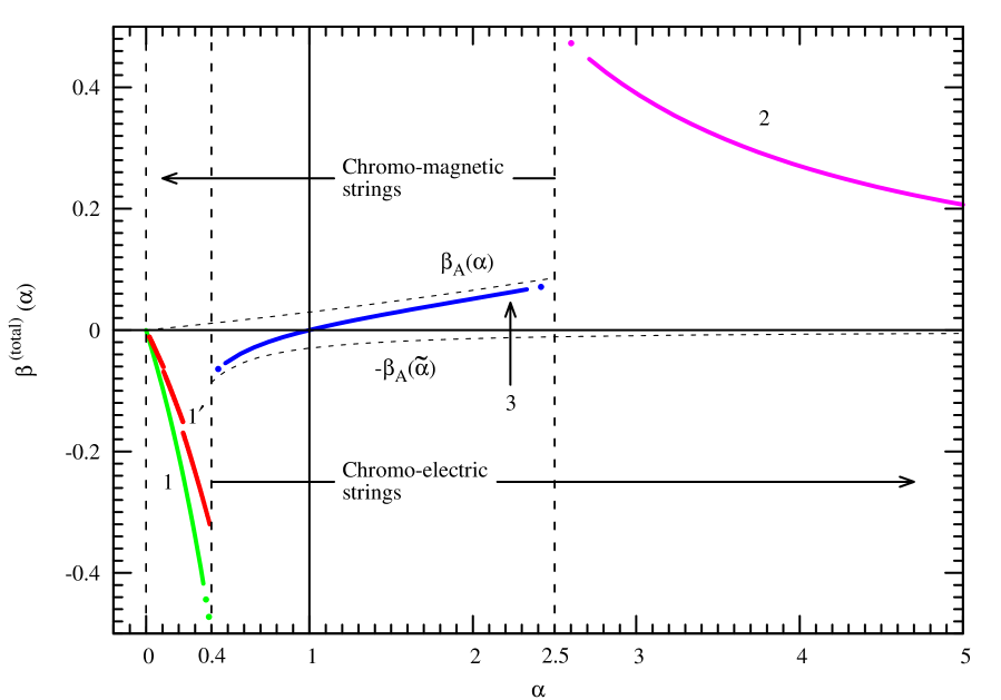
Fig. 7: The total $\beta$–function for QCD and pure $SU(3)\times\widetilde{SU(3)}$ color gauge theory (gluondynamics): (i) Curve 1 describes the perturbative $\beta$–function, corresponding to contributions of usual gluons, presented in (a) of Fig. 8. (ii) Curve 1’ corresponds to the perturbative QCD $\beta$–function (with quark and gluon contributions). (iii) Curve 2 describes the perturbative $\beta$–function, corresponding to contributions of dual gluons, presented by (b) of Fig. 8. (iv) Curve 3 describes a sum of contributions of scalar “monopoles”, given by $\beta_{A}(\alpha)$, and scalar monopoles, given by $-\beta_{A}(1/\alpha)$. Both of them exist in the non–perturbative region of gluondynamics, or QCD. The critical points: $\alpha_{1}\approx 0.4$ and $\alpha_{2}\approx 2.5$, and regions of the existence of chromo–electric (for $\alpha\geq 0.4$) and chromo–magnetic (for $\alpha\leq 2.5$) strings (ANO flux–tubes) are also shown in this figure. The total $\beta$–function has a zero at the point $\alpha=\tilde{\alpha}=1$, predicted by our model.

The behaviour of the total $\beta$–function for the pure $SU(3)\times\widetilde{SU(3)}$ colour gauge theory is given by Fig. 7, where the curve 1 describes the contribution of usual gluons for $\alpha<0.4$ (see (a) of Fig. 8), but a tail of $\beta^{total}(\alpha)$, corresponding to $\alpha>2.5$, is described by the curve 2, which presents loop contributions of diagrams in (b) of Fig. 8. The curve 1’ describes the perturbative QCD $\beta$–function with quark and gluon contributions. The curve 3 presents a sum of contributions of scalar “monopoles” given by function $\beta_{A}(\alpha)$, and scalar monopoles described by function $-\beta_{A}(1/\alpha)$. Both of them exist in the non–perturbative region of gluondynamics, or QCD. The critical points: $\alpha_{1}\approx 0.4$ and $\alpha_{2}\approx 2.5$ also are shown in Fig. 7. Of course, we do not know the behaviour of the total $\beta$–function near the phase transition points. But these points explain an approximate freezing of $\alpha$ in the region (81), where both charges, chromo–electric and chromo–magnetic ones, are confined. Chromo–electric strings exist for $\alpha>0.4$, and chromo–magnetic ones exist for $\alpha<2.5$. The region of strings is shown in Fig. 7. Also we see that the total $\beta$–function has a zero at the point $\alpha=\tilde{\alpha}=1$, predicted by our $SU(3)\times\widetilde{SU(3)}$ gauge theory. The behaviour of the total $\beta$–function, given by Fig. 7, is valid in the case of dyons, for which we have the same RGEs.

The ideas of Refs. [19, 20] are also valid in the case of the Family replicated gauge group models (see, for example, Refs. [80, 81] and the review [82, 83]), where magnetic charges of monopoles (or dyons) are essentially diminished in comparison with those of the SM. We have left these models for future investigations.

In the pure $SU(3)\times\widetilde{SU(3)}$ gauge theory there is no region of $\alpha$ when the perturbative expansions over $g$ and $\tilde{g}$ exist simultaneously: when the non–dual sector is unconfined, then the dual sector is entirely confined and vice versa. Such a situation takes place also in the case of non–abelian theories with matter fields.

9 Nonabelian theories with matter fields

Let us consider now nonabelian theories with matter fields having charge $ng$, or dual charge $n\tilde{g}$ (monopoles), or both of them (dyons).

If a surface $\Sigma$ in spacetime is parameterized as a closed loop in loop space, then via Eq. (14) it corresponds to a closed loop $\Gamma_{\Sigma}$ in the gauge group $G_{g}$. We say that the surface $\Sigma$ encloses a monopole if $\Gamma_{\Sigma}$ is in a non–trivial homotopy class of $G_{g}$. This generalizes the Dirac magnetic monopole [84] to the nonabelian case.

If matter fields, both non–dual and dual, exist in the nonabelian gauge theory, then a total system of fields is described by the action having the following structure:

$$S^{(total)}=S+S_{(m)}+S_{(d.m.)},$$ (86)

where $S$ is the Zwanziger–type action (22) for gauge fields, $S_{(m)}$ is an action of matter fields, and $S_{(d.m.)}$ describes dual matter fields (monopoles). For dyons we have:

$$S^{(total)}=S+S_{D},$$ (87)

where $S_{D}$ is an action of dyon matter fields. Then (apart of dyons):

$$S^{(total)}\approx S^{(n/d)}+S_{(m)}\qquad\mbox{for}\qquad\alpha<1,$$ (88)

and

$${\tilde{S}}^{(total)}\approx S^{(d)}+S_{(d.m.)}\qquad\mbox{for}\qquad\alpha>1,$$ (89)

where $S_{(n/d,d)}$ are non–dual and dual actions of gauge fields.

Nonabelian theories, revealing the (generalized) dual symmetry, have the following properties:

1. Monopoles of $A_{\mu}$ are charges of ${\tilde{A}}_{\mu}$, and “monopoles” of $\tilde{A}_{\mu}$ are charges of $A_{\mu}$.

2. If monopoles, as well as the charged particles, are Dirac fermions, then they are described by the Dirac Lagrangians:

   $$L_{(m)}={\bar{\psi}}\gamma_{\mu}(iD_{\mu}-m)\psi,$$ (90)

   $$L_{(d.m.)}={\bar{\chi}}\gamma_{\mu}(i{\tilde{D}}_{\mu}-\tilde{m})\chi,$$ (91)

   where covariant derivatives $D_{\mu}$ and ${\tilde{D}}_{\mu}$ are given by Eqs. (59).

   The action of matter fields is:

   $$S_{(m)\qquad\mbox{or}\qquad(d.m.)}=\int d^{4}xL_{(m)\qquad\mbox{or}\qquad(d.m.)}.$$ (92)

3. Charged particles and monopoles can be the Klein–Gordon complex scalars:

   $$L_{(m)}=\frac{1}{2}[{|D_{\mu}\phi|}^{2}-m^{2}{|\phi|}^{2}],$$ (93)

   $$L_{(d.m.)}=\frac{1}{2}[{|{\tilde{D}}_{\mu}\tilde{\phi}|}^{2}-{\tilde{m}}^{2}{|\tilde{\phi}|}^{2}],$$ (94)

   or Higgs scalars:

   $$L_{(m)}=\frac{1}{2}[{|D_{\mu}\phi|}^{2}-U(|\phi|)],$$ (95)

   $$L_{(d.m.)}=\frac{1}{2}[{|{\tilde{D}}_{\mu}\tilde{\phi}|}^{2}-U(|\tilde{\phi}|)],$$ (96)

   where

   $$U(|\phi|)=\frac{1}{2}m^{2}{|\phi|}^{2}+\frac{\lambda}{4}{|\phi|}^{4},$$ (97)

   and

   $$U(|\tilde{\phi}|)=\frac{1}{2}{\tilde{m}}^{2}{|\tilde{\phi}|}^{2}+\frac{\tilde{\lambda}}{4}{|\tilde{\phi}|}^{4}$$ (98)

   are the Higgs potentials.

   All these matter fields can belong to different (for example, fundamental or adjoint) representations of $SU(N)$ group. In Refs. [14, 15, 16, 17, 18, 19] monopoles belong to the fundamental representation of $SU(N)$.

   For dyons – particles having both, electric and magnetic, charges simultaneously – we have in Eqs. (90-98):

   $$\psi^{ap}\equiv\chi^{ap}$$ (99)

   and

   $$\phi^{ap}\equiv\tilde{\phi}^{ap},$$ (100)

   where $a,p$ are non–dual and dual indices of the $SU(N)$ and $\widetilde{SU(N)}$ representations respectively.

4. The charges of matter fields $g_{m}$ and ${\tilde{g}}_{m}$ satisfy the charge quantization condition:

   $$g_{m}{\tilde{g}}_{m}=4\pi n,\qquad n\in Z,$$ (101)

   if matter fields belong to the adjoint representation of $SU(N)$ group. The Dirac relation:

   $$g_{m}{\tilde{g}}_{m}=2\pi n,\qquad n\in Z,$$ (102)

   takes place for matter fields transforming according to fundamental representations (see Ref. [12, 13]). In general, we always have the following condition:

   $$\alpha(\mu)\tilde{\alpha}(\mu)={\mbox{const}},$$ (103)

   which is valid at arbitrary energies $\mu$.

We have no dual fundamental matter fields in the SM. No experimental indications for any (abelian or non–abelian) fundamental monopoles or dyons. May be they exist at high energy scales.

Considering QCD, we have quarks belonging to the triplet representation of $SU(3)$ colour gauge group, but light monopoles, belonging to the triplet representation of $\widetilde{SU(3)}$, are experimentally absent. By this reason, we have no dual symmetry for the total QCD. There exists only a dual symmetry of its gauge field part. The total QCD $\beta$–function is presented by curves 1’, 2 and 3 of Fig. 7, instead of curves 1, 2, 3 describing by gluondynamics.

10 Running $\alpha_{s}^{-1}(\mu)$

Considering Eq. (45) for QCD regions 1’, 2 and 3 of Fig. 7, we obtain the following results.

1. For the region 1’ we have:

   $$\frac{\mbox{d}\ln\alpha(t)}{\mbox{dt}}=\beta(\alpha),$$ (104)

   where $\beta(\alpha)$ ($\alpha\equiv\alpha_{s}$) is given by Eqs. (50) and (52) with $N_{f}=3,4,5$ up to the point $\mu=M_{Z}$. The solution of Eq. (104) in the 3–loop approximation has the following expression (see for example [85, 86]):

   $$\alpha^{-1}(\mu)=\alpha^{-1}(\mu_{R})+\frac{\beta_{0}}{4\pi}t+\lambda_{1}\ln\frac{\alpha^{-1}(\mu)+\lambda_{1}}{\alpha^{-1}(\mu_{R})+\lambda_{1}}\qquad{\mbox{for}}\qquad\alpha<0.4,$$ (105)

   where $\mu_{R}$ is the renormalization point and:

   $$\lambda_{1}=\frac{1}{4\pi}\frac{\beta_{1}}{\beta_{0}}.$$ (106)

2. For the region 2 we have:

   $$\frac{\mbox{d}\ln\alpha(t)}{\mbox{dt}}=-\beta(\tilde{\alpha})=-\beta(1/\alpha)$$ (107)

   where $\beta(\tilde{\alpha})$ is given by Eqs. (50) and (51). The solution of this equation gives the following behaviour:

   $$\alpha^{-1}(\mu)=\left[\alpha^{-1}(\mu_{R})+\frac{\beta_{0}}{4\pi}t+\lambda_{1}\ln\frac{\alpha^{-1}(\mu)+\lambda_{1}}{\alpha^{-1}(\mu_{R})+\lambda_{1}}\right]^{-1}\qquad{\mbox{for}}\qquad\alpha>2.5,$$ (108)

   where $\beta_{0}$ and $\lambda_{1}$ correspond to $N_{f}=0$.

3. For the region 3 of Fig. 7 we have Eq. (83), calculated according to the MAP–method. Curve 3 describes a sum of contributions of scalar monopoles given by $\beta_{A}(\alpha)$, and scalar “monopoles” given by $-\beta_{A}(1/\alpha)$.

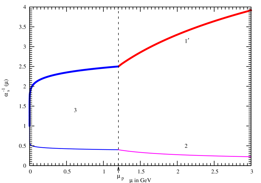
Fig. 9: The evolution of the inversed $\alpha(\mu)\equiv\alpha_{s}(\mu)$. A solid curve corresponds to the curve 1’ and first part of region 3 of Fig. 7. A thin curve corresponds to the region 2 and second part of the same region 3 of Fig. 7. The solutions, presented by this curve, are not realized in QCD: they describe the evolution of the inversed $\tilde{\alpha}$. In the non–perturbative region, the solid curve 3 approaches to the point $\alpha(0)=1$. We see the sharp decreasing of $\alpha^{-1}(\mu)$ near this point.

The results of all these solutions (also valid for dyons) are presented by Fig. 9 for the evolution of $\alpha_{s}^{-1}(\mu)$. The value $\mu_{p}\approx 1.2$ GeV, shown in Fig. 9, corresponds to the end of perturbation region 1’ (or 1) and the beginning of confinement region 3. In the non–perturbation region 3, we have a solution given by solid curve 3 of Fig. 9, which approaches the point $\alpha_{s}(\mu)=1$ when $\mu\to 0$, and we see a rapid decrease of $\alpha^{-1}(\mu)$ near 1.

It seems that solutions presented in Fig. 9 by thin curves, which correspond to the region 2 and second part of the region 3 of Fig. 7, are not realized in QCD: they describe the running of inverse $\tilde{\alpha}$. We see that the dual part of QCD does not play an essential role in the formation of QCD vacuum: mainly monopoles, or magnetic part of dyons, participate in the formation of electric “strings” – ANO flux tubes, although solid curves 3 of Fig. 7 and Fig. 9 present the contributions of both parts, electric and magnetic ones.

As it was shown in Refs. [87, 88, 89] (and developed in Refs. [85, 86]), the QCD effective Lagrangian is given by the following expression:

$$L_{eff}=-\frac{\alpha_{eff}^{-1}(F^{2})}{16\pi}F^{2},\qquad{\mbox{where}}\qquad F^{2}=F_{\mu\nu}^{J}F_{\mu\nu}^{J}\qquad(J=1,2,..8).$$ (109)

This Lagrangian contains the effective fine structure constant:

$$\alpha_{eff}(F^{2})=\frac{g^{2}_{eff}}{4\pi},$$ (110)

which in general is a complicated nonlinear function of gluon fields. In the perturbative region $\alpha_{eff}(F^{2})$ coincides with the running of $\alpha_{eff}(\mu)$, where $F^{2}=(\mu$ GeV)⁴ (see Refs. [85, 86, 87, 88, 89]). But in the non–perturbative region we have a nontrivial situation: for asymptotically free theories the maximum of the effective action (e.g. minimum of the effective potential) already does not correspond to the classical vacuum with $F^{2}=0$. The quantum fluctuations lead to the formation of a gluon condensate (QCD vacuum). In our approach the gluon condensate $F_{0}^{2}=(\mu^{*}_{cond}$ GeV)⁴ corresponds to the maximal value of $\alpha_{s}$ equal to 1. By this reason, we suppose that the variable $F^{2}$ is not given by $\mu^{4}$ in the non-perturbation region. Instead of $\mu$, it is natural to consider the following variable:

$$\mu^{*}=\mu+\mu^{*}_{cond}\sim\frac{1}{r},$$ (111)

which determines distances r, and we have:

$$F^{2}=(\mu^{*}\,\,{\mbox{GeV}})^{4}.$$ (112)

The nature of gluon condensate was investigated in a lot of papers (for example, very interesting considerations were given in Refs. [90, 91]).

The value of gluon condensate was estimated in Refs. [92, 93, 94]:

$$\left\langle\frac{\alpha_{s}}{4\pi}F^{2}_{0}\right\rangle\approx 0.012\,\,{\mbox{GeV}^{4}}.$$ (113)

For our case $\alpha_{s}=1$, and we have:

$$F^{2}_{0}\approx 0.15\,\,{\mbox{GeV}^{4}},$$ (114)

or

$$\mu^{*}_{cond}\approx 0.62\,\,{\mbox{GeV}}.$$ (115)

The behaviour of inversed $\alpha(\mu)$ presented in Fig. 9 shows that in the region 3 given by solid curve we have:

$$\alpha\simeq 0.45\pm 0.05,$$ (116)

e.g. almost unchanged (“freezing”) $\alpha$ for a wide interval of $\mu^{*}$:

$$0.72\,\,{\mbox{GeV}}\lesssim\mu^{*}\lesssim 1.82\,\,{\mbox{GeV}}.$$ (117)

We see that QCD, including its dual sector, acquires a new comprehension.

11 The effective potential in QCD

The perturbative effective potential is given by the following expression (see Refs. [85, 86, 87, 88, 89]):

$$V_{eff}=\frac{\alpha_{eff}^{-1}(F^{2})}{16\pi}F^{2}\qquad{\mbox{with}}\qquad F^{2}=(\mu\,\,{\mbox{GeV}})^{4}.$$ (118)

However, this expression is not valid in the non–perturbative region, because the non–perturbative vacuum contains a condensation of chromo–magnetic flux tubes, according to so called “spaghetti vacuum” by Nielsen–Olesen [95]. By this reason, we subtract the contribution of “strings”, determined by the gluon condensate $F_{0}^{2}$, from the expression (118):

$$V_{eff}=\frac{\alpha_{eff}^{-1}(F^{2})}{16\pi}F^{2}-\frac{\alpha_{eff}^{-1}(F_{0}^{2})}{16\pi}F_{0}^{2},$$ (119)

using $F^{2}=(\mu^{*}$ GeV)⁴.

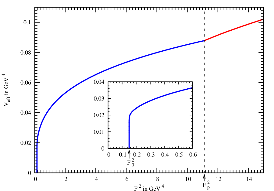
Fig. 10: The effective potential of $SU(3)\times\widetilde{SU(3)}$ color gauge theory, as a function of $F^{2}$. The point $F^{2}=F_{0}^{2}\approx 0.15$ GeV⁴ corresponds to the gluon condensate. Near this point the effective potential has a sharp minimum, corresponding to the first order phase transition in the deep non–perturbative region, far from its beginning $F_{p}^{2}$.

The behaviour of the effective potential $V_{eff}(F^{2})$ is given by Fig. 10, and we see: The QCD effective potential shows a sharp minimum in the deep non–perturbative region (at the point $F^{2}=F^{2}_{0}=0.15$ GeV⁴). This minimum points out the existence of the (unexpected) first order phase transition in QCD at the point $\mu^{*}_{cond}\approx 0.62$ GeV.

12 Conclusions

In the present paper we have obtained the following results:

1. The Zwanziger–type action can be constructed for nonabelian theories revealing the generalized dual symmetry. In the abelian limit this action corresponds to the Zwanziger formalism for quantum electro–magneto dynamics (QEMD). It was emphasized that although the generalized dual transformation is rather complicated, it is explicit in terms of loop space variables.

2. We have shown that the Zwanziger–type action confirms the invariance under the interchange:

   $$\alpha\leftrightarrow\tilde{\alpha}=\frac{1}{\alpha}.$$

3. Such a symmetry leads to the generalized renormalization group equations:

   $$\frac{\mbox{d}\ln\alpha(t)}{\mbox{dt}}=-\frac{\mbox{d}\ln{\tilde{\alpha}}(t)}{\mbox{dt}}=\beta(\alpha)-\beta(\tilde{\alpha})=\beta^{(total)}(\alpha),$$

   where $\beta^{(total)}(\alpha)$ is the total $\beta$–function, antisymmetric under the interchange:

   $$\alpha\leftrightarrow\tilde{\alpha},\qquad{\mbox{or}}\qquad\alpha\leftrightarrow\frac{1}{\alpha}$$

   for pure nonabelian theories.

4. We have applied the method of Maximal Abelian Projection (MAP) by t’ Hooft to the pure $SU(3)$ gauge theory with aim to describe the behaviour of the total $\beta$–function in the region $0\leq\alpha,\tilde{\alpha}<\infty$.

5. We have shown that as a result of the dual symmetry and MAP $\beta^{(total)}(\alpha)$ has a zero at $\alpha=\tilde{\alpha}=1$ (“fixed point”):

   $$\beta^{(total)}(\alpha=\tilde{\alpha}=1)=0.$$

6. At the first step, we have considered the existence of the $N-1$ Higgs abelian scalar monopole fields ${\tilde{\phi}}_{1,2,...,N-1}$ and $N-1$ Higgs abelian scalar electric fields $\phi_{1,2,...,N-1}$ in the non–perturbative region of pure nonabelian $SU(N)\times\widetilde{SU(N)}$ gauge theories.

7. At the second step, we have assumed that a generalized dual symmetry naturally leads to the existence of the Higgs scalar dyon fields $\phi_{1,2,...,N-1}$, which are created by non–perturbative effects of the $SU(N)\times\widetilde{SU(N)}$ gluondynamics. These abelian dyons have both (electric and magnetic) charges, and describe the total $\beta$–function in the following non–perturbative region:

   $$0.4<\alpha<2.5,$$

   which explains the freezing of $\alpha_{s}$ in QCD.

8. We also discussed the case of nonabelian theories with matter fields, which in general have no dual symmetry.

9. We have investigated the running of $\alpha_{s}^{-1}(\mu)$ in the perturbative and non–perturbative regions of $\mu$.

10. We have calculated the value of the gluon condensate: $F_{0}^{2}\approx 0.15$ GeV⁴, in accord with the well–known result, given by literature.

11. We have presented the behaviour of the QCD effective potential as a function of $F^{2}$, having a sharp minimum in the non–perturbative region. This minimum, corresponding to the gluon condensate, prompts the existence of the first order phase transition in QCD.

Appendix A: The regularization procedure

With aim to understand the difference between the quantities $F_{\mu}[\xi|s]$ and $E_{\mu}[\xi|s]$, it is convenient to give some explanations, coming from Refs. [14, 15, 16, 17, 18, 19]. The new variables $E_{\mu}[\xi|s]$ are not gauge invariant like $F_{\mu}[\xi|s]$. But in spite of this inconvenient property, the variables $E_{\mu}[\xi|s]$ are more useful for studying the generalized duality. They can be represented as the bold curve in Fig. 4 where the phase factors $\Phi_{\xi}(s,0)$ cancel parts of the faint curve representing $F_{\mu}[\xi|s]$. The loop derivative considered in this paper is defined as

$$\frac{\delta\Phi[\xi]}{\delta\xi^{\mu}(s)}=\lim_{\Delta\to 0}\frac{\Phi[\xi^{\prime}]-\Phi[\xi]}{\Delta},$$ (A.1)

where

$${\xi^{\prime}}^{\lambda}={\xi}^{\lambda}(s^{\prime})+\Delta\delta^{\lambda}_{\mu}\delta(s-s^{\prime}).$$ (A.2)

The $\delta$–function $\delta(s-s^{\prime})$ is a bump function centred at s with width $\epsilon=s_{+}-s_{-}$ (see Fig. 4). In contrast to $F_{\mu}[\xi|s]$, the quantity $E_{\mu}[\xi|s]$ depends only on a “segment” of the loop $\xi^{\mu}(s)$ from $s_{-}$ to $s_{+}$. The regularization of $\delta$–function is necessary for the definition of loop derivatives used in this theory. The quantities $E_{\mu}[\xi|s]$, constrained by the condition:

$$\frac{\delta E_{\mu}[\xi|s]}{\delta\xi^{\nu}}-\frac{\delta E_{\nu}[\xi|s]}{\delta\xi^{\mu}}=0,$$ (A.3)

constitute a set of the curl–free variables valid for the description of nonabelian theories revealing properties of the generalized dual symmetry.

Appendix B: Renormalization group equation for non-dual and dual coupling constants

The renormalization group (RG) describes an independence of a theory and its couplings on an arbitrary scale parameter $M$. We are interested in RG applied to the effective potential depending on scalar field $\phi$. The renormalization group equation (RGE) for the effective potential means that the potential cannot depend on a change in the arbitrary renormalization scale parameter $M$:

$$\frac{dV_{eff}}{dM}.$$ (B.1)

The effects of changing it are absorbed into changes in the coupling constants, masses and fields, giving so–called running quantities. Knowing the dependence on $M^{2}$ is equivalent to knowing the dependence on $\phi^{2}$. This dependence is given by RGE. Considering the RGE improvement of the potential, we follow the approach by Coleman and Weinberg [97] (see also the review [98]) for scalar electrodynamics and its extension to the massive theory [99]. Here we have the difference between the scalar electrodynamics [97] and scalar QuantumElectroMagnetoDynamics (QEMD) when we have scalar particles with electric charge $e$ and scalars with magnetic charge $g$.

RGE for the improved one–loop effective potential can be given in QEMD by the following expression:

$$\left(M\frac{\partial}{\partial M}+\beta_{\lambda}\frac{\partial}{\partial\lambda}+e\beta_{e}\frac{\partial}{\partial e}+g\beta_{g}\frac{\partial}{\partial g}+\beta_{(m^{2})}{m^{2}}\frac{\partial}{\partial m^{2}}-\gamma\phi\frac{\partial}{\partial\phi}\right)V_{eff}(\phi^{2})=0,$$ (B.2)

where the function $\gamma$ is the anomalous dimension:

$$\gamma\left(\frac{\phi}{M}\right)=-\frac{\partial\phi}{\partial M}.$$ (B.3)

RGE (B.2) leads to a new improved effective potential [97]:

$$V_{eff}(\phi^{2})=\frac{1}{2}m^{2}_{ren}(t)G^{2}(t)\phi^{2}+\frac{1}{4}\lambda_{ren}(t)G^{4}(t)\phi^{4},$$ (B.4)

where

$$G(t)\equiv\exp\left[-\frac{1}{2}\int_{0}^{t}dt^{\prime}\gamma(g_{ren}(t^{\prime}),\lambda_{ren}(t^{\prime}))\right].$$ (B.5)

Eq. (B.2) reproduces also a set of ordinary differential equations:

$$\frac{d\lambda_{ren}}{dt}=\beta_{\lambda}(g_{ren}(t),\lambda_{ren}(t)),$$ (B.6)

$$\frac{dm^{2}_{ren}}{dt}=m^{2}_{ren}(t)\beta_{(m^{2})}(g_{ren}(t),\lambda_{ren}(t)),$$ (B.7)

$$\frac{d\ln e_{ren}}{dt}=-\frac{d\ln g_{ren}}{dt}=\beta_{e}(g_{ren}(t),\lambda_{ren}(t))-\beta_{g}(g_{ren}(t),\lambda_{ren}(t))\equiv\beta^{(total)},$$ (B.8)

where $t=\ln(\phi^{2}/{M^{2}})$, and the subscript “ren” means the “renormalized” quantity.

The last equation (B.8) is obtained with the help of the Dirac relation $eg=2\pi n$ $(n\in Z)$ for minimal charges when $eg=2\pi$. Indeed, in Eq. (B.2):

$$e\beta_{e}\frac{\partial}{\partial e}+g\beta_{g}\frac{\partial}{\partial g}=e\beta_{e}\frac{\partial}{\partial e}+g\beta_{g}\frac{de}{dg}\frac{\partial}{\partial e}=\left(e\beta_{e}+g\beta_{g}\left(-\frac{2\pi}{g^{2}}\right)\right)\frac{\partial}{\partial e}$$

$$=(\beta_{e}-\beta_{g})\frac{\partial}{\partial\ln e}=\beta^{(total)}\frac{\partial}{\partial\ln e},$$ (B.9)

where

$$\beta^{(total)}=\beta_{e}-\beta_{g}.$$ (B.10)

Using fine structure constants

$$\alpha=\frac{e^{2}}{4\pi},\qquad\tilde{\alpha}=\frac{g^{2}}{4\pi},$$ (B.11)

we obtain Eq.(45) given in Section 5. But for abelian theories we have $\alpha\tilde{\alpha}=1/4$.

Eq.(45) takes place also for nonabelian theories with charge quantization condition $g\tilde{g}=4\pi n$ $(n\in Z)$ giving $\alpha\tilde{\alpha}=1$.

Appendix C: Abelian projection method

In this Appendix we present the method of the Maximal Abelian Projection (MAP) by G. t’ Hooft [43], following the review [45].

For any composite field $X$ (for example, $F_{\mu\nu}$) transforming as an adjoint representation

$$X\to X^{\prime}=VXV^{-1},$$ (C.1)

we can find the specific unitary matrix $V$ (the gauge), where $X$ is diagonal:

$$X^{\prime}=VXV^{-1}=diag(\lambda_{1},\lambda_{2},...\lambda_{N}).$$ (C.2)

For $X$ from the Lie algebra of $SU(N)$, one can choose $\lambda_{1}\leq\lambda_{2}\leq\lambda_{3}\leq...\lambda_{N}$. It is clear that $V$ is determined up to the left multiplication by a diagonal $SU(N)$, which belongs to the Cartan (or largest abelian) subgroup of $SU(N)$:

$$U(1)^{N-1}\subset SU(N).$$ (C.3)

Now we transform $A_{\mu}$, according to the gauge (C.2):

$$\tilde{A}_{\mu}=V\left(A_{\mu}+\frac{i}{g}\partial_{\mu}\right)V^{-1}$$ (C.4)

and consider the transformations of $\tilde{A}_{\mu}$ under $U(1)^{N-1}$. The diagonal components

$$a^{i}_{\mu}\equiv(\tilde{A}_{\mu})_{i}^{i}\qquad(i=1,2,3)$$ (C.5)

transform as “photons”:

$$a_{\mu}^{i}\to a^{i}_{\mu}=a^{i}_{\mu}+\frac{1}{g}\partial_{\mu}\alpha_{i},$$ (C.6)

while nondiagonal, $c_{\mu}^{ij}\equiv A_{\mu}^{ij}$, transform as charged fields:

$$C^{{}^{\prime}ij}_{\mu}=\exp[i(\alpha_{i}-\alpha_{j})]C_{\mu}^{ij}.$$ (C.7)

By ’t Hooft remarks [43], this is not the whole story: there appear singularities due to a possible coincidence of two or more eigenvalues $\lambda_{i}$, which leads to the existence of monopoles. To make it explicit, let us consider (as in [43]) the “photon” field strength:

$$f^{i}_{\mu\nu}=\partial_{\mu}a^{i}_{\nu}-\partial_{\nu}a^{i}_{\mu}$$

$$=VF_{\mu\nu}V^{-1}+ig\left[V\left(A_{\mu}+\frac{i}{g}\partial_{\mu}\right)V^{-1},V\left(A_{\nu}+\frac{i}{g}\partial_{\nu}\right)V^{-1}\right],$$ (C.8)

and define the monopole current:

$$K^{i}_{\mu}=\frac{1}{8\pi}\varepsilon_{\mu\nu\rho\sigma}\partial_{\nu}f^{i}_{\rho\sigma},\qquad\partial_{\mu}K^{i}_{\mu}=0.$$ (C.9)

Since $F_{\mu\nu}$ is regular, the only singularity giving rise to $K^{i}_{\mu}$ is the commutator term in (C.8), otherwise the smooth part of $a^{i}_{\mu}$ does not contribute to $K^{i}_{\mu}$ because of the antisymmetric tensor.

Hence one can define the magnetic charge $m^{i}(\Omega)$ in the $3d$ region $\Omega$:

$$m^{i}(\Omega)=\int_{\Omega}d^{3}\sigma_{\mu}K^{i}_{\mu}=\frac{1}{8\pi}\int_{\partial\Omega}d^{2}\sigma_{\mu\nu}\varepsilon_{\mu\nu\rho\sigma}f^{i}_{\rho\sigma}.$$ (C.10)

Let us consider now the situation when two eigenvalues of (C.2) coincide, e.g. $\lambda_{1}=\lambda_{2}$. This may happen at one $3d$ point in $\Omega$, $x^{(1)}$, i.e. on the line in the $4d$, which one can visualize as the magnetic monopole world line. The contribution to $m^{i}(\Omega)$ comes only from the infinitesimal neighbourhood $B_{\varepsilon}$ of $x^{(1)}$:

$$m^{i}(B_{\varepsilon}(x^{(1)})) = \frac{i}{4\pi}\int_{S_{\varepsilon}}d^{2}\sigma_{\mu\nu}\varepsilon_{\mu\nu\rho\sigma}\left[V\partial_{\rho}V^{-1},V\partial_{\sigma}V^{-1}\right]_{ii}$$ (C.11)

$$= -\frac{i}{4\pi}\int d^{2}\sigma_{\mu\nu}\varepsilon_{\mu\nu\rho\sigma}\partial_{\rho}\left[V\partial_{\sigma}V^{{}_{1}}\right]_{ii}.$$

The term $V\partial_{\sigma}V^{-1}$ is singular and should be treated with care. To make it explicit, one can write:

$$V=W\left(\begin{array}[]{cc}\cos\frac{1}{2}\theta+i\vec{\sigma}\vec{e}_{\phi}\sin\frac{\theta}{2}&0\\ 0&1\end{array}\right),$$ (C.12)

where $W$ is a smooth $SU(N)$ function near $x^{(1)}$. Inserting it in (C.11), one obtains:

$$m^{i}(B_{\varepsilon}(x^{(1)}))=\frac{1}{8\pi}\int_{S_{\varepsilon}}d^{2}\sigma_{\mu\nu}\varepsilon_{\mu\nu\rho\sigma}\partial_{\rho}(1-\cos\theta)\partial_{\sigma}\phi[\sigma_{3}]_{ii},$$ (C.13)

where $\phi$ and $\theta$ are azimuthal and polar angles. The integrand in (C.13) is a Jacobian displaying a mapping from $S^{2}_{\varepsilon}(x^{(1)})$ to $(\theta,\phi)\sim SU(2)/U(1)$. Since

$$\Pi_{2}\left(\frac{SU(2)}{U(1)}\right)=Z,$$ (C.14)

the magnetic charge is $m^{i}=0,\pm 1/2,\pm 1,..$.

From the derivation above it is clear, that the point $x=x^{(1)}$, where $\lambda_{1}(x^{(1)})=\lambda_{2}(x^{(1)}),$ is a singular point of the gauge transformed $A_{\mu}$ and $a^{i}_{\mu}$, and the latter behaves near $x=x^{(1)}$ as $0(1/|x-x^{(1)}|)$, and abelian projected field strength $f^{i}_{\mu\nu}$ is $0(1/|x-x^{(1)}|^{2})$, similar to the magnetic field of a point–like magnetic monopole. However, several properties should be stressed now:

1. The original vector potential $A_{\mu}$ and $F_{\mu\nu}$ are smooth and do not show any singular behaviour.

2. At large distances $f^{i}_{\mu\nu}$ is not, generally speaking, monopole–like, i.e. does not decrease as $1/|x-x^{(1)}|^{2}$, so that similarity to the magnetic monopole (its topological properties) can be seen only in the vicinity of the singular point $x^{(1)}$.

3. In general, monopoles considered by MAP–method have nothing to do with classical solutions: MAP–monopoles are quantum fluctuations of gluon fields. Actually almost any field distribution in the vacuum may be abelian projected into $a_{\mu}^{i},f_{\mu\nu}^{i}$ and then magnetic monopoles can be detected.

Fig. 1: The closed loop $C$ with coordinates $\xi^{\mu}(s)$ and loop parameter s: $0\leq s\leq 2\pi$.

Fig. 2: The closed loop $\tilde{C}$ with coordinates $\eta^{\mu}(t)$ and loop parameter t: $0\leq t\leq 2\pi$.

Fig. 3: The illustration of the quantity $F_{\mu}[\xi|s]$.

Fig. 4: The illustration of the quantity $E_{\mu}[\xi|s]$.

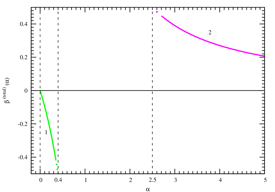
Fig. 5: The perturbative $\beta$–functions of the pure $SU(3)\times\widetilde{SU(3)}$ color gauge theory: $\beta(\alpha)$ – curve 1, and $-\beta(\tilde{\alpha})=-\beta(1/\alpha)$ – curve 2.

Fig. 6: The one–loop corrections: (a) from electric “monopoles” to the gluon propagator, and (b) from monopoles to the dual gluon propagator.

Fig. 8: The loop contributions to the gluon propagator (without matter fields): (a) the contributions from usual gluons, and (b) the contributions from dual gluons.

References

- [1] S. Mandelstam, Phys.Rev. D11, 3026 (1975).
- [2] G. ’t Hooft, Nucl.Phys. B138, 1 (1978).
- [3] J. Maldacena, Adv.Theor.Math.Phys. 2, 231 (1998); arXiv: hep-th/9711200.
- [4] M.B. Halpern, Phys.Rev. D16, 1798 (1977).
- [5] M.B. Halpern, Phys.Rev. D16, 3515 (1977).
- [6] M.B. Halpern, Phys.Rev. D19, 517 (1979).
- [7] M.B. Halpern, Nucl.Phys. B139, 477 (1978).
- [8] G.G. Batrouni, Nucl.Phys. B208, 12 (1982).
- [9] G.G. Batrouni, Nucl.Phys. B208, 467 (1982).
- [10] G.G. Batrouni and M.B. Halpern, Phys.Rev. D30, 1782 (1984).
- [11] H.M. Chan and S.T. Tsou, An Electric–Magnetic Duality for Non–Abelian Yang–Mills Fields, The 28th Int.Conf. on High–energy Physics, Warsaw 1996, ICHEP’96, Vol.2, p.1654.
- [12] P. Di Vecchia, Surveys in High Energ.Phys. 10, 119 (1997); hep-th/9608090.
- [13] P. Di Vecchia, Duality in N=2,4 Supersymmetric Gauge Theories, arXiv: hep-th/9803026.
- [14] H.M. Chan, J. Faridani and S.T. Tsou, Phys.Rev. D52, 6134 (1995); arXiv: hep-th/9503106.
- [15] H.M. Chan and S.T. Tsou, Phys.Rev. D56, 3646 (1997); arXiv: hep-th/9702117.
- [16] H.M. Chan and S.T. Tsou, Phys.Rev. D57, 2507 (1998); arXiv: hep-th/9701120.
- [17] H.M. Chan, J. Faridani and S.T. Tsou, Phys.Rev. D51, 7040 (1995).
- [18] H.M. Chan, J. Faridani and S.T. Tsou, Phys.Rev. D53, 7293 (1996); arXiv: hep-th/9512173.
- [19] S.T. Tsou, Int.J.Mod.Phys. A18S2, 1 (2003); arXiv: hep-th/0110256.
- [20] J. Bordes, H.M. Chan and S.T. Tsou, Updates of the dualized Standard Model in fermion masses and mixings, arXiv: hep-ph/0302199.
- [21] F. Fucito, M. Martellini and M. Zeni, Nucl.Phys. B496, 259 (1997); arXiv: hep-th/9605018.
- [22] A. Noguchi and A. Sugamoto, VESTNIK of the Tomsk State Pedagogical University, Special isuue, 44N7, 59 (2004); arXiv: hep-th/0408045.
- [23] A.M. Polyakov, Nucl.Phys. B164, 171 (1980).
- [24] D. Zwanziger, Phys.Rev. 176, 1489 (1968).
- [25] D. Zwanziger, Phys.Rev. D3, 880 (1971).
- [26] R.A. Brandt, F. Neri and D. Zwanziger, Phys.Rev. D19, 1153 (1979).
- [27] F.V. Gubarev, M.I. Polikarpov and V.I. Zakharov, Phys.Lett. B438, 147 (1998); arXiv: hep-th/9805175.
- [28] L.V. Laperashvili and H.B. Nielsen, Mod.Phys.Lett. A14, 2797 (1999); arXiv: hep-th/9910101.
- [29] G. t’ Hooft, Acta Physica Austrica suppl. XXII, 531 (1980).
- [30] C. Montonen and D. Olive, Phys.Lett. B72, 117 (1977).
- [31] M. Gell–Mann and F.E. Low, Phys.Rev. 95, 1300 (1954).
- [32] C.R. Das and L.V. Laperashvili, Phase transition in the Higgs model of scalar dyons, to be published in Mod.Phys.Lett. A, (2006); arXiv: hep-ph/0511067.
- [33] O.V. Tarasov, A.A. Vladimirov and A.Yu. Zharkov, Phys.Lett. B93, 429 (1980).
- [34] Yu.A. Simonov, Phys.Atom.Nucl. 58 107 (1995) [Yad.Fiz. 58, 113 (1995)]; arXiv: hep-ph/9311247.
- [35] A.M. Badalian and Yu.A. Simonov, Phys.Atom.Nucl. 60, 630 (1997) [Yad.Fiz. 60, 714 (1997)].
- [36] A.M. Badalian and D.S. Kuzmenko, Phys.Rev. D65, 016004 (2002); arXiv: hep-ph/0104097.
- [37] I.M. Narodetskii and M.A. Trusov, Phys.Atom.Nucl. 65, 917 (2002) [Yad.Fiz. 65, 949 (2002)]; arXiv: hep-ph/0104019.
- [38] I.M. Narodetskii and M.A. Trusov, Phys.Atom.Nucl. 67, 762 (2004) [Yad.Fiz. 67, 783 (2004)]; arXiv: hep-ph/0307131.
- [39] A.A. Abrikosov, Sov.Phys.JETP. 5, 1174, (1957) [Zh.Eksp.Teor.Fiz. 32, 1442 (1957)].
- [40] H.B. Nielsen and P. Olesen, Nucl.Phys. B61, 45 (1973).
- [41] L.V. Laperashvili, D.A. Ryzhikh and H.B. Nielsen, Int.J.Mod.Phys. A18, 4403 (2003); arXiv: hep-th/0211224.
- [42] C.R. Das and L.V. Laperashvili, Int.J.Mod.Phys. A20, 5911 (2005); arXiv: hep-ph/0503138.
- [43] G. ’t Hooft, Nucl. Phys. B190, 455 (1981).
- [44] A.S. Kronfeld, G. Schierholz and U.J. Wiese, Nucl.Phys. B293, 461 (1987).
- [45] Yu.A. Simonov, Phys.Usp. 39, 313 (1996) [Usp.Fiz.Nauk. 166, 337 (1996)]; arXiv: hep-ph/9709344.
- [46] L.D. Faddeev and A.J. Niemi, Phys.Lett. B525, 195 (2002); arXiv: hep-th/0101078.
- [47] M.N. Chernodub and F.V. Gubarev, JETP Lett. 62, 100 (1995); arXiv: hep-th/9506026.
- [48] G.S. Bali, C. Schlighter and K. Shilling, Prog.Theor.Phys.Suppl. 131, 645 (1998); arXiv: hep-lat/9802005.
- [49] M.N. Chernodub, F.V. Gubarev and M.I. Polikarpov, JETP Lett. 69, 169 (1999); arXiv: hep-lat/9801010.
- [50] M.N. Chernodub, Phys.Rev. D69, 094504 (2004); arXiv: hep-lat/0308031.
- [51] T. Suzuki, Prog.Theor.Phys. 80, 929 (1988).
- [52] S. Maedan and T. Suzuki, Prog.Theor.Phys. 81, 229 (1989).
- [53] M.N. Chernodub and M.I. Polikarpov, Abelian projections and monopoles in: “NATO Advanced Study Institute on Confinement, Duality and Non–perturbative Aspects of QCD”, Cambridge, England, 23 Jun - 4 Jul 1997, p.387: Ed. by Pierre van Baal, Plenum Press, 1998; arXiv: hep-th/9710205.
- [54] M.N. Chernodub, F.V. Gubarev, M.I. Polikarpov and A.I. Veselov, Prog.Theor.Phys.Suppl. 131, 309 (1998); arXiv: hep-lat/9802036.
- [55] M.N. Chernodub, F.V. Gubarev, M.I. Polikarpov and V.I. Zakharov, Phys.Atom.Nucl. 64, 561 (2001) [Yad.Fiz. 64, 615 (2001)]; arXiv: hep-th/0007135.
- [56] M.N. Chernodub, F.V. Gubarev, M.I. Polikarpov and V.I. Zakharov, Nucl.Phys. B600, 163 (2001); arXiv: hep-th/0010265.
- [57] M.N. Chernodub, F.V. Gubarev, M.I. Polikarpov and V.I. Zakharov, Nucl.Phys. B592, 107 (2001); arXiv: hep-th/0003138.
- [58] L.V. Laperashvili and H.B. Nielsen, Multiple Point Principle and phase transition in gauge theories, in: Proceedings of the International Workshop on “What Comes Beyond the Standard Model”, Bled, Slovenia, 29 June - 9 July, 1998 (DMFA, Zaloznistvo, Ljubljana, 1999), p.15; arXiv: hep-ph/9905357.
- [59] L.V. Laperashvili and H.B. Nielsen, Phase transition couplings in the Higgsed monopole model, arXiv: hep-th/9909181.
- [60] L.V. Laperashvili and H.B. Nielsen, Int.J.Mod.Phys. A16, 2365 (2001); arXiv: hep-th/0010260.
- [61] L.V. Laperashvili, H.B. Nielsen and D.A. Ryzhikh, Int.J.Mod.Phys. A16, 3989 (2001); arXiv: hep-th/0105275.
- [62] L.V. Laperashvili, H.B. Nielsen and D.A. Ryzhikh, Phys.Atom.Nucl. 65, 353 (2002) [Yad.Fiz. 65, 377 (2002)]; arXiv: hep-th/0109023.
- [63] L.V. Laperashvili and D.A. Ryzhikh, Multiple point model and phase transition couplings in the two–loop approximation of dual scalar electrodynamics in: Proceedings of the International Workshop on “What Comes Beyond the Standard Model”, Vol.2, Bled, Slovenia, 17 - 27 July, 2001 (DMFA, Zaloznistvo, Ljubljana, 2002), p.131; arXiv: hep-ph/0112183.
- [64] L.V. Laperashvili and D.A. Ryzhikh, Phase transition in gauge theories and the Planck scale physics, preprint ITEP–24–01, October, 2001, 82pp; arXiv: hep-ph/0212221.
- [65] M.N. Chernodub, R. Feldmann, E.M. Ilgenfritz and A. Schiller, Phys.Rev. D71, 074502 (2005); arXiv: hep-lat/0502009
- [66] G. Schierholz, On the structure of the Yang-Mills vacuum, in: Proceedings of the International RCNP Workshop on “Colour Confinement and Hadrons”, Osaka, Japan, March, 1995; Ed. by H. Toki et. al. (World Scientific, Singapore, 1995), p.96; arXiv: hep-lat/9506033.
- [67] V. Bornyakov and G. Schierholz, Phys.Lett. B384, 190 (1996); arXiv: hep-lat/9605019.
- [68] V. Bornyakov and G. Schierholz, Nucl.Phys.Proc.Suppl. 53, 484, (1997).
- [69] E.T. Akhmedov, M.N. Chernodub and M.I. Polikarpov, JETP Lett. 67, 389 (1998); arXiv: hep-th/9802084.
- [70] M.N. Chernodub, F.V. Gubarev and M.I. Polikarpov, JETP Lett. 69, 169 (1999); arXiv: hep-lat/9801010.
- [71] N.N. Bogolyubov and D.V. Shirkov, Doklady AN SSSR (Reports of AS USSR) 103, 203 (1955).
- [72] N.N. Bogolyubov and D.V. Shirkov, Doklady AN SSSR (Reports of AS USSR) 103, 391 (1955).
- [73] N.N. Bogolyubov and D.V. Shirkov, JETP 30, 77 (1956).
- [74] L.D. Landau, A.A. Abrikosov and I.M. Khalatnikov, Doklady AN SSSR (Reports of AS USSR) 95, 773 (1954).
- [75] L.D. Landau, A.A. Abrikosov and I.M. Khalatnikov, Doklady AN SSSR (Reports of AS USSR) 95, 1177 (1954).
- [76] J. Jersak, T. Neuhaus and P.M. Zerwas, Phys.Lett. B133, 103 (1983).
- [77] J. Jersak, T. Neuhaus and P.M. Zerwas, Nucl.Phys. B251, 299 (1985).
- [78] J. Jersak, T. Neuhaus and H. Pfeiffer, Phys.Rev. D60, 054502 (1999); arXiv: hep-lat/9903034.
- [79] L.V. Laperashvili and H.B. Nielsen, Mod.Phys.Lett. A12, 73 (1997).
- [80] L.V. Laperashvili and H.B. Nielsen, The problem of monopoles in the Standard and Family replicated models, a talk given at the 11th Lomonosov Conference on “Elementary Particle Physics”, Moscow, Russia, 21 - 27 August, 2003, published in: Moscow 2003, Particle physics in laboratory, space and universe, p.331; arXiv: hep-th/0311261.
- [81] C.D. Froggatt, L.V. Laperashvili, H.B. Nielsen and Y. Takanishi, Family replicated gauge group models, in: Proceedings of the Fifth International Conference “Symmetry in Nonlinear Mathematical Physics”, Kiev, Ukraine, 23 - 29 June, 2003, Ed. by A.G. Nikitin, V.M. Boyko, R.O. Popovich and I.A. Yehorchenko (Institute of Mathematics of NAS of Ukraine, Kiev, 2004), Vol.50, Part 2, p.737; arXiv: hep-ph/0309129.
- [82] L.V. Laperashvili, Phys.Atom.Nucl. 57, 471 (1994) [Yad.Fiz. 57, 501 (1994)].
- [83] L.V. Laperashvili, Phys.Atom.Nucl. 59, 162 (1996) [Yad.Fiz. 59, 172 (1996)].
- [84] P.A.M. Dirac, Proc.Roy.Soc.Lond. A133, 60 (1931).
- [85] P.A. Kovalenko and L.V. Laperashvili, Phys.Atom.Nucl. 62, 1729 (1999) [Yad.Fiz. 62, 1857 (1999)].
- [86] P.A. Kovalenko and L.V. Laperashvili, The effective QCD Lagrangian and renormalization group approach, ITEP–PH–11–97, August, 1997, 5pp. Talk given at “8th Lomonosov Conference on Elementary Particle Physics”, Moscow, Russia, 25 - 29 August, 1997; arXiv: hep-ph/9711390.
- [87] S.G. Matinyan and G.K. Savvidy, Nucl.Phys. B134, 539 (1978).
- [88] S.G. Matinyan and G.K. Savvidy, Yad.Fiz. 25, 218 (1977).
- [89] I.A. Batalin, S.G. Matinyan and G.K. Savvidy, Sov.J.Nucl.Phys. 26, 214 (1977) [Yad.Fiz. 26, 407 (1977)].
- [90] V.V. Vladimirsky, Phys.Atom.Nucl. 65, 305 (2002) [Yad.Fiz. 65, 330 (2002)].
- [91] V.V. Vladimirsky, Phys.Atom.Nucl. 66, 2214 (2003) [Yad.Fiz. 66, 2266 (2003)].
- [92] M.A. Shifman, A.I. Vainstein and V.I. Zakharov, Nucl.Phys. B147, 385 (1979).
- [93] M.A. Shifman, A.I. Vainstein and V.I. Zakharov, Nucl.Phys. B147, 448 (1979).
- [94] V.A. Novikov, M.A. Shifman, A.I. Vainstein, M.B. Voloshin and V.I. Zakharov, Nucl.Phys. B237, 525 (1984).
- [95] H.B. Nielsen and P. Olesen, Nucl.Phys. B160, 380 (1979).
- [96] C.R. Das, L.V. Laperashvili and H.B. Nielsen, Generalized dual symmetry of nonabelian theories, monopoles and dyons, a talk given at the 12th Lomonosov Conference on “Elementary Particle Physics”, Moscow, 25 - 31 August, 2005; arXiv: hep-ph/0510392.
- [97] S. Coleman and E. Weinberg, Phys.Rev. D7, 1888 (1973).
- [98] M. Sher, Phys.Rept. 179, 273 (1989).
- [99] D. Gross, in: “Methods of Field Theory”, Proc. 1975 Les Houches Summer School, eds R. Balian and J. Zinn-Justin, North Holland, Amsterdam, 1975.