The nucleon and $\Delta$-resonance masses in relativistic chiral effective-field theory

Abstract

We study the chiral behavior of the nucleon and $\Delta$-isobar masses within a manifestly covariant chiral effective-field theory, consistent with the analyticity principle. We compute the $\pi N$ and $\pi\Delta$ one-loop contributions to the mass and field-normalization constant, and find that they can be described in terms of universal relativistic loop functions, multiplied by appropriate spin, isospin and coupling constants. We show that these relativistic one-loop corrections, when properly renormalized, obey the chiral power-counting and vanish in the chiral limit. The results including only the $\pi N$-loop corrections compare favorably with the lattice QCD data for the pion-mass dependence of the nucleon and $\Delta$ masses, while inclusion of the $\pi\Delta$ loops tends to spoil this agreement.

The nucleon mass ($M_{N}\simeq$ 940 MeV) is much larger than the sum of the masses of its constituents ($3m_{q}\simeq 20$ MeV), hence almost all of it is generated by the strong interaction among the quarks. An exact description of this phenomenon has not yet been derived from QCD, however, tremendous progress has been achieved in the numerical computation of the nucleon mass in lattice QCD DeTar:2004tn ; Bernard:2001av . One of the main limitations of the lattice QCD studies is that the finite lattice size restricts the value of quark masses from below, and thus the quarks in present lattice studies are much heavier than in reality. It became a common practice to perform lattice calculations for different values of quark masses and then extrapolate the results to the physical point.

The extrapolation in the quark mass is not straightforward, because the non-analytic dependencies, such as $\sqrt{m_{q}}$ and $\ln m_{q}$, are shown to be important as one approaches the small physical value of $m_{q}$. Therefore naive extrapolations often fail, while spectacular non-analytic effects are found in a number of different quantities, see e.g., Refs. Leinweber:2001ui ; Hemmert:2003cb ; Pascalutsa:2005ts . Fortunately, it is known how to compute these non-analytic terms in chiral effective field theory (ChEFT) — a low-energy effective field theory of QCD. For recent examples of such calculations for the nucleon and other baryon masses see, e.g., Refs. Banerjee:1994bk ; Thomas:1999mu ; Leinweber:1999ig ; Ross05 ; Bernard:2003xf ; Hacker:2005fh . In this Letter we present a new calculation of the quark-mass dependence of the nucleon and $\Delta$-isobar masses in the framework of relativistic ChEFT, with the emphasis on the analyticity constraint.

In the ChEFT the interaction is mediated by pions, which are the Goldstone bosons of the spontaneously broken chiral symmetry of QCD. The explicit-chiral-symmetry breaking terms, represented by the pion and quark masses in ChEFT and QCD, respectively, are related via the Gell-Mann–Oaks–Renner relation: $f_{\pi}^{2}m_{\pi}^{2}=-\left<\bar{q}q\right>2m_{q}$, where $\left<\bar{q}q\right>\simeq-(230$ MeV$)^{3}$ represents the value of the quark condensate. Lattice calculations confirm this relation for a very broad range of quark masses Luscher:2005mv . Thus, the quark-mass dependence of quantities in QCD can be translated to the pion-mass dependence of these quantities in ChEFT and vice versa.

As the strength of the Goldstone boson interactions is proportional to their energy, at sufficiently low energies a convergent perturbative expansion in ChEFT is possible. However, most of the lattice results are presently obtained for pion masses above 300 MeV where the chiral expansion is not expected to converge well. Therefore one resorts to methods where the leading non-analytic ChEFT results are combined with more phenomenological techniques such that the resulting approach has a wider range of applicability Ross05 , albeit lesser predictive power.

Recently it has often been argued Becher99 ; Fucsh03 ; PHV04 that the manifestly relativistic ChEFT calculations have, in some cases, better convergence than their heavy-baryon (semi-relativistic) counterparts. This implies that the convergence of the ChEFT expansion is improved by a resummation of nominally higher-order terms which are relativistic corrections to the leading non-analytic terms. One can thus improve on the convergence of the chiral expansion without loss of predictive power, or in plain words, without introducing additional free parameters.

The original formulation of chiral perturbation theory with nucleons had been relativistic GSS89 , but was claimed to violate the chiral power counting. The so-called heavy-baryon chiral perturbation theory, which treats nucleons semi-relativistically, was developed to cure the power-counting problem Jenkins:1990jv , and a lot of work has been done since in this direction. More recently, Becher and Leutwyler Becher99 proposed a manifestly Lorentz-invariant formulation supplemented with so-called infrared regularization (IR) of loops in which the chiral power-counting is manifest. At about the same time it was realized Geg99 that power-counting can be maintained in a relativistic formalism without the IR or the heavy-baryon expansions. The original, straightforward formulation GSS89 complies with chiral power-counting if appropriate renormalizations of available low-energy constants are done.

Power-counting issues apart, the original relativistic formulation has a particular advantage over the IR scheme in that it preserves analyticity of the loop contributions PHV04 . The IR procedure spoils the analyticity by introducing unphysical cuts in the complex energy plane. In our work we therefore prefer to use a manifestly Lorentz-covariant formulation of ChEFT, supplemented with appropriate renormalizations Geg99 , rather than infrared regularizations Becher99 , to maintain power counting.

We begin with defining the effective chiral Lagrangian. Writing here only the first-order terms involving the isovector pseudoscalar pion field $\pi^{a}$, the spin-1/2 isospin-1/2 nucleon field $N$ and spin-3/2 isospin-3/2 field $\psi^{\mu}$ of the $\Delta$-isobar we have (in the conventions of Appendix A):

$${\mathcal{L}}^{(1)} = \overline{N}(i\partial/-{M}_{N})N+\frac{ig_{A}}{2f_{\pi}M_{N}}\,\overline{N}\,\gamma^{\mu\nu}\gamma_{5}\tau^{a}(\partial_{\mu}N)\,\partial_{\nu}\pi^{a}$$

$$+ \overline{\psi}_{\mu}(\gamma^{\mu\nu\alpha}i\partial_{\alpha}-{M}_{\Delta}\gamma^{\mu\nu})\,\psi_{\nu}+\frac{H_{A}}{2f_{\pi}M_{\Delta}}\,\varepsilon^{\mu\nu\alpha\lambda}\,\overline{\psi}_{\mu}{\cal T}^{a}(\partial_{\alpha}\psi_{\nu})\,\partial_{\lambda}\pi^{a}$$

$$+ \frac{ih_{A}}{2f_{\pi}M_{\Delta}}\left\{\overline{N}\,T^{a}\,\gamma^{\mu\nu\lambda}\,\partial_{\mu}\psi_{\nu}(\partial_{\lambda}\pi^{a})+\mbox{H.c.}\right\},$$

where $M_{\Delta}\simeq 1232$ MeV is the $\Delta$-isobar mass, $f_{\pi}\simeq 92.4$ MeV is the pion decay constant, $g_{A}\simeq 1.267$ is the axial coupling of the nucleon, while $h_{A}$ and $H_{A}$ represent the lowest order $\pi N\Delta$ and $\pi\Delta\Delta$ couplings, respectively. In the large-$N_{C}$ limit they are related to $g_{A}$ as $h_{A}=(3/\sqrt{2})g_{A}$, $H_{A}=9/5g_{A}$. The isospin factors enter through the Pauli matrices $\tau^{a}$, the isospin-1/2-to-3/2 transition matrices $T^{a}$, and the isospin-3/2 matrices ${\cal T}^{a}$, with normalizations, $\tau^{a}\tau^{a}=3$, $T^{a\dagger}T^{a}=2$, ${\cal T}^{a}{\cal T}^{a}=5/3$, where summation over $a$ $(=1,2,3)$ is understood.

To study the chiral behavior of the nucleon and $\Delta$ masses we introduce a counter-term Lagrangian containing the corresponding quantities in the chiral limit $(m_{\pi}\rightarrow 0$):

$${\mathcal{L}}^{(1)}_{\rm c.t.} = (M_{N}-M_{N}^{(0)})\,\overline{N}N+[Z_{2N}^{(0)}-1]\,\overline{N}(i\partial/-M_{N}^{(0)})N$$

$$+ (M_{\Delta}-M_{\Delta}^{(0)})\,\overline{\psi}_{\mu}\gamma^{\mu\nu}\psi_{\nu}+[Z_{2\Delta}^{(0)}-1]\,\overline{\psi}_{\mu}(\gamma^{\mu\nu\alpha}i\partial_{\alpha}-{M}_{\Delta}^{(0)}\gamma^{\mu\nu})\,\psi_{\nu}\,,$$

$${\mathcal{L}}^{(2)}_{\rm c.t.} = 4\,c_{1N}\,m_{\pi}^{2}\,\overline{N}N-4\,d_{1N}\,m_{\pi}^{2}\,\overline{N}(i\partial/-M_{N}^{(0)})N$$

$$+ 4\,c_{1\Delta}\,m_{\pi}^{2}\,\overline{\psi}_{\mu}\gamma^{\mu\nu}\psi_{\nu}-4\,d_{1\Delta}\,m_{\pi}^{2}\overline{\psi}_{\mu}(\gamma^{\mu\nu\alpha}i\partial_{\alpha}-{M}_{\Delta}^{(0)}\gamma^{\mu\nu})\,\psi_{\nu},$$

where $M^{(0)}$ and $Z_{2}^{(0)}$ represent the chiral-limit value of the masses and the field-renormalization constants, respectively.

Our choice of the chiral Lagrangian is different from the ones previously used in the literature (e.g., Bernard:2003xf ; Hacker:2005fh ; Becher99 ) in two important aspects:

• The $\pi NN$ coupling differs from the usual pseudovector coupling: $\frac{g_{A}}{2f_{\pi}}\,\overline{N}\,(\partial/\pi^{a})\gamma_{5}\tau^{a}N\,,$ which is standardly used at this order. The difference between this and our $\pi NN$ coupling is of higher order as can easily be shown by using partial integration and the Dirac equation for the nucleon field. Nonetheless, our choice simplifies the calculation and, most importantly, allows us to write down the results for the nucleon and the $\Delta$ in the same form, see Eq. (17) below.

• The couplings of the spin-3/2 field are invariant under a gauge transformation:

  $$\psi_{\mu}\rightarrow\psi_{\mu}+\partial_{\mu}\epsilon,$$ (3)

  with $\epsilon$ a spinor field. This requirement is called for by the consistency with the free spin-3/2 field theory RaS41 , which is formulated such that the number of spin degrees of freedom is constrained to the physical number, see Refs. Pas98 ; Pas01 for details.

Both of these points are crucial for the consistency and elegance of this calculation.

Point (ii), in particular, allows us to use simpler forms for the spin-3/2 propagator. Indeed, as can be read off Eq. (The nucleon and $\Delta$-resonance masses in relativistic chiral effective-field theory), the propagator of the massive spin-3/2 field is the inverse of the free-field operator:

$$(S^{-1})_{\alpha\beta}(p)=\gamma_{\alpha\beta\mu}\,p^{\mu}-m\,\gamma_{\alpha\beta}\,,$$ (4)

where $p=i\partial$, and $m$ denotes the mass. However, using the gauge symmetry under (3) and hence the spin-3/2 constraints: $\partial\cdot\psi=0=\gamma\cdot\psi$, one can obtain other, equivalent, forms of the propagator Pa98thesis . One can, for example, derive the following gauge-fixing term:

$${\mathcal{L}}_{\mathrm{g.f.}}=-i\zeta\left(\partial\cdot\bar{\psi}\,\,\gamma\cdot\psi-\bar{\psi}\cdot\gamma\,\,\partial\cdot\psi\right)\,,$$ (5)

with the gauge-fixing parameter $\zeta$, a real number. Upon adding this term, the free-field operator Eq. (4) becomes:

$$(S^{-1})_{\alpha\beta}(p) = (p/-m)\,\gamma_{\alpha\beta}+(1+\zeta)(\gamma_{\alpha}p_{\beta}-\gamma_{\beta}p_{\alpha})$$ (6)

$$= \gamma_{\alpha\beta}\,(p/-m)-(1-\zeta)(\gamma_{\alpha}p_{\beta}-\gamma_{\beta}p_{\alpha})\,,$$

and it is not difficult to find its inverse:

$$S^{\alpha\beta}(p)=\frac{p/+m}{m^{2}-p^{2}}\left[g^{\alpha\beta}-\mbox{\small{$\frac{1}{3}$}}\gamma^{\alpha}\gamma^{\beta}+\frac{(1-\zeta)(\zeta p/+m)}{3(\zeta^{2}p^{2}-m^{2})}(\gamma^{\alpha}p^{\beta}-\gamma^{\beta}p^{\alpha})+\frac{2(1-\zeta^{2})\,p^{\alpha}p^{\beta}}{3(\zeta^{2}p^{2}-m^{2})}\right].$$ (7)

Some simple gauges are:

$$\zeta=1\,: S^{\alpha\beta}(p)=\frac{p/+m}{m^{2}-p^{2}}\left(g^{\alpha\beta}-\mbox{\small{$\frac{1}{3}$}}\gamma^{\alpha}\gamma^{\beta}\right)\,,$$ (8)

$$\zeta=-1\,: S^{\alpha\beta}(p)=\left(g^{\alpha\beta}-\mbox{\small{$\frac{1}{3}$}}\gamma^{\alpha}\gamma^{\beta}\right)\frac{p/+m}{m^{2}-p^{2}}\,,$$ (9)

$$\zeta=\infty\,: S^{\alpha\beta}(p)=\frac{p/+m}{m^{2}-p^{2}}{\mathscr{P}}^{(3/2)\,\alpha\beta}(p),$$ (10)

where

$${\mathscr{P}}^{(3/2)\,\alpha\beta}(p)=\frac{2}{3}\left(g^{\alpha\beta}-\frac{p^{\alpha}p^{\beta}}{p^{2}}\right)+\frac{p/}{3p^{2}}\gamma^{\alpha\beta\mu}\,p_{\mu}$$ (11)

is the covariant spin-3/2 projection operator. Obviously, $\zeta=0$ corresponds with the usual Rarita-Schwinger propagator. It is interesting to observe that for $\zeta\neq 0$ the propagator has a smooth massless limit. We would like to stress that our results are independent of the gauge-fixing parameter, because all the spin-3/2 couplings used here are symmetric with respect to the gauge transformation (3).

In this spin-3/2 formalism the $\Delta$ self-energy takes a simple form:

$${\it\Sigma}_{\alpha\beta}(p)={\it\Sigma}(p/)\,{\mathscr{P}}^{(3/2)}_{\alpha\beta}(p),$$ (12)

where ${\it\Sigma}(p/)$ has the spin-1/2 Lorentz structure. Thus, both nucleon and $\Delta$-isobar self-energies can be expressed in the same Lorentz form, without complications of the lower-spin sector of the spin-3/2 theory considered in Korpa:2004sh ; Kaloshin:2004jh .

Figure 1: The nucleon and $\Delta$ self-energy contributions considered in this work. Double lines represent the $\Delta$ propagators.

$\,\,{C}_{B}{}^{B^{\prime}}$	$N$	$\Delta$
$N\,$	$(3g_{A})^{2}$	$\left(2h_{A}\frac{M_{N}}{M_{\Delta}}\right)^{2}$
$\Delta\,$	$h_{A}^{2}$	$\left(\frac{5}{3}H_{A}\right)^{2}$

Table 1: The coefficient $C_{BB^{\prime}}$ entering the $\pi N$- and $\pi\Delta$-loop contributions in the baryon mass formula Eq. (17). The rational numbers in the brackets represent the spin (= isospin) factors.

Furthermore, in explicit calculations we find that this form for the nucleon and the $\Delta$ can be written in a universal expression. Namely, the one-pion-loop contribution of a baryon $B^{\prime}$ to the self-energy of a baryon $B$, see Fig. 1, can generically be written as:

$${\it\Sigma}_{B}(p/)=\frac{C_{BB^{\prime}}}{3(2f_{\pi}M_{B})^{2}}\frac{1}{i}\!\int\!\frac{d^{4}k}{(2\pi)^{4}}\frac{1}{k^{2}-m_{\pi}^{2}}\frac{p/-k/+M_{B^{\prime}}}{(p-k)^{2}-M_{B^{\prime}}^{2}}\left[p^{2}k^{2}-(p\cdot k)^{2}\right]\,,$$ (13)

where $C_{BB^{\prime}}$ is given by the corresponding coupling constant squared, multiplied by the spin and isospin factors, see Table 1. To bring the spin-3/2 $\Delta$-isobar contributions to this form, the identities listed in Appendix A are helpful. The similarity of the nucleon and $\Delta$-isobar loop contributions, pointed out earlier in Ref. Cohen:1992uy , is thus obtained here in the formalism of relativistic baryon ChEFT.

To evaluate the loop integral we use the standard Feynman-parameter trick: $(AB)^{-1}=\int_{0}^{1}\!dx\,[xA+(1-x)B]^{-2}$, and after the change of variable $k\rightarrow k+(1-x)p$, obtain:

$${\it\Sigma}_{B}(p/)=\frac{C_{BB^{\prime}}}{3(2f_{\pi}M_{B})^{2}}\int_{0}^{1}\!dx\,(xp/+M_{B^{\prime}})(p^{2}g^{\mu\nu}-p^{\mu}p^{\nu})\frac{1}{i}\!\int\!\frac{d^{4}k}{(2\pi)^{4}}\frac{k_{\mu}k_{\nu}}{(k^{2}-{\cal M}^{2})^{2}},$$ (14)

with ${\cal M}^{2}=m_{\pi}^{2}x+M_{B^{\prime}}^{2}(1-x)-x(1-x)p^{2}$. The latter integral can be computed via dimensional regularization (for $d\rightarrow 4^{-}$):

$$\frac{1}{i}\!\int\!\frac{d^{d}k}{(2\pi)^{d}}\frac{k_{\mu}k_{\nu}}{(k^{2}-{\cal M}^{2})^{2}}=-g_{\mu\nu}\frac{{\cal M}^{2}}{2(4\pi)^{2}}\left[-\frac{2}{4-d}+\gamma_{E}-1-\ln 4\pi+\ln({\cal M}^{2}/{\Lambda}^{2})\right],$$ (15)

where the Euler constant $\gamma_{E}=-\Gamma^{\prime}(1)\simeq 0.5772$, and ${\Lambda}$ is a renormalization scale.

Writing the self-energy in general as ${\it\Sigma}(p/)=\sigma(s)+(p/-M_{B})\tau(s)$, with $s=p^{2}$, we find that

$$\sigma(s) = -\frac{C_{BB^{\prime}}}{2(8\pi f_{\pi})^{2}}\frac{s}{M_{B}^{2}}\int_{0}^{1}\!dx\,(xM_{B}+M_{B^{\prime}})\,{\cal M}^{2}\left[l_{s}+\ln({\cal M}^{2}/s)\right],$$ (16a)

$$\tau(s) = -\frac{C_{BB^{\prime}}}{2(8\pi f_{\pi})^{2}}\frac{s}{M_{B}^{2}}\int_{0}^{1}\!dx\,x\,{\cal M}^{2}\left[l_{s}+\ln({\cal M}^{2}/s)\right],$$ (16b)

with $l_{s}=-2/(4-d)+\gamma_{E}-1-\ln(4\pi{\Lambda}^{2}/s)$. Obviously, $\sigma(M_{B}^{2})$ contributes to the mass of baryon $B$, while $\tau(M_{B}^{2})$ contributes to its field-renormalization constant (FRC), namely:

$$M_{B} = M_{B}^{(0)}-4\,c_{1B}\,m_{\pi}^{2}-\frac{M_{B}^{3}}{2(8\pi f_{\pi})^{2}}\sum_{B^{\prime}}\!C_{BB^{\prime}}\,\overline{V}(\mbox{$\frac{m_{\pi}}{M_{B}}$},\mbox{$\frac{M_{B^{\prime}}-M_{B}}{M_{B}}$}),$$ (17a)

$$Z_{2B} = Z_{2B}^{(0)}-4\,d_{1B}\,m_{\pi}^{2}+\frac{M_{B}^{2}}{2(8\pi f_{\pi})^{2}}\sum_{B^{\prime}}\!C_{BB^{\prime}}\,\overline{W}(\mbox{$\frac{m_{\pi}}{M_{B}}$},\mbox{$\frac{M_{B^{\prime}}-M_{B}}{M_{B}}$}),$$ (17b)

where functions $\overline{V}$ and $\overline{W}$, given explicitly in Appendix B, represent the one-loop contributions with $m_{\pi}^{0}$ and $m_{\pi}^{2}$ terms subtracted. The latter terms are subtracted because they merely renormalize the available low-energy parameters, here $M^{(0)}$, $Z_{2}^{(0)}$, $c_{1}$, and $d_{1}$. It is interesting to note that the loop function $\overline{V}$ is a relativistic analog (up to a constant factor) of the function $W$ of Banerjee and Milana Banerjee:1994bk which represents the heavy-baryon results.

For $M_{B}=M_{B^{\prime}}$ the loop functions simplify considerably:

$$\overline{V}(\mu,0) = \frac{\mu^{3}}{3}\left\{8\left(1-\mbox{\small{$\frac{1}{4}$}}\mu^{2}\right)^{5/2}\arccos\frac{\mu}{2}+\frac{\mu}{8}\left[17-2\mu^{2}+(30-10\mu^{2}+\mu^{4})\ln\mu^{2}\right]\right\},$$ (18a)

$$\overline{W}(\mu,0) = \frac{\mu^{3}}{3}\left\{2\left(1-\mbox{\small{$\frac{1}{4}$}}\mu^{2}\right)^{3/2}\arccos\frac{\mu}{2}+\frac{\mu}{8}\left[13-2\mu^{2}+(18-8\mu^{2}+\mu^{4})\ln\mu^{2}\right]\right\}.$$ (18b)

	$\pi N$ loop		$\pi\Delta$ loop
	$m_{\pi}^{3}$	$\frac{1}{\Delta}m_{\pi}^{4}\ln m_{\pi}$	$m_{\pi}^{3}$	$\frac{1}{\Delta}m_{\pi}^{4}\ln m_{\pi}$
$M_{N}$	$-\frac{3}{32\pi f_{\pi}^{2}}g_{A}^{2}$	0	$\left\{\begin{array}[]{cl}0\,,&\Delta>m_{\pi}\\ -\frac{1}{24\pi f_{\pi}^{2}}h_{A}^{2},&\Delta=0\end{array}\right.$	$\left\{\begin{array}[]{cl}\frac{2}{(8\pi f_{\pi})^{2}}h_{A}^{2},&\Delta>m_{\pi}\\ 0\,,&\Delta=0\end{array}\right.$
$M_{\Delta}$	$\left\{\begin{array}[]{cl}0\,,&\Delta>m_{\pi}\\ -\frac{1}{96\pi f_{\pi}^{2}}h_{A}^{2},&\Delta=0\end{array}\right.$	$\left\{\begin{array}[]{cl}-\frac{1}{2(8\pi f_{\pi})^{2}}h_{A}^{2},&\Delta>m_{\pi}\\ 0\,,&\Delta=0\end{array}\right.$	$-\frac{3}{32\pi f_{\pi}^{2}}\frac{25}{81}H_{A}^{2}$	0

Table 2: The leading non-analytic contributions to the nucleon and $\Delta$ masses from the $\pi N$- and $\pi\Delta$-loop.

By studying the expansion of these functions near the chiral limit, see Appendix B, we find that the chiral expansion for the mass goes as:

$$M_{B}=M_{B}^{(0)}-4\,c_{1B}\,m_{\pi}^{2}+\chi_{BB}m_{\pi}^{3}+\chi_{BB^{\prime}}\frac{m_{\pi}^{4}}{\Delta}\ln m_{\pi}+O(m_{\pi}^{4}),$$ (19)

where $\Delta=M_{\Delta}-M_{N}>m_{\pi}$ and the chiral coefficients can be read off Table 2. This expansion shows explicitly that the (renormalized) relativistic loop contributions vanish in the chiral limit, as they must. Also, since there are no contributions which, near the chiral limit, scale with positive powers of $\Delta$, the introduction of counter-terms of such nature, as is done in Bernard:2003xf , is unnecessary, and would be excessive in this calculation.

The expansion (19) also shows that the loop contributions obey the chiral power counting. For example, in the so-called $\delta$-counting PP03 , the $\pi N$ and $\pi\Delta$ loop contributions to the nucleon mass count as $p^{3}$ and $p^{4}/\Delta$, respectively, which for small $p\sim m_{\pi}$ agrees with Eq. (19). In the $\delta$-counting the one-loop result Eq. (17) thus represents a complete calculation to order $p^{4}/\Delta\sim\delta^{7}$. A full fourth ($p^{4}$) and $p^{5}/\Delta$ order calculation of both $\pi N$ and $\pi\Delta$ loops requires calculation of diagrams in Fig. 1 with a $\pi BB^{\prime}$ vertex from ${\mathcal{L}}^{(2)}$ (two derivatives of the pion field) and the tadpole contributions. Such a calculation is a worthwhile topic for a future work.

The $\pi N$ contribution to the $\Delta$ self-energy has an imaginary part for $m_{\pi}<\Delta$, which gives rise to the $\Delta$ width. According to this calculation the width is given by PV05 :

$${\it\Gamma}_{\Delta}=\frac{\pi h_{A}^{2}}{12M_{\Delta}^{5}(8\pi f_{\pi})^{2}}[(M_{\Delta}+M_{N})^{2}-m_{\pi}^{2}]^{5/2}(\Delta^{2}-m_{\pi}^{2})^{3/2}.$$ (20)

The experimental value, ${\it\Gamma}_{\Delta}\simeq 115$ MeV, fixes $h_{A}\simeq 2.85$, the value which we shall use in numerical calculations. Note also that this value is in a much better agreement with the large-$N_{C}$ value $h_{A}=3g_{A}/\sqrt{2}\simeq 2.70$, than with the SU(6)-relation value, $h_{A}=6g_{A}\sqrt{2}/5\simeq 2.15$. For the $\Delta$ axial coupling $H_{A}$, we use the SU(6) relation, which in this case coincides with the large-$N_{C}$ relation: $H_{A}=(9/5)g_{A}\simeq 2.28$.

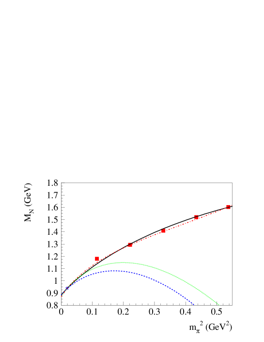
Figure 2: (Color online) Pion-mass dependence of the nucleon mass. The dashed (blue) curve is the leading-nonanalytic $m_{\pi}^{3}$ result, whereas the solid (black) curve is the full relativistic $\pi N$-loop result, both for parameter values: $M_{N}^{(0)}=0.883$ GeV and $c_{1N}=-0.87$ GeV^-1. The dotted (green) curve is the relativistic result for $\pi N+\pi\Delta$ loops with $M_{N}^{(0)}=0.87$ GeV and $c_{1N}=-1.1$ GeV^-1. Upon adding to this result the $m_{\pi}^{4}$ term, Eq. (23), with $c_{2N}=3.0$ GeV^-3, one obtains the dash-dotted (red) curve. The (red) squares are lattice results from the MILC Collaboration Bernard:2001av . The star represents the physical mass value, which is used in the fits.

We are now in position to discuss the numerical results. Fig. 2 displays the pion-mass dependence of the nucleon mass, as given by Eq. (17). The two low-energy constants $M_{N}^{(0)}$ and $c_{1N}$ are related to reproduce the physical nucleon mass at the physical pion mass value. The only free parameter can then be adjusted to reproduce the lattice data, shown by the squares. Note that these lattice data are not corrected for finite volume effects, which are known to increase with decreasing $m_{\pi}$, and have been estimated to reach 0.03 GeV for $m_{\pi}^{2}=0.1$ GeV² Ross05 . The solid curve in Fig. 2 shows the $\pi N$-loop contribution to the nucleon mass, with $M_{N}^{(0)}=0.883$ GeV and $c_{1N}=-0.87$ GeV^-1. Thus, the relativistic calculation is able to describe the lattice results up to $m_{\pi}^{2}\simeq 0.5$ GeV² with only a single free parameter. For comparison, the dashed curve shows the corresponding leading non-analytic result [$m_{\pi}^{3}$ term in Eq. (19)] for the same parameters. One sees that the region of applicability of the leading non-analytic term at this order is considerably smaller, extends up to $m_{\pi}^{2}\simeq 0.05$ GeV². The relativistic result gives a better description out to larger pion-mass values due to a resummation of higher order effects ($m_{\pi}^{4}\ln m_{\pi}$, $m_{\pi}^{5}$, etc., terms), which ensures the correct analyticity properties. The pion-nucleon sigma-term can be obtained in this calculation as $\sigma_{N}=m_{\pi}^{2}\,dM_{N}/dm_{\pi}^{2}$, taken at physical $m_{\pi}$:

$$\sigma_{N}=67-17=50\,\,\left[\mbox{MeV}\right],$$ (21)

where the first number refers to the contribution of the low-energy constant $c_{1N}$, while the second is the chiral loop correction.

The dotted curve in Fig. 2 shows the relativistic result for both $\pi N$ and $\pi\Delta$ loops according to Eq. (17), with slightly re-adjusted low energy constants $M_{N}^{(0)}=0.870$ GeV, $c_{1N}=-1.1$ GeV^-1. One sees that the $\pi\Delta$ loop gives a substantial contribution for larger pion masses and spoils the agreement of our $p^{3}$ relativistic calculation with lattice data, above $m_{\pi}^{2}\simeq 0.15$ GeV². The corresponding sigma-term is

$$\sigma_{N}=85-17-11=57\,\,\left[\mbox{MeV}\right],$$ (22)

where the numbers refer to the contributions of $c_{1N}$, the $\pi N$, and the $\pi\Delta$ loops, respectively.

In absence of a complete fourth order calculation for both $\pi N$ and $\pi\Delta$ loop contributions, we estimate the higher order terms here in a simple way by allowing for one additional term, proportional to $m_{\pi}^{4}$ in the baryon mass formula as :

$$M_{B}=M_{B}^{(0)}-4\,c_{1B}\,m_{\pi}^{2}+c_{2B}\,m_{\pi}^{4}+\,\mbox{chiral loops},$$ (23)

where the chiral loop contribution is calculated as discussed above in Eq. (17). Such a procedure was also proposed before in Ref. Ross05 , when applying a heavy-baryon formula for the non-analytic contribution in the quark mass to lattice results. We see from Fig. 2, that with this 3 parameter formula, one can obtain a description of the lattice calculation with the relativistic $\pi N+\pi\Delta$ result up to $m_{\pi}^{2}\simeq 0.5$ GeV², using as parameter values : $M_{N}^{(0)}=0.87$ GeV, $c_{1N}=-1.1$ GeV^-1, and $c_{2N}=3.0$ GeV^-3. Although the $m_{\pi}^{4}$ term only contributes about 1 MeV to the nucleon mass for physical pion mass values, its contribution at $m_{\pi}^{2}=0.5$ GeV² amounts to about 750 MeV. We notice that in Ref. Ross05 the value of the coefficient $c_{2N}$ was also found to be large, which signals the importance of further higher-order terms.

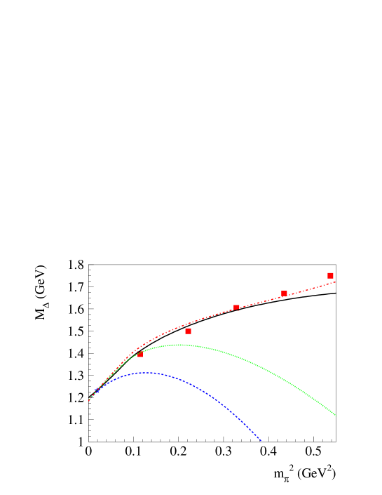
Figure 3: (Color online) Pion-mass dependence of the $\Delta$ mass. The solid (black) curve is the relativistic $\pi N$ loop result, with $M_{\Delta}^{(0)}=1.20$ GeV and $c_{1\Delta}=-0.40$ GeV^-1. The dashed (blue) curve is the leading non-analytic $m_{\pi}^{3}$ result (arising from $\pi\Delta$ loops), with $M_{\Delta}^{(0)}=1.185$ GeV and $c_{1\Delta}=-0.75$ GeV^-1. The dotted (green) curve shows the relativistic $\pi N+\pi\Delta$ result for the same parameters, whereas upon adding to this result the $m_{\pi}^{4}$ term as in Eq. (23), with $c_{2\Delta}=2.0$ GeV^-3, one obtains the dash-dotted (red) curve. The (red) squares are lattice results from the MILC Collaboration Bernard:2001av . The star represents the physical mass value, which is used in the fits.

Fig. 3 displays the results for the $\Delta$ mass. As in the nucleon case, the relativistic $\pi N$ loop result, shown by the solid curve, is able to provide a surprisingly good description of the lattice results up to about $m_{\pi}^{2}\simeq 0.4$ GeV², using $M_{\Delta}^{(0)}=1.20$ GeV, $c_{1\Delta}=-0.40$ GeV^-1. When including the $\pi\Delta$ loops one notices that although the convergence of the relativistic calculation (dotted curve in Fig. 3) is improved in comparison with the leading-nonanalytic result (dashed curve in Fig. 3), its agreement with the lattice results is limited to $m_{\pi}^{2}\simeq 0.1$ GeV².

As for the nucleon, we estimate remaining fourth order contributions by the form of Eq. (23). Using such a three parameter form, the relativistic $\pi N+\pi\Delta$ loop calculation is able to describe the pion mass dependence of the $\Delta$ mass up to $m_{\pi}^{2}\simeq 0.5$ GeV², with $M_{\Delta}^{(0)}=1.185$ GeV, $c_{1\Delta}=-0.75$ GeV^-1, and $c_{2\Delta}=2$ GeV^-3. We note that the coefficient $c_{2\Delta}$ is of the same size as for the nucleon and represents a 500 MeV mass contribution to the $\Delta$ mass at $m_{\pi}^{2}=0.5$ GeV².

In conclusion, we have studied the pion-mass dependence of nucleon and $\Delta$-isobar masses within the framework of a manifestly covariant chiral effective-field theory. We have computed the one-loop $\pi N$ and $\pi\Delta$ graphs and obtained a generic expression for those contributions to the masses and field renormalization constants, Eq. (17). We were able to obtain these generic expressions because of a specific choice of the chiral Lagrangian, where the $\pi N\Delta$ and $\pi\Delta\Delta$ couplings are constructed to be consistent with the spin degrees of freedom counting of the relativistic spin-3/2 field. For the $\pi NN$ coupling we adopt a form which is similar to the above-mentioned $\Delta$ couplings. The resulting relativistic loop corrections obey the chiral power-counting, after renormalizations of the available counter-terms are done. The relativistic expressions also contain the nominally higher-order terms, which are necessary to satisfy the analyticity constraint. As has been shown here on the example of the nucleon and $\Delta$ masses, the convergence of the chiral expansion can be improved in this way, without introducing additional free parameters. In particular, we find that the relativistic calculation, including only the $\pi N$ loops, is able to describe the lattice results for both nucleon and $\Delta$ masses up to $m_{\pi}^{2}\simeq 0.5$ GeV² with only one free parameter. Including the $\pi\Delta$ loops, however, spoils the agreement with the lattice result. We then estimated the effect of the higher-order terms by adding a $m_{\pi}^{4}$ term to the baryon mass. Using the additional free parameter, one is able to obtain a description of the lattice calculation with the relativistic $\pi N+\pi\Delta$ result up to $m_{\pi}^{2}\simeq 0.5$ GeV². While a full fourth order calculation of both $\pi N$ and $\pi\Delta$ loops is a worthwhile topic for future work, the present relativistic chiral-loop calculation can be used in the interpolation between full lattice QCD simulations and the experimental results.

Appendix A Conventions, rules and identities

Here we summarize the conventions, Feynman rules, and list a few useful identities used throughout this work.

• Conventions: $g^{\mu\nu}=\mbox{diag}(1,-1,-1,-1)$, $\varepsilon^{0123}=1$, $\gamma_{5}=i\gamma_{0}\gamma_{1}\gamma_{2}\gamma_{3}$, $(\gamma^{\mu})^{\dagger}=\gamma^{0}\gamma^{\mu}\gamma^{0}$, $\gamma_{5}^{\dagger}=\gamma_{5}$. Furthermore, $\gamma$’s denote Dirac’s $\gamma$-matrices and their totally-antisymmetric products: $\gamma^{\mu\nu}=\mbox{\small{$\frac{1}{2}$}}[\gamma^{\mu},\gamma^{\nu}]$, $\gamma^{\mu\nu\alpha}=\mbox{\small{$\frac{1}{2}$}}\{\gamma^{\mu\nu},\gamma^{\alpha}\}$, $\gamma^{\mu\nu\alpha\beta}=\mbox{\small{$\frac{1}{2}$}}[\gamma^{\mu\nu\alpha},\gamma^{\beta}]$.

• Propagators:

  $$S_{\pi}(p) = (p^{2}-m_{\pi}^{2}+i\varepsilon)^{-1},$$ (24a)

  $$S_{N}(p) = (p/-M_{N}+i\varepsilon)^{-1}=(p/+M_{N})\,(p^{2}-M_{N}^{2}+i\varepsilon)^{-1},$$ (24b)

  $$S_{\Delta}^{\alpha\beta}(p) = -(p/+M_{\Delta})\,(p^{2}-M_{\Delta}^{2}+i\varepsilon)^{-1}\,{\mathscr{P}}^{(3/2)\alpha\beta}(p).$$ (24c)

• Vertices:

  $${\it\Gamma}_{\pi NN}^{(1)a}(p^{\prime},p) = \frac{g_{A}}{2M_{N}f_{\pi}}i\varepsilon^{\alpha\beta\varrho\sigma}\gamma_{\alpha}\gamma_{\beta}p_{\varrho}p_{\sigma}^{\prime}\,\tau^{a},$$ (25a)

  $${\it\Gamma}_{\pi N\Delta}^{(1)a,\,\alpha}(p^{\prime},p) = \frac{h_{A}}{2M_{\Delta}f_{\pi}}i\varepsilon^{\alpha\beta\varrho\sigma}p_{\beta}^{\prime}p_{\varrho}\gamma_{\sigma}\,\gamma_{5}T^{a},$$ (25b)

  $${\it\Gamma}_{\pi\Delta\Delta}^{(1)a,\,\alpha\beta}(p^{\prime},p) = \frac{H_{A}}{2M_{\Delta}f_{\pi}}i\varepsilon^{\alpha\beta\varrho\sigma}p_{\varrho}p_{\sigma}^{\prime}\,{\cal T}^{a}\,.$$ (25c)

• Identities:

  $$i\varepsilon^{\mu\nu\varrho\sigma}\gamma_{\sigma}\gamma_{5}=\gamma^{\mu\nu\varrho}=\mbox{\small{$\frac{1}{2}$}}(\gamma^{\mu}\gamma^{\nu}\gamma^{\varrho}-\gamma^{\varrho}\gamma^{\nu}\gamma^{\mu}),$$ (26a)

  $$i\varepsilon^{\mu\nu\varrho\sigma}\gamma_{5}=\gamma^{\mu\nu\varrho\sigma}=\mbox{\small{$\frac{1}{4}$}}(\gamma^{\mu}\gamma^{\nu}\gamma^{\varrho}\gamma^{\sigma}-\gamma^{\varrho}\gamma^{\nu}\gamma^{\mu}\gamma^{\sigma}+\gamma^{\mu}\gamma^{\varrho}\gamma^{\nu}\gamma^{\sigma}-\gamma^{\nu}\gamma^{\sigma}\gamma^{\mu}\gamma^{\varrho})\,,$$ (26b)

  $$\varepsilon^{\mu}_{\,\lambda\sigma\alpha}\,p^{\lambda}\,\gamma^{\sigma}\,\varepsilon_{\mu\nu\rho\beta}\,p^{\nu}\,\gamma^{\rho}=-p^{2}({\rm g}_{\alpha\beta}+\gamma_{\alpha}\gamma_{\beta})+p/\gamma_{\beta}p_{\alpha}+\gamma_{\alpha}p_{\beta}p/,$$ (26c)

  $$\varepsilon_{\mu\lambda\sigma\alpha}\,p^{\lambda}\,\gamma^{\sigma}\left({\rm g}^{\mu\mu^{\prime}}-\mbox{\small{$\frac{1}{3}$}}\gamma^{\mu}\gamma^{\mu^{\prime}}\right)\,\varepsilon_{\mu^{\prime}\nu\rho\beta}\,p^{\nu}\,\gamma^{\rho}=-p^{2}\,{\mathscr{P}}^{3/2}_{\alpha\beta}(p),$$ (26d)

  $$\varepsilon^{\alpha\mu\varrho^{\prime}\sigma^{\prime}}p_{\varrho^{\prime}}k_{\sigma^{\prime}}\,\varepsilon^{\beta\nu\varrho\sigma}p_{\varrho}k_{\sigma}\,\,g_{\mu\nu}=-g^{\alpha\beta}[p^{2}k^{2}-(p\cdot k)^{2}]+p^{\alpha}p^{\beta}k^{2}+k^{\alpha}k^{\beta}p^{2}$$

  $$\hskip 142.26378pt-\,p\cdot k\,(p^{\alpha}k^{\beta}+p^{\beta}k^{\alpha})\,,$$ (26e)

  $$\varepsilon^{\alpha\mu\varrho^{\prime}\sigma^{\prime}}p_{\varrho^{\prime}}k_{\sigma^{\prime}}\,\gamma_{\mu}\,\gamma_{\nu}\,\varepsilon^{\beta\nu\varrho\sigma}p_{\varrho}k_{\sigma}\,{\mathscr{P}}^{3/2}_{\alpha\beta}(p)=-p^{2}\,k^{\alpha}k^{\beta}\,{\mathscr{P}}^{3/2}_{\alpha\beta}(p).$$ (26f)

Appendix B Relativistic loop functions

Here we explicitly define functions $\overline{V}$ and $\overline{W}$ which enter the mass and FRC correction formula (17).

$$\overline{V}(\mu,\delta) \equiv V(\mu,\delta)-V(0,\delta)-V^{\prime}(0,\delta)\mu^{2}\,,$$ (27a)

$$V(\mu,\delta) = \int_{0}^{1}\!dx\,(R+x)\,\left\{\mu^{2}x+(1-x)(R^{2}-x)\right\}\,\ln\{\mu^{2}x+(1-x)(R^{2}-x)\}$$

$$= \mbox{\small{$\frac{1}{3}$}}(R+\alpha)\left[\beta\,(\mu^{2}-2\lambda^{2})\,\ln\mu^{2}+\alpha\,(R^{2}-2\lambda^{2})\,\ln R^{2}-\mbox{$\frac{2}{3}$}(\alpha^{3}+\beta^{3})\right.$$

$$+ \left.4\lambda^{2}+4\lambda^{4}\,\Omega(\lambda)\,\right]+\mbox{\small{$\frac{1}{4}$}}\mu^{4}(\ln\mu^{2}-\mbox{\small{$\frac{1}{2}$}})-\mbox{\small{$\frac{1}{4}$}}R^{4}(\ln R^{2}-\mbox{\small{$\frac{1}{2}$}})\,,$$

$$V(0,\delta) = \mbox{$\frac{5}{36}$}+\mbox{$\frac{5}{18}$}R-\mbox{$\frac{7}{36}$}R^{2}-\mbox{$\frac{2}{3}$}R^{3}-\mbox{$\frac{1}{8}$}R^{4}+\mbox{$\frac{1}{6}$}R^{5}+\mbox{$\frac{1}{12}$}R^{6}$$

$$- \mbox{$\frac{1}{6}$}R^{5}(R^{3}+2R^{2}-2R-6)\,\ln R+\mbox{$\frac{1}{12}$}(R^{2}-1)^{3}(1+R)^{2}\,\ln|R^{2}-1|\,,$$

$$V^{\prime}(0,\delta) \equiv \left.({\partial}/{\partial\mu^{2}})V(\mu,\delta)\right|_{\mu=0}=-\mbox{$\frac{1}{18}$}(7+9R+3R^{2}+9R^{3}+6R^{4})$$ (27d)

$$+ \mbox{\small{$\frac{1}{3}$}}R^{5}(3+2R)\,\ln R+\mbox{\small{$\frac{1}{3}$}}(1+\mbox{\small{$\frac{3}{2}$}}R-\mbox{\small{$\frac{3}{2}$}}R^{5}-R^{6})\,\ln|R^{2}-1|\,,$$

where $R\equiv 1+\delta$, $\beta=-\delta-\mbox{\small{$\frac{1}{2}$}}(\delta^{2}-\mu^{2})=\mbox{\small{$\frac{1}{2}$}}(1-R^{2}+\mu^{2})$, $\alpha=1-\beta$, $\lambda^{2}=\mbox{\small{$\frac{1}{4}$}}[\delta^{2}-\mu^{2}][(2+\delta)^{2}-\mu^{2}]$, and the elementary function $\Omega$ is defined as:

$$\Omega(\lambda)=\left\{\begin{array}[]{lc}\frac{1}{2\lambda}\ln\mbox{$\frac{\beta-\mu^{2}-\lambda}{\beta-\mu^{2}+\lambda}$}\,,&\lambda^{2}\geq 0\\ -\frac{1}{\sqrt{-\lambda^{2}}}\arctan\frac{\sqrt{-\lambda^{2}}}{\alpha\beta+\lambda^{2}}\,,&\lambda^{2}<0\,.\end{array}\right.$$ (28)

Similarly,

$$\overline{W}(\mu,\delta) \equiv W(\mu,\delta)-W(0,\delta)-W^{\prime}(0,\delta)\mu^{2}\,,$$ (29a)

$$W(\mu,\delta) = \int_{0}^{1}\!dx\,x\,\left\{\mu^{2}x+(1-x)(R^{2}-x)\right\}\,\ln\{\mu^{2}x+(1-x)(R^{2}-x)\}$$

$$= \mbox{\small{$\frac{1}{3}$}}\alpha\left[\beta\,(\mu^{2}-2\lambda^{2})\,\ln\mu^{2}+\alpha\,(R^{2}-2\lambda^{2})\,\ln R^{2}-\mbox{$\frac{2}{3}$}(\alpha^{3}+\beta^{3})\right.$$

$$+ \left.4\lambda^{2}+4\lambda^{4}\,\Omega(\lambda)\,\right]+\mbox{\small{$\frac{1}{4}$}}\mu^{4}(\ln\mu^{2}-\mbox{\small{$\frac{1}{2}$}})-\mbox{\small{$\frac{1}{4}$}}R^{4}(\ln R^{2}-\mbox{\small{$\frac{1}{2}$}}),$$

$$W(0,\delta) = \mbox{$\frac{5}{36}$}-\mbox{$\frac{7}{36}$}R^{2}-\mbox{$\frac{1}{8}$}R^{4}+\mbox{$\frac{1}{12}$}R^{6}$$ (29c)

$$- \mbox{$\frac{1}{6}$}R^{6}(R^{2}-2R)\,\ln R+\mbox{$\frac{1}{12}$}(R^{2}-1)^{3}(1+R^{2})\,\ln|R^{2}-1|\,,$$

$$W^{\prime}(0,\delta) \equiv \left.({\partial}/{\partial\mu^{2}})W(\mu,\delta)\right|_{\mu=0}=-\mbox{$\frac{1}{18}$}(7+3R^{2}+6R^{4})$$ (29d)

$$+ \mbox{$\frac{2}{3}$}R^{6}\,\ln R+\mbox{\small{$\frac{1}{3}$}}(1-R^{6})\,\ln|R^{2}-1|\,,$$

It is useful to know the expansion of these functions for small $\mu$:

$$\overline{V}(\mu,\delta) = \frac{\mu^{4}}{\delta}\left[-\ln\mu+\mbox{\small{$\frac{1}{4}$}}R\,(1+2R^{2})-R^{5}\ln R+\mbox{\small{$\frac{1}{2}$}}(1+R^{5})\,\ln|R^{2}-1|\right]+O(\mu^{5}),$$ (30a)

$$\overline{W}(\mu,\delta) = \frac{\mu^{4}}{\delta}\frac{[-\ln\mu+\mbox{\small{$\frac{1}{4}$}}R^{2}(1+2R^{2})-R^{6}\ln R+\mbox{\small{$\frac{1}{2}$}}(1+R^{6})\,\ln|R^{2}-1|]}{1+R}+O(\mu^{5}).$$ (30b)

For $\delta=0$, the expansion takes a different form:

$$\overline{V}(\mu,0) = \frac{4\pi}{3}\mu^{3}+\frac{5}{2}\mu^{4}\left(-\mbox{\small{$\frac{1}{4}$}}+\ln\mu\right)+O(\mu^{5}),$$ (31a)

$$\overline{W}(\mu,0) = \frac{2\pi}{3}\mu^{3}+\frac{3}{2}\mu^{4}\left(-\mbox{$\frac{1}{12}$}+\ln\mu\right)+O(\mu^{5}).$$ (31b)

References

• (1) For a review, see D. B. Leinweber, W. Melnitchouk, D. G. Richards, A. G. Williams and J. M. Zanotti, Lect. Notes Phys.  663, 71 (2005); C. DeTar and S. Gottlieb, Phys. Today 57N2, 45 (2004).
• (2) C. W. Bernard et al. [MILC Collaboration], Phys. Rev. D 64, 054506 (2001); ibid. 70, 094505 (2004).
• (3) D. B. Leinweber, A. W. Thomas and R. D. Young, Phys. Rev. Lett.  86, 5011 (2001); W. Detmold, W. Melnitchouk, J. W. Negele, D. B. Renner and A. W. Thomas, ibid.  87, 172001 (2001).
• (4) T. R. Hemmert, M. Procura and W. Weise, Phys. Rev. D 68, 075009 (2003).
• (5) V. Pascalutsa and M. Vanderhaeghen, Phys. Rev. Lett. 95 (in press) [arXiv:hep-ph/0508060].
• (6) M. K. Banerjee and J. Milana, Phys. Rev. D 52, 6451 (1995).
• (7) A. W. Thomas and G. Krein, Phys. Lett. B 456, 5 (1999).
• (8) D. B. Leinweber, A. W. Thomas, K. Tsushima and S. V. Wright, Phys. Rev. D 61, 074502 (2000).
• (9) R. D. Young, D. B. Leinweber, A. W. Thomas and S. V. Wright, Phys. Rev. D 66, 094507 (2002); R. D. Young, D. B. Leinweber and A. W. Thomas, Prog. Part. Nucl. Phys.  50, 399 (2003); D. B. Leinweber, A. W. Thomas and R. D. Young, Phys. Rev. Lett.  92, 242002 (2004).
• (10) V. Bernard, T. R. Hemmert and U. G. Meissner, Phys. Lett. B 565, 137 (2003); ibid. 622, 141 (2005).
• (11) C. Hacker, N. Wies, J. Gegelia and S. Scherer, arXiv:hep-ph/0505043.
• (12) M. Luscher, Plenary talk at 23rd International Symposium on Lattice Field Field: Lattice 2005, Trinity College, Dublin, Ireland, (July 2005) [arXiv:hep-lat/0509152].
• (13) T. Becher and H. Leutwyler, Eur. Phys. J. C 9, 643 (1999).
• (14) T. Fuchs, J. Gegelia, G. Japaridze and S. Scherer, Phys. Rev. D 68, 056005 (2003).
• (15) B. R. Holstein, V. Pascalutsa and M. Vanderhaeghen, Phys. Rev. D 72, 094014 (2005); Phys. Lett. B 600, 239 (2004); V. Pascalutsa, Prog. Part. Nucl. Phys.  55, 23 (2005).
• (16) J. Gasser, M. E. Sainio and A. Svarc, Nucl. Phys. B 307, 779 (1988).
• (17) E. Jenkins and A. V. Manohar, Phys. Lett. B 255, 558 (1991).
• (18) J. Gegelia, G. Japaridze and X. Q. Wang, J. Phys. G 29, 2303 (2003) [arXiv:hep-ph/9910260].
• (19) W. Rarita and J. S. Schwinger, Phys. Rev.  60, 61 (1941).
• (20) V. Pascalutsa, Phys. Rev. D 58, 096002 (1998); V. Pascalutsa and R. Timmermans, Phys. Rev. C 60, 042201(R) (1999).
• (21) V. Pascalutsa, Phys. Lett. B 503, 85 (2001).
• (22) V. Pascalutsa, PhD Thesis (University of Utrecht, 1998) [Hadronic J. Suppl.  16, 1 (2001)], Ch. 3.
• (23) C. L. Korpa and A. E. L. Dieperink, Phys. Rev. C 70, 015207 (2004).
• (24) A. E. Kaloshin and V. P. Lomov, arXiv:hep-ph/0409052; Mod. Phys. Lett. A 19, 135 (2004).
• (25) T. D. Cohen and W. Broniowski, Phys. Lett. B 292, 5 (1992).
• (26) V. Pascalutsa and D. R. Phillips, Phys. Rev. C 67, 055202 (2003).
• (27) V. Pascalutsa and M. Vanderhaeghen, Phys. Rev. Lett.  94, 102003 (2005).