Final State Interaction In $B\to KK$ Decays

Abstract

We study the final state interaction effects in $B\to KK$ decays. We find that the $t$ channel one-particle-exchange diagrams cannot enhance the branching ratios of $\overline{B}^{0}\to K^{0}\overline{K^{0}}$ and $B^{-}\to K^{0}K^{-}$ very sizably. For the pure annihilation process $\overline{B}^{0}\to K^{+}K^{-}$, the obtained branching ratio by final state interaction is at ${\cal{O}}(10^{-8})$.

I Introduction

$B$ meson non-leptonic decays are important to study CP violation and to extract CKM parameters. When the $B$ meson decays into two light mesons, the final state particles are energetic, so it is argued that they do not have enough time to get involved in soft final state interaction(FSI). In spite of the FSI, several factorization approaches, such as the naive factorization approach (FA) fac ; akl1 ; chengfac , the QCD factorization approach (QCDF) bene , the perturbative QCD approach (PQCD) kls ; lucd and Soft-Collinear-Effective-Theory (SCET) scet have been established to analyze $B$ meson decays. These approaches successfully explain many phenomenons, but there are still some problems hard to explain within these frameworks, which have been summarized in cheng . These may be hints of the need of FSI in $B$ decays. It has been argued that the FSI is power suppressed for the cancellation of the various intermediate states in the heavy quark limit bene , but for the finite bottom quark mass, this effect may not be very effective buras . So FSI may be important to the channels that are suppressed by other factors (such as the color factor or the CKM matrix elements). For example, $B\to KK$ decays are usually considered to be in the category lhn .

FSI effects are nonperturbative in nature, so it is difficult to study in a systematic way and some different mechanism of the rescattering effects have been considered. In the study of $D$ meson decays, the form factors are introduced to parameterize the offshellness of the exchanged particles form1 ; form2 , and this method still works in $B$ meson case. This mechanism has been used to explain some puzzles cheng ; cheng2 , such as $B\to\pi\pi,\pi K$ puzzle, it is argued that these puzzles can be resolved by FSI if we adopt appropriate parameters. If this is the right method to resolve these puzzles, it should be consistent with other channels, such as the small branching ratio of $B\to KK$ and $B\to\rho^{0}\rho^{0}$ decays. The $B\to KK$ decays have been measured by Belle belle and Babar babar , which are shown in TABLE 1( where the world average values are taken from hfag ). The FA predictions can be consistent with the experiment for $B^{0}\to K^{0}\overline{K}^{0}$ and $B^{+}\to\overline{K}^{0}K^{+}$ if we employ the current nonperturbative inputs akl1 ; bene , thus the FSI effects may not be too large. The $\overline{B}^{0}\to K^{+}{K^{-}}$ is a pure annihilation decay channel, so it is expected to be very small in FA, and the FSI can give sizable corrections. In this paper we will follow the method in cheng , focusing on the two body intermediate states and considering only $t$-channel one-particle-exchange processes at hadron level. We will give the detailed calculation of the FSI effects for $B\to KK$ decays in the next section, and then a brief summary in the third section.

TABLE.1.  Measured branching fractions ($$\times 10^{-6}$$) of decays

Channel Babar Belle World average

II Final State Interactions Effects In $B\to KK$ Decays

Before analyzing the FSI in $B\to KK$ decays, we first explore what we can get in the usual short distance analysis. The short distance contribution of the heavy meson decays can be expressed in terms of some types of quark diagrams: ${\cal P}$, the penguin emission diagram; ${\cal E}$, W-exchange diagram; ${\cal A}$, $W$-annihilation diagram; ${\cal P}_{A}$, the penguin annihilation diagram (space-like); ${\cal P}_{EW}$, the electroweak penguin diagram; ${\cal V}$, the vertical $W$ loop diagram (time-like penguin). The penguin dominated $B\to KK$ decays can be expressed as:

$$A(\overline{B}^{0}\to K^{0}\overline{K^{0}})={\cal P}+{\cal P}_{A}-\frac{1}{3}{\cal P}_{EW}+{\cal V},$$

$$A(B^{-}\to K^{0}K^{-})={\cal P}+{\cal P}_{A}-\frac{1}{3}{\cal P}_{EW}+{\cal A},$$

$$A(\overline{B}^{0}\to K^{+}K^{-})={\cal E}+{\cal V}.$$ (1)

In factorization approach, there is no emission tree diagram contribution to these decays. The annihilation diagrams ${\cal A},{\cal E},{\cal V},{\cal P}_{A}$ are power suppressed which can be neglected in the calculation. They are usually believed to be long distance dominant. So the short distance amplitudes read:

$$A(\overline{B}^{0}\to K^{0}\overline{K^{0}}) =i\frac{G_{F}}{\sqrt{2}}f_{K}F_{0}^{BK}(m_{K}^{2})(m_{B}^{2}-m_{K}^{2})[V_{ub}V_{ud}^{*}(a_{4}^{u}+r^{K}_{\chi}a_{6}^{u})+V_{cb}V_{cd}^{*}(a_{4}^{c}+r^{K}_{\chi}a_{6}^{c})$$ (2)

$$+V_{ub}V_{ud}^{*}(a_{10}^{u}+r^{K}_{\chi}a_{8}^{u})+V_{cb}V_{cd}^{*}(a_{10}^{c}+r^{K}_{\chi}a_{8}^{c})],$$

and $A(B^{-}\to K^{0}K^{-})=A(\overline{B}^{0}\to K^{0}\overline{K^{0}})$ , $A(\overline{B}^{0}\to K^{+}K^{-})=0$, where $V_{ub},V_{ud},V_{cb}$ and $V_{cd}$ are CKM matrix elments, $r^{K}_{\chi}=2m_{K}^{2}/[m_{b}(m_{s}+m_{q})]$. $a_{i}^{u,c}$ are combination of Wilson coefficients for four quark operators defined in in ref.akl1 .

$$a_{i}=C_{i}+\frac{1}{3}C_{i+1},\,\,(i=odd)$$

$$a_{i}=C_{i}+\frac{1}{3}C_{i-1},\,\,(i=even)$$ (3)

From quark-hadron duality, the decay amplitude can be got from either quark picture or hadron picture. The result should be equal. However, neither of the two pictures are fully understood in the B decays. The factorization theorem tells us to calculate the short distance contribution perturbatively and the long distance parts using hadronic picture. Thus a double counting problem may arise. To avoid double counting, we adopt leading order Wilson coefficient at the scale $m_{b}$ for naive factorization approach instead of QCDF (which includes some virtual corrections from long distance) for short distance calculations of $B\to KK$.

When we calculate the long distance contributions to the decays, we consider only the CKM most favored two body intermediate states, such as $D^{(*)}D^{(*)},\pi\pi,\rho\rho$. The quark level $B\to\pi\pi(\rho\rho)\to KK$ diagrams are shown in Figure 1. We can see that the this diagram has the same topology as the penguin diagram or $W$-exchange diagram. From Eq.(1), we can see that this kind of diagrams can contribute to $B\to K^{0}\overline{K^{0}},K^{+}K^{-},K^{0}K^{-}$ simultaneously. When the intermediate state is $D^{(*)+}D^{(*)-}(D^{(*)+}\bar{D}^{(*)0})$, only penguin topology works, so it cannot contribute to the $\overline{B}^{0}\to K^{+}K^{-}$ decay.

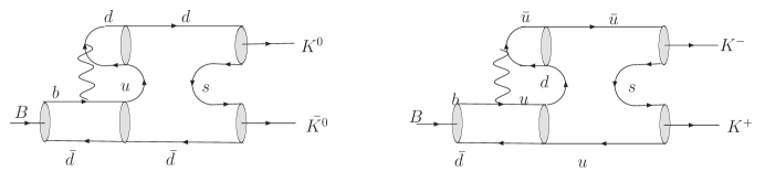
Figure 1: Quark level diagram for $B\to\pi^{+}\pi^{-}\to K^{0}\overline{K^{0}}(K^{+}K^{-})$

The hadron level diagrams are given in Figure 2. We focus on the $t$ channel one-particle-exchange processes, furthermore, we consider only the case that the two intermediate particles are on shell, i.e. we only keep the absorptive part of diagrams in Figure 2, which gives the main contribution.

Figure 2: Hadron level diagrams for long distance $t$ channel contribution to $B\to KK$

The absorptive part of the diagrams in Figure 2 can be calculated with the following formula:

$${\cal A}bs\,A(P_{B}\to p_{3}p_{4})= {1\over 2}\int{d^{3}p_{1}\over(2\pi)^{3}2E_{1}}\,{d^{3}p_{2}\over(2\pi)^{3}2E_{2}}\,(2\pi)^{4}\delta^{4}(p_{3}+p_{4}-p_{1}-p_{2})A(P_{B}\to p_{1}p_{2})$$

$$\times T^{*}(p_{3}p_{4}\to p_{1}p_{2}),$$ (4)

which can be deduced using the optical theorem cheng .

Taken FSI corrections into account, the topological amplitudes are:

$${\cal P}={\cal P}_{SD}+i{\cal A}bs(a+b+c+d),$$

$${\cal E}=i{\cal A}bs(a+b).$$ (5)

Then the decay amplitudes turn to:

$$A(\overline{B}^{0}\to K^{0}\overline{K^{0}})={\cal P}+{\cal P}_{EW}+i{\cal A}bs(a+b+c+d),$$

$$A(B^{-}\to K^{0}K^{-})={\cal P}+{\cal P}_{EW}+i{\cal A}bs(a+b+c+d),$$

$$A(\overline{B}^{0}\to K^{+}K^{-})=i{\cal A}bs(a+b).$$ (6)

To perform the calculation, we introduce the relevant Lagrangian density Casalbuoni :

$${\cal L}_{l} = -{1\over 4}Tr[F_{\mu\nu}(V)F^{\mu\nu}(V)]+ig_{VPP}Tr(V^{\mu}P\buildrel\leftrightarrow\over{\partial}_{\mu}P)+g_{VVP}\epsilon^{\mu\nu\alpha\beta}Tr(\partial_{\mu}V_{\nu}\partial_{\alpha}V_{\beta}P),$$ (7)

$${\cal L}_{D} = -ig_{D^{*}DP}(D^{i}\partial^{\mu}P_{ij}D^{*j\dagger}_{\mu}-D^{*i}_{\mu}\partial^{\mu}P_{ij}D^{j\dagger})-\frac{1}{2}g_{D^{*}D^{*}P}\epsilon_{\mu\nu\alpha\beta}D_{i}^{*\mu}\partial^{\nu}P^{ij}\buildrel\leftrightarrow\over{\partial^{\alpha}}D_{j}^{*\beta\dagger}$$ (8)

$$-ig_{DDV}D_{i}^{\dagger}\buildrel\leftrightarrow\over{\partial}_{\mu}D^{j}(V^{\mu})^{i}_{j}-2f_{D^{*}DV}\epsilon_{\mu\nu\alpha\beta}(\partial^{\mu}V^{\nu})^{i}_{j}(D_{i}^{\dagger}\buildrel\leftrightarrow\over{\partial^{\alpha}}D^{*\beta j}-D^{*\beta\dagger}_{i}\buildrel\leftrightarrow\over{\partial^{\alpha}}D^{j})$$

$$+ig_{D^{*}D^{*}V}D^{*\nu\dagger}_{i}\buildrel\leftrightarrow\over{\partial}_{\mu}D_{\nu}(V^{\mu})^{i}_{j}+4if_{D^{*}D^{*}V}D^{*\dagger}_{i\mu}(\partial^{\mu}V^{\nu}-\partial^{\nu}V^{\mu})D^{*j}_{\nu},$$

where $P$ and $V_{\mu}$ are pseudoscalar and vector multiplets respectively. Here we take the convention $\epsilon^{0123}=1$.

Using Eq. (4) and the Feynman rules derived from the Eqs. (7) and (8), we can get the leading long distance rescattering amplitude:

$${\cal A}bs(a)=\int_{-1}^{1}\ {|{\bf p}_{1}|d\cos\theta\over 16\pi m_{B}}\,{g^{2}_{K^{*}K\pi}}\,A(\overline{B}^{0}\to\pi^{+}\pi^{-})\,{F^{2}(t,m_{K^{*}})\over{t-m_{K^{*}}^{2}}+im_{K^{*}}\Gamma_{K^{*}}}\,H_{1},$$ (9)

with

$$A(\overline{B}^{0}\to\pi^{+}\pi^{-}) = i\frac{G_{F}}{\sqrt{2}}f_{\pi}F_{0}^{B\pi}(m_{\pi}^{2})(m_{B}^{2}-m_{\pi}^{2})[V_{ub}V_{ud}^{*}(a_{1}+a_{4}^{u}+a_{10}^{u}+r^{\pi}_{\chi}(a_{6}^{u}+a_{8}^{u}))$$

$$+ V_{cb}V_{cd}^{*}(a_{4}^{c}+a_{10}^{c}+r^{\pi}_{\chi}(a_{6}^{c}+a_{8}^{c}))],$$

$$H_{1} = -(p_{1}\cdot p_{2}+p_{3}\cdot p_{4}+p_{1}\cdot p_{4}+p_{2}\cdot p_{3})-{(m_{1}^{2}-m_{3}^{2})(m_{2}^{2}-m_{4}^{2})\over m_{K^{*}}^{2}},$$ (10)

where we denote the momentum by $B(p_{B})\to\pi(p_{1})\pi(p_{2})\to K(p_{3})K(p_{4})$, $\theta$ is the angle between ${\bf p}_{1}$ and ${\bf p}_{3}$, and $r_{\chi}^{\pi}=2m_{\pi}^{2}/[m_{b}(m_{u}+m_{d})]$. Here $F(t,m_{K^{*}})$ is the form factor introduced to denote offshellness of the exchanged particle, which is usually parameterized as cheng :

$$F(t,m)=(\frac{\Lambda^{2}-m^{2}}{\Lambda^{2}-t})^{n}.$$ (11)

It is normalized to unity at $t=m^{2}$ ( $t$ is the invariant mass of the exchanged particle), where we usually take $n=1$. The cutoff $\Lambda$ should not be far from the physical mass of the exchanged particle, where we choose

$$\Lambda=m_{exc}+\eta\Lambda_{QCD}.$$ (12)

The parameter $\eta$ depends not only on exchanged particle, but also on the external particles involved in the strong interaction. If it is determined from the $B\to\pi\pi$ branching ratios, then we can employ it in $B\to KK$ decays for $SU(3)$ symmetry.

Likewise, the absorptive parts of the other diagrams are given by

$${\cal A}bs(b(K)) = -i{{G_{F}}\over{\sqrt{2}}}\,V_{ub}V_{ud}^{*}\int_{-1}^{1}\ {|{\bf p}_{1}|d\cos\theta\over 16\pi m_{B}}\,4g_{\rho KK}^{2}\,{F^{2}(t,m_{K})\over t-m_{K}^{2}}\,$$

$$\times f_{\rho}m_{\rho}\,\Big{[}(m_{B}+m_{\rho})A_{1}^{B\rho}(m_{\rho}^{2})H_{2}-{2A_{2}^{B\rho}(m_{\rho}^{2})\over(m_{B}+m_{\rho})}H^{\prime}_{2}\Big{]},$$

$${\cal A}bs(b(K^{*})) = i{G_{F}\over{\sqrt{2}}}\,V_{ub}V_{ud}^{*}\int_{-1}^{1}{|{\bf p}_{1}|d\cos\theta\over 16\pi m_{B}}\,g_{\rho K^{*}K}^{2}\,{F^{2}(t,m_{K^{*}})\over t-m^{2}_{K^{*}}+im_{K^{*}}\Gamma_{K^{*}}}\,$$

$$\times f_{\rho}m_{\rho}\,\Big{[}(m_{B}+m_{\rho})A_{1}^{B\rho}(m_{\rho}^{2})H_{3}-{2A_{2}^{B\rho}(m_{\rho}^{2})\over(m_{B}+m_{\rho})}H^{\prime}_{3}\Big{]},$$

$${\cal A}bs(c) = \int_{-1}^{1}\ {|{\bf p}_{1}|d\cos\theta\over 16\pi m_{B}}\,{g^{2}_{D^{*}_{s}DK}}\,A(\overline{B}^{0}\to D^{+}D^{-})\,{F^{2}(t,m_{D^{*}_{s}})\over{t-m_{D^{*}_{s}}^{2}}}\,H_{4},$$

$${\cal A}bs(d(D_{s})) = -i{G_{F}\over\sqrt{2}}V_{cb}V_{cd}^{*}\int_{-1}^{1}\frac{|{\bf p}_{1}|d\cos\theta}{16\pi m_{B}}{g^{2}_{D_{s}D^{*}K}}\frac{F^{2}(t,m_{D_{s}})}{t-m_{D_{s}}^{2}}\,$$

$$\times f_{D^{*}}m_{D^{*}}\Big{[}(m_{B}+m_{D^{*}})A_{1}^{BD^{*}}(m_{D^{*}}^{2})H_{5}-\frac{2A_{2}^{BD^{*}}(m_{D^{*}}^{2})}{m_{B}+m_{D^{*}}}H^{\prime}_{5}\Big{]},$$

$${\cal A}bs(d(D_{s}^{*})) = i\frac{G_{F}}{\sqrt{2}}V_{cb}V_{cd}^{*}\int_{-1}^{1}{|{\bf p}_{1}|d\cos\theta\over 16\pi m_{B}}g^{2}_{D_{s}^{*}D^{*}K}\frac{F^{2}(t,m_{D^{*}_{s}})}{t-m_{D^{*}_{s}}^{2}}$$ (13)

$$\times f_{D^{*}}m_{D^{*}}\Big{[}(m_{B}+m_{D^{*}})A_{1}^{BD^{*}}(m_{D^{*}}^{2})H_{6}-\frac{2A_{2}^{BD^{*}}(m_{D^{*}}^{2})}{m_{B}+m_{D^{*}}}H^{\prime}_{6}\Big{]},$$

where

$$H_{2} = (p_{3}\cdot p_{4})-{p_{1}\cdot p_{3}p_{1}\cdot p_{4}\over m_{1}^{2}}-{p_{2}\cdot p_{3}p_{2}\cdot p_{4}\over m_{2}^{2}}+{p_{1}\cdot p_{2}p_{1}\cdot p_{3}p_{2}\cdot p_{4}\over m_{1}^{2}m_{2}^{2}},$$

$$H^{\prime}_{2} = (p_{3}\cdot p_{B})(p_{4}\cdot p_{B})-{(p_{1}\cdot p_{3})(p_{1}\cdot p_{B})(p_{4}\cdot p_{B})\over m_{1}^{2}}-{(p_{2}\cdot p_{4})(p_{2}\cdot p_{B})(p_{3}\cdot p_{B})\over m_{2}^{2}}$$

$$+{(p_{1}\cdot p_{3})(p_{2}\cdot p_{4})(p_{1}\cdot p_{B})(p_{2}\cdot p_{B})\over{m_{1}^{2}m_{2}^{2}}},$$

$$H_{3} = 2(p_{1}\cdot p_{4})(p_{2}\cdot p_{3})-2(p_{1}\cdot p_{2})(p_{3}\cdot p_{4}),$$

$$H^{\prime}_{3} = m_{B}^{2}[(p_{1}\cdot p_{4})(p_{2}\cdot p_{3})-(p_{1}\cdot p_{2})(p_{3}\cdot p_{4})]+(p_{1}\cdot p_{B})(p_{2}\cdot p_{B})(p_{3}\cdot p_{4})$$

$$-(p_{2}\cdot p_{B})(p_{3}\cdot p_{B})(p_{1}\cdot p_{4})-(p_{1}\cdot p_{B})(p_{4}\cdot p_{B})(p_{2}\cdot p_{3})+(p_{3}\cdot p_{B})(p_{4}\cdot p_{B})(p_{1}\cdot p_{2}),$$

$$H_{4} = -(p_{3}\cdot p_{4})+{(p_{1}\cdot p_{3}-m^{2}_{3})(m^{2}_{4}-p_{2}\cdot p_{4})\over m_{D^{*}}^{2}},$$

$$H_{5} = (p_{3}\cdot p_{4})-{(p_{1}\cdot p_{3})(p_{1}\cdot p_{4})\over m_{1}^{2}}-{(p_{2}\cdot p_{3})(p_{2}\cdot p_{4})\over m_{2}^{2}}+{(p_{1}\cdot p_{3})(p_{2}\cdot p_{4})(p_{1}\cdot p_{2})\over{m_{1}^{2}m_{2}^{2}}},$$

$$H^{\prime}_{5} = (p_{3}\cdot p_{B})(p_{4}\cdot p_{B})-{(p_{1}\cdot p_{B})(p_{4}\cdot p_{B})(p_{1}\cdot p_{3})\over m^{2}_{1}}$$

$$-{(p_{2}\cdot p_{B})(p_{3}\cdot p_{B})(p_{2}\cdot p_{4})\over m^{2}_{1}}+{(p_{1}\cdot p_{B})(p_{2}\cdot p_{B})(p_{1}\cdot p_{3})(p_{2}\cdot p_{4})\over{m^{2}_{1}m^{2}_{2}}},$$

$$H_{6} = 2(p_{1}\cdot p_{2})(p_{3}\cdot p_{4})-2(p_{1}\cdot p_{4})(p_{2}\cdot p_{3}),$$

$$H^{\prime}_{6} = m^{2}_{B}[(p_{1}\cdot p_{2})(p_{3}\cdot p_{4})-(p_{1}\cdot p_{4})(p_{2}\cdot p_{3})]-(p_{1}\cdot p_{B})(p_{2}\cdot p_{B})(p_{3}\cdot p_{4})$$ (14)

$$+(p_{2}\cdot p_{B})(p_{3}\cdot p_{B})(p_{1}\cdot p_{4})+(p_{1}\cdot p_{B})(p_{4}\cdot p_{B})(p_{2}\cdot p_{3})-(p_{3}\cdot p_{B})(p_{4}\cdot p_{B})(p_{1}\cdot p_{2}).$$

and

$$A(\overline{B}^{0}\to D^{+}D^{-}) = i\frac{G_{F}}{\sqrt{2}}f_{D}F_{0}^{BD}(m_{D}^{2})(m_{B}^{2}-m_{D}^{2})[V_{cb}V_{cd}^{*}(a_{1}+a_{4}^{c}+a_{10}^{c}+m_{D}/m_{B}(a_{6}^{u}+a_{8}^{u}))$$ (15)

$$+ V_{ub}V_{ud}^{*}(a_{4}^{u}+a_{10}^{u}+m_{D}/m_{B}(a_{6}^{u}+a_{8}^{u}))]$$

To proceed the numerical calculation, we use the parameters as follows: the Fermi constant $G_{F}=1.166\times 10^{-5}GeV^{-2}$; the CKM matrix elements $V_{cb}=0.041,V_{cd}=-0.224,|V_{ub}|=0.0037,V_{ud}=0.974$; The phase angle $\gamma=60^{\circ}$; the meson and quark masses $m_{B}=5.279GeV,m_{K}=0.498GeV,m_{b}=4.4GeV,m_{s}=0.09GeV,m_{d}=0.004GeV$; the decay constants $f_{\pi}=0.132GeV$, $f_{D}=0.20GeV$, $f_{\rho}=0.216GeV$, $f_{D^{*}}=0.23GeV$, $f_{K}=0.16GeV$; The form factors are from the light-front model CCH : $F^{BK}(0)=0.35$, $A_{1}^{B\rho}(0)=0.22$, $A_{2}^{B\rho}(0)=0.20$, $F^{BD}(m_{D}^{2})=0.68$, $A_{1}^{BD^{*}}(m_{D^{*}}^{2})=0.65$. The coupling relevant to the $K^{*}K\pi$ can be extracted from the $K^{*}\to K\pi$ experiments: $g_{K^{*+}K^{0}\pi^{+}}$=4.6, and we take $g_{\rho KK}=4.28$ and $g_{\rho KK^{*}}=8\sqrt{2}$ cheng . The coupling of $D_{s}^{*}DK$ and $D_{s}^{*}D^{*}K$ can be related to $g_{D^{*}D\pi}$ by $SU(3)$ symmetry. In this work we neglect the SU(3)symmetry breaking effect and employ the coupling as $g_{D_{s}^{*}DK}=\sqrt{m_{D}m_{D^{*}}}g_{D_{s}^{*}D^{*}K}=g_{D^{*}D\pi}=17.9$. Similarly, we also use the symmetry to determine the parameter $\eta$ in the form factor, where the best fit from the $B\to\pi K$ decay is $\eta_{\rho}=\eta_{D^{(*)}({D_{s}^{(*)}})}=0.69$ cheng , in this work we choose $\eta=(0.8,1.0,1.2)\times 0.69$ to include the $SU(3)$ breaking effect.

The rescattering effects can produce the strong phases, it may change the CP asymmetry behavior of short distance calculation. The time dependent CP asymmetry of $B^{0}\to K^{0}\overline{K^{0}}$ is defined as

$$A_{CP}({B^{0}(t)\to K^{0}\overline{K}^{0}}) =\frac{\Gamma(\overline{B}^{0}(t)\to K^{0}\overline{K}^{0})-\Gamma(B^{0}(t)\to K^{0}\overline{K}^{0})}{\Gamma(\overline{B}^{0}(t)\to K^{0}\overline{K}^{0})+\Gamma(B^{0}(t)\to K^{0}\overline{K}^{0})}$$ (16)

$$=A_{K^{0}\overline{K}^{0}}\cos(\Delta Mt)+S_{K^{0}\overline{K}^{0}}\sin(\Delta Mt),$$

with $\Delta M$ the mass difference of the two mass eigenstates of neutral mesons. And the direct CP asymmetry and the mixing induced CP asymmetry parameters are defined as,

$$A_{K^{0}\overline{K}^{0}}=\frac{|\lambda_{K^{0}\overline{K}^{0}}|^{2}-1}{|\lambda_{K^{0}\overline{K}^{0}}|^{2}+1},\,\,\,\,\,\,\,S_{K^{0}\overline{K}^{0}}=\frac{2\rm{Im}(\lambda_{K^{0}\overline{K}^{0}})}{|\lambda_{K^{0}\overline{K}^{0}}|^{2}+1},$$ (17)

where the corresponding factor $\lambda_{K^{0}\overline{K}^{0}}=e^{-2i\beta}\frac{\bar{A}}{A}$.

Using the theoretical inputs mentioned above, we get flavor-averaged branching ratios for the short distance contribution as

$${\cal B}(B^{0}\to K^{0}\overline{K}^{0})=0.94\times 10^{-6},$$

$${\cal B}(B^{+}\to\overline{K}^{0}K^{+})=1.0\times 10^{-6}.$$ (18)

And there is no direct $CP$ violation since there is only one kind of contribution (pure penguin). After considering rescattering effects, things will change, since more contributions with different phases are introduced. We summarize our numerical results in TABLE 2.

TABLE 2.  CP averaged branching ratios and CP asymmetries of $$B\to KK$$ decays

Channel Branching ratio()

0.8 0.99 -0.03 -0.03

1.0 1.1 -0.04 -0.04

1.2 1.2 -0.06 -0.05

0.8 0.009 -0.04 -0.56

1.0 0.021 -0.04 -0.55

1.2 0.042 -0.03 -0.55

0.8 1.1 0.10 -

1.0 1.2 0.14 -

1.2 1.3 0.18 -

From this table, we can see that the FSI cannot enhance the branching ratio of $B^{0}(\overline{B}^{0})\to K^{0}\overline{K}^{0}$ sizably because the FSI increase(decrease) the real part for $B^{0}\to K^{0}\overline{K}^{0}$($\overline{B}^{0}\to K^{0}\overline{K}^{0}$), but decrease(increase) the imaginary part. The total effects don’t make the average branching ratio change much. As the parameter $\eta$ gets larger, the FSI effects become more important and the larger strong phase is produced, so the absolute value of direct and the mixing induced asymmetry increases. For the charged $B$ meson decays, the FSI effects are more important for Figure 2(a, b) give double contribution (due to the interchange of the intermediate particles). So contrary to $B^{0}\to K^{0}\overline{K}^{0}$ case, the direct $CP$ asymmetry becomes positive. The $B^{0}(\overline{B^{0}})\to K^{+}{K^{-}}$ results are purely from the FSI effects, its branching ratio are of the order ${\cal{O}}(10^{-8})$, which is consistent with PQCD prediction lhn in quark diagram calculation. It seems to be a proof for quark hadron duality. The $D(D^{*})D(D^{*})$ intermediate states cannot contribute to $B^{0}(\overline{B^{0}})\to K^{+}{K^{-}}$ through $t$ channel processes, the strong phase of this channel comes from the Wilson coefficients, so the calculation gives a small direct CP asymmetry.

In ref cheng , the $D\overline{D}\to\pi\pi$ annihilation diagrams which have the same topology with vertical $W$ loop diagrams, are introduced to resolve $B\to\pi\pi$ puzzle. It gives an dispersive part which can reduce $B^{0}\to\pi^{+}\pi^{-}$ branching ratio as well as enhance $B^{0}\to\pi^{0}\pi^{0}$ one. Considering $SU(3)$ symmetry, these diagrams can contribute to $B\to KK$ at the same level as $B\to\pi\pi$, we quote their results here (in units of $GeV$): $\rm{Dis}A=1.5\times 10^{-6}V_{cb}V^{*}_{cd}-6.7\times 10^{-7}V_{ub}V^{*}_{ud}$. If we consider this effect in $B\to KK$ case, the branching ratio for $B\to K^{+}K^{-}$ is enhanced to about $2\times 10^{-6}$, while the $B^{0}\to K^{0}\overline{K}^{0}$ branching ratio is reduced to about $6\times 10^{-7}$, which is not favored by $B\to KK$ experimental data.

The $B\to KK$ decays have also been calculated with the QCD factorizationqcdf and PQCD approach lhn , in which part of the long-distance effects has been included. These methods depend strongly on theoretical inputs, such as the chiral factor(or equivalently, the current quark mass), so they also give large error. The QCDF calculations give (branching ratios are CP averaged, also for (20)):

$${\cal B}(B^{0}\to K^{0}\overline{K}^{0})=1.35^{+0.41+0.70+0.13+1.09}_{-0.36-0.48-0.15-0.45}\times 10^{-6},$$

$${\cal B}(B^{-}\to K^{0}K^{-})=1.36^{+0.45+0.72+0.14+0.91}_{-0.39-0.49-0.15-0.40}\times 10^{-6},$$

$${\cal B}(B^{0}\to K^{+}K^{-})=0.013^{+0.005+0.008+0.000+0.087}_{-0.005-0.005-0.000-0.011}\times 10^{-6},$$

$$A_{CP}(B^{-}\to K^{0}K^{-})=-16.3^{+4.7+5.0+1.6+11.3}_{-3.7-5.7-1.7-13.3}\times 10^{-2},$$ (19)

$$A_{CP}(B^{0}\to K^{0}\overline{K}^{0})=-16.7^{+4.7+4.5+1.5+4.6}_{-3.7-5.1-1.7-3.6}\times 10^{-2}.$$

And the PQCD calculations give:

$${\cal B}(B^{0}\to K^{0}\overline{K}^{0})=1.75\times 10^{-6},$$

$${\cal B}(B^{-}\to K^{0}K^{-})=1.66\times 10^{-6},$$

$${\cal B}(B^{0}\to K^{+}K^{-})=0.046\times 10^{-6},$$

$$A_{CP}(B^{-}\to K^{0}K^{-})=0.11,$$ (20)

$$A_{CP}(B^{0}\to K^{0}\overline{K}^{0})=0,$$

$$A_{CP}(B^{0}\to K^{+}K^{-})=0.29.$$

For the branching ratio, with the error, all the calculations can be consistent. As for the CP asymmetry, PQCD and QCDF have opposite sign, our calculation is consistent with PQCD for $B^{-}\to K^{0}K^{-}$, while our results have the same sign with QCDF for $B^{0}\to K^{0}\overline{K}^{0}$. More experimental data are needed to test these predictions.

III summary

In this paper we study the FSI effects in $B\to KK$ decays. We find that if we consider only the dominant $t$ channel one-particle-exchange diagrams, the FSI effects cannot change the branching ratio of $B^{0}\to K^{0}\overline{K}^{0}$ and $B^{+}(B^{-})\to\overline{K}^{0}K^{+}(K^{0}K^{-})$ sizably, which is consistent with the current experimental data. We also predict the branching ratio of the $B^{0}(\overline{B^{0}})\to K^{+}{K^{-}}$ at ${\cal{O}}(10^{-8})$ by purely $t$ channel FSI, which is consistent with the PQCD prediction. We also calculate the $CP$ asymmetry in the $B\to KK$ decays. We test the $D\bar{D}$ annihilation diagram (which is of great importance to resolve $B\to\pi\pi$ puzzle in FSI) contribution and find it not favored by $B\to KK$ data.

IV acknowledgement

We thank H. Y. Cheng, C. K. Chua, M.Z. Yang and Y. Li for helpful discussions. C. D. Lü thanks Hai-Yang Cheng and Hsiang-nan Li for the warm hospitality during his visit at Academia Sinica, Taipei.

References

(1)M. Wirbel, B. Stech, M. Bauer, Z. Phys. C29, 637 (1985);
M. Bauer, B. Stech, M. Wirbel, Z. Phys. C34, 103 (1987);
L.-L. Chau, H.-Y. Cheng, W.K. Sze, H. Yao, B. Tseng, Phys. Rev.
D43, 2176 (1991), Erratum: D58, 019902 (1998).
(2) A. Ali, G. Kramer and C.D. Lü, Phys. Rev. D58, 094009
(1998); C.D. Lü, Nucl. Phys. Proc. Suppl. 74, 227-230 (1999).
(3)Y.-H. Chen, H.-Y. Cheng, B. Tseng, K.-C. Yang,
Phys. Rev. D60, 094014 (1999); H. Y. Cheng, K. C. Yang,
Phys. Rev. D 62, 054029 (2000).
(4)M. Beneke, G. Buchalla, M. Neubert, C.T. Sachrajda,
Phys. Rev. Lett83, 1914 (1999); M. Beneke, G. Buchalla, M.
Neubert, C.T. Sachrajda, Nucl. Phys. B591, 313 (2000), M. Beneke,
G. Buchalla, M. Neubert, C.T. Sachrajda, Nucl. Phys.
B606,245(2001).
(5)
Y. Y. Keum, H. n. Li and A. I. Sanda, Phys. Lett. B 504, 6
(2001); Phys. Rev. D63, 054008 (2001).
(6)C.D. Lü, K. Ukai, M.Z. Yang, Phys. Rev. D63, 074009
(2001); C. D. Lu and M. Z. Yang, Eur. Phys. J. C 23, 275
(2002).
(7)C.W. Bauer, S. Fleming, and M. Luke, Phys. Rev. D
63, 014006 (2001), C.W. Bauer, S. Fleming, D. Pirjol, and I.W.
Stewart, Phys. Rev. D 63, 114020 (2001); C.W. Bauer and I.W.
Stewart, Phys. Lett. B 516 134 (2001), Phys. Rev. D 65 054022
(2002).
(11) Y. Lu, B.S. Zou, and M.P. Locher,
Z. Phys. A 345, 207 (1993); M.P. Locher, Y. Lu, and B.S. Zou,
ibid347, 281 (1994); X.Q. Li and B.S. Zou, Phys. Lett. B 399, 297 (1997); Y.S. Dai, D.S. Du, X.Q. Li, Z.T. Wei, and B.S.
Zou, Phys. Rev. D 60, 014014 (1999).
(12) M. Ablikim, D.S. Du, and M.Z. Yang, Phys. Lett. B 536, 34
(2002); J.W. Li, M.Z. Yang, and D.S. Du, hep-ph/0206154.
(14) K. Abe et al., Phys. Rev. Lett95 (2005), 231802, arxiv: hep-ex/0506080.
(15) B. Aubert et al., Phys. Rev. Lett95 (2005), 221801,
arxiv: hep-ex/0507023.
(16)Heavy Flavor Averaging Group, hep-ex/0505100; and
references cited there.
(17) R. Casalbuoni, A. Deandrea, N. Di Bartolomeo, R.
Gatto, F. Feruglio, and G. Nardulli, Phys. Rep. 281, 145
(1997).
(18)
H. Y. Cheng, C. K. Chua, and C. W. Hwang, Phys. Rev. D 69,
074025 (2004).
(19) see, for example, M.
Beneke and M. Neubert, Nucl.Phys. B675 (2003) 333-415; D. S. Du,
H. J. Gong, J. F. Sun, D. S. Yang and G. H. Zhu, Phys. Rev. D64,
014036, (2001).