Numerical Simulation of Non-Abelian Particle-Field Dynamics

Abstract

Numerical 1D-3V solutions of the Wong-Yang-Mills equations with anisotropic particle momentum distributions are presented. They confirm the existence of plasma instabilities for weak initial fields and of their saturation at a level where the particle motion is affected, similar to Abelian plasmas. The isotropization of the particle momenta by strong random fields is shown explicitly, as well as their nearly exponential distribution up to a typical hard scale, which arises from scattering off field fluctuations. By variation of the lattice spacing we show that the effects described here are independent of the UV field modes near the end of the Brioullin zone.

1 Introduction

Recently, it has been realized that non-Abelian collective plasma processes such as Weibel-like instabilities might play an important role for the thermalization process in the early stage of high-energy heavy-ion collisions. This was the central topic of the workshop on “Quark-Gluon-Plasma Thermalization” in Vienna [1]. If so, a quantitative understanding of such processes will be crucial to answer, for example, the question about the maximum temperature achieved in such collisions at the BNL-RHIC and CERN-LHC colliders.

The physics of non-Abelian plasma instabilities in the context of relativistic heavy-ion collisions has been discussed in some detail in a recent review [2] and in many contributions to this workshop. We shall therefore refrain from a detailed presentation here. Rather, we focus on illustrating the generalization of Abelian particle-in-cell simulations to the SU(2) gauge group. These provide some additional insight into the physics of non-Abelian plasmas beyond the “Hard Loop” approximation which underlies much of the present analytical and numerical understanding of SU(2) instabilities [3]. Simulations of the non-linear Vlasov-Yang-Mills theory account for the back-reaction of the fields on the particles, which damps (and eventually shuts off) the exponential growth of the chromo-magnetic fields. They also enable us to actually look at the time-evolution and eventual isotropization of the particle momenta themselves. Another motivation for performing full particle-field simulations is the potential interest in initial conditions where the fields are strong and immediately affect the particle motion. Some of our results have been published in ref. [4].

2 Particle-in-cell simulations for non-Abelian gauge theories

We consider the classical transport equation for hard gluons with non-Abelian color charge $Q^{a}$ in the collisionless approximation [5, 6],

$$p^{\mu}[\partial_{\mu}-gQ^{a}F^{a}_{\mu\nu}\partial^{\nu}_{p}-gf_{abc}A^{b}_{\mu}Q^{c}\partial_{Q^{a}}]f(x,p,Q)=0~{}.$$ (1)

where $f$ denotes the one-particle phase-space distribution function. We employ the test-particle method, replacing the continuous distribution $f(t,\bm{x},\bm{p},\bm{Q})$ by a large number of test particles:

$$f(t,\bm{x},\bm{p},Q)=\frac{1}{N_{test}}\sum_{i}\delta(\bm{x}-\bm{x}_{i}(t))(2\pi)^{3}\delta(\bm{p}-\bm{p}_{i}(t))\delta(\bm{Q}-\bm{Q}_{i}(t))~{}.$$ (2)

$\bm{r}_{i}(t)$, $\bm{p}_{i}(t)$, $\bm{Q}_{i}(t)$ are the phase-space coordinates of an individual test-particle. (We consider particles in the adjoint representation of color-SU($N_{c}$), hence $\bm{Q}$ is a vector in $N_{c}^{2}-1$ dimensional color space.) This Ansatz leads to Wong’s equations [5, 6]

$$\frac{d\bm{x}_{i}}{dt}=\bm{v}_{i},\qquad\frac{d\bm{p}_{i}}{dt}=gQ_{i}^{a}\left(\bm{E}^{a}+\bm{v}_{i}\times\bm{B}^{a}\right),\qquad\frac{dQ_{i}}{dt}=igv^{\mu}_{i}[A_{\mu},Q_{i}],$$ (3)

for the $i$-th (test) particle, coupled to the Yang-Mills equation

$$\frac{dA^{i}}{dt}=E^{i},\qquad\frac{dE^{i}}{dt}=D_{j}F^{ji}-\frac{g}{N_{\mathrm{test}}}\sum_{k}Q_{k}v^{i}\delta(\bm{x}-\bm{x}_{k}),\quad(i=x,y,z),$$ (4)

in the temporal gauge $A^{0}=0$. This set of equations reproduces the “hard thermal loop” effective theory [6] near equilibrium. In the following, we assume that the fields only depend on time and on one spatial coordinate, $x$, which reduces the Yang-Mills equations to 1+1 dimensions. The particles are allowed to propagate in three spatial dimensions. This is referred to as 1D+3V simulations.

Numerical techniques to solve the classical field equations coupled to colored point-particles have been developed in Ref. [7]. Our update algorithm is closely related to the one explained there, which we briefly summarize. We employ the so-called Nearest-Grid-Point (NGP) method which simply counts the number of particles $N(j)$ within a distance $\pm a/2$ of the $j$th lattice site to obtain the density $n_{j}=N(j)/a$ (with $a$ the lattice spacing). If a particle crosses a cell, a current $J_{x}$ is generated. For example, if a particle crosses from site $i$ to $i+1$,

$$J_{x}(t,i)=\frac{gQ}{a^{3}N_{\mathrm{test}}}\delta(\frac{t}{a}-\frac{t_{\mathrm{cross}}}{a})~{}.$$ (5)

The color charge then has to be parallel transported to the next site,

$$Q(i+1)=U_{x}^{\dagger}(i)Q(i)U_{x}(i)~{}.$$ (6)

The gauge links are related to the continuum fields via $U_{x}(i)=\exp(igaA_{x}(i))$. In this way, the continuity equation for color charge is satisfied locally, together with Gauss’s law. At $t_{\mathrm{cross}}$ we also update the particle momentum $p_{x}$ by imposing energy-momentum conservation in the presence of the chromo-electric field $E_{x}(i)$. On the other hand, the rotation of a particle’s momentum due to the color-magnetic field is updated in every time step.

For 1D+3V simulations a major simplification arises from the fact that the transverse current

$$\bm{J}_{\perp}(t,\bm{x})=\frac{g}{N_{\mathrm{test}}}\sum_{i}Q_{i}\bm{v}_{\perp}\delta(\bm{x}-\bm{x}_{i}(t))~{},$$ (7)

can be updated continuously in time. Note that the color rotation due to the gauge fields $A_{y}$ and $A_{z}$ (which in fact become adjoint scalars in 1D) is also continuous in time. Therefore, our transverse current is very smooth and much less noisy than $J_{x}$ which is obtained in the impulse approximation. However, for 1D-3V simulations the longitudinal current can also be made sufficiently smooth by employing a large number of test-particles. Such a “brute-force” approach is no longer feasible for 3D-3V simulations.

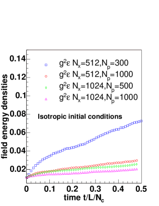
Fig. 1.: Time evolution of the average field energy density for isotropic particle momentum distributions on two different lattices (with the same physical size $L$) and for varying number of test particles. $N_{c}=2$ color simulations.

To check the numerical accuracy, we have first performed simulations for isotropic momentum distributions, varying the lattice spacing and the number of test-particles (Fig. 1). The field energy density is determined from the lattice field strength $\bm{E}_{L}\equiv ga^{2}\bm{E}$ as $g^{2}\epsilon=(1/2)\bm{E}_{L}^{2}/a^{4}$, plus the magnetic contribution. One observes that the time evolution stabilizes with increasing number of test-particles and decreasing lattice spacing. However, to reach sufficient accuracy our runs required several hundred to a thousand test-particles per lattice site, corresponding to $\approx 6$ hours run-time on a single-processor 2.4 GHz Opteron workstation per initial condition. It is therefore clear that a simple-minded extension of the point-particle algorithm to 3D-3V simulations is impossible. For multi-dimensional simulations, a generalization of current smearing from U(1) [8] to non-Abelian gauge groups is essential. Non-Abelian simulations which include fluctuations of the fields in the transverse plane would be very interesting because of indications that this leads to the development of a turbulent cascade which transfers energy from the soft unstable modes to stable UV field modes (near $k\sim 1/a$). This process, which is due to the self-interaction of the gauge field in the SU(2) theory, effectively tames the exponential growth of the fields [9].

3 Anisotropic initial distribution

In what follows, we consider anisotropic initial momentum distributions of the hard gluons,

$$f(\bm{p},\bm{x})\propto\exp(-\sqrt{p_{y}^{2}+p_{z}^{2}}/p_{\mathrm{hard}})\,\delta(p_{x})~{}.$$ (8)

This represents a quasi-thermal distribution in two dimensions, with “temperature” $=p_{\mathrm{hard}}$.

The initial field amplitudes are sampled from a Gaussian distribution with a width tuned to a given initial energy density. We solve the Yang-Mills equations in $A^{0}=0$ gauge and also set $\bm{A}=0$ at time $t=0$; the initial electric field is taken to be polarized in a random direction transverse to the $x$-axis. This initial condition is convenient because Gauss’s law $D_{i}E^{i}=\rho$ then implies local (color) charge neutrality at $t=0$, allowing for a straightforward initialization. Of course, magnetic and longitudinal electric field components quickly build up as time progresses.

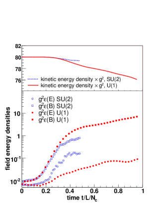
Fig. 2.: Time evolution of the kinetic (particle), and magnetic and electric field energy densities for $U(1)$ and $SU(2)$ gauge group, respectively.

We first show results for a relatively large separation of initial particle and field energy densities which should qualitatively resemble the conditions studied in [3, 9]. The results shown in Fig. 2 correspond to a lattice of physical size $L=40$ fm and $N_{x}=1024$ sites (the plots shown in ref. [4] correspond to the same $L$ but half the number of lattice sites). The hard scale was chosen as $p_{\mathrm{hard}}=10$ GeV (in lattice units, $p_{L,hard}=ap_{hard}$), and the particle density $g^{2}n=10$ fm^-3 (we define the density in lattice units as $n_{L}=g^{2}a^{3}n$). The above definitions of the lattice hamiltonian, fields and phase-space distribution function remove any explicit reference to the gauge coupling $g$ from the lattice theory.

For the Abelian theory we observe a rapid exponential growth of the magnetic field energy density, starting at about $t/L\approx 0.1$; we repeat that in order to avoid a “fake” growth of the fields during this initial transient time, one has to ensure that the number of test particles is sufficiently large. At a time $t/L\approx 0.4$ the magnetic field strength has grown by about one order of magnitude. The fields clearly affect the particles, which loose energy. In turn, at this time the exponential growth of the magnetic fields is slowed down. The electric field grows less rapidly and equipartitioning is not achieved within the depicted time interval.

The non-Abelian case features a rather similar evolution for short times ($t/L/N_{c}\approx 0.2$ for electric fields and $\approx 0.3$ for magnetic fields, respectively). We scaled time by $1/N_{c}$ because such a scaling is natural in the linear regime [3]. The growth of the magnetic field then saturates somewhat earlier than for the U(1) theory, and due to commutators, the electric field has more strength by the end of the simulation. Due to the somewhat earlier saturation of the instability, the colored particles loose less of their energy to the fields than was the case for electric charges. Nevertheless, at a purely qualitative level the $U(1)$ and $SU(2)$ simulations are not extremely different, which is due to the phenomenon of “Abelianization” in 1D-3V simulations [2, 3]. This does not occur in 3D.

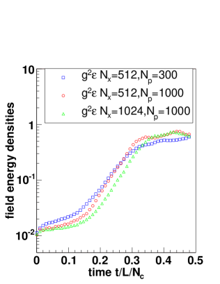
Fig. 3.: Time evolution of the field energy density on two different lattices (with the same physical size $L$); $N_{p}$ denotes the number of test particles per lattice site.

In Fig. 3 we compare results obtained on two different lattices with $N_{x}=512$ and $N_{x}=1024$ sites, respectively, for the same set of physical parameters. One observes that the growth rate of the instability, the saturation level and time are nearly the same. This confirms the underlying physical picture that the dynamics is dominated by the unstable soft field modes rather than UV-modes near the end of the Brioullin zone. If field modes with $k\sim 1/a$ would affect the dynamics then the continuum limit would not exist.

Our 1D-3V simulations thus clearly confirm the existence of instabilities in non-Abelian plasmas and the idea of “Abelianization”, namely that the field growth is perhaps damped by self-interactions but does not shut down until the fields have grown so much as to affect the motion of the particles. Nevertheless, the number of $e$-foldings by which the field energy density grows is much less spectacular in our simulations than for simulations within the “hard-loop” approximation [3]. This is due to the fact that our initial field amplitudes are already relatively large (non-linear regime). At a technical level, point-particle simulations are not very well suited to study the extreme weak-field regime, which would require a prohibitively large number of particles.

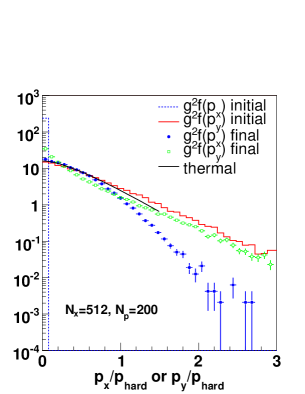
Fig. 4.: Initial and final particle distribution functions for the strong field case on a $N_{x}=512$ lattice.

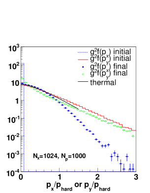
Fig. 5.: Same as Fig. 5 for a $N_{x}=1024$ lattice.

Once the fields have grown strong, they deflect the particles from their straight-line trajectories and finally lead to isotropization of their momentum distributions, shown explicitly in refs. [4]. This process represents the dominant contribution to the build-up of longitudinal pressure. Figs. 5,5 depict the evolution of the particle distribution function. This result was obtained with “strong-field” initial conditions: $p_{\mathrm{hard}}=1$ GeV and initial field energy density $\approx 10^{-1}$ GeV/fm${}^{3}/g^{2}$; the time scale is set by the lattice size, $L=10$ fm for this simulation. When the separation between hard and soft modes is not so large, strong instabilities can not develop as the system approaches isotropy very quickly [4].

In fact, propagation in strong random fields not only leads to isotropic but even to nearly exponential particle momentum distributions, as can be seen from Fig. 5. All particles with momenta up to $\sim p_{hard}$ appear to be more or less thermalized. Once again, we check the dependence on the lattice spacing by comparing results obtained on different lattices. We confirm numerically that the process does not appear to be dominated by the ultraviolet modes of the fields on the lattice.

Field fluctuations generate an effective collision term mediating soft exchanges. Defining

$$f(x,p,Q)=\langle f\rangle+\delta f,\quad A^{a}_{\mu}=\langle A^{a}_{\mu}\rangle+\delta A^{a}_{\mu},$$ (9)

where $\langle\ \rangle$ denotes the ensemble average, and $\langle\delta f\rangle=\langle\delta A^{a}_{\mu}\rangle=0$, one can obtain the Balescu-Lenard collision term from the fluctuation part, showing the correspondence between fluctuations and collisions in an Abelian plasma [10]. For the non-Abelian case, see refs. [11]. We also note that the mean entropy density is no longer conserved in the presence of fluctuations.

References

-
[1]
QGPTH05, Workshop on Quark-Gluon-Plasma Thermalization, August
10 – 12, 2005, TU Wien, Austria;
http://hep.itp.tuwien.ac.at/qgpth05
- [2] S. Mrowczynski, “Instabilities driven equilibration of the quark-gluon plasma,” arXiv:hep-ph/0511052, and references therein.
-
[3]
P. Romatschke and M. Strickland,
Phys. Rev. D 68, 036004 (2003);
Phys. Rev. D 70, 116006 (2004);
S. Mrowczynski, A. Rebhan and M. Strickland, Phys. Rev. D 70, 025004 (2004);
P. Arnold, J. Lenaghan and G. D. Moore, JHEP 0308, 002 (2003);
P. Arnold and J. Lenaghan, Phys. Rev. D 70, 114007 (2004);
P. Arnold, J. Lenaghan, G. D. Moore and L. G. Yaffe, Phys. Rev. Lett. 94, 072302 (2005);
A. Rebhan, P. Romatschke and M. Strickland, Phys. Rev. Lett. 94, 102303 (2005);
P. Romatschke and R. Venugopalan, arXiv:hep-ph/0510121. -
[4]
A. Dumitru and Y. Nara, Phys. Lett. B 621, 89 (2005);
Y. Nara, nucl-th/0509052. -
[5]
S. K. Wong, Nuovo Cim. A 65, 689 (1970);
U. W. Heinz, Nucl. Phys. A 418 (1984) 603C. -
[6]
P. F. Kelly, Q. Liu, C. Lucchesi and C. Manuel,
Phys. Rev. D 50, 4209 (1994);
J. P. Blaizot and E. Iancu, Phys. Rept. 359, 355 (2002). -
[7]
C. R. Hu and B. Müller,
Phys. Lett. B 409, 377 (1997);
G. D. Moore, C. R. Hu and B. Müller, Phys. Rev. D 58, 045001 (1998). - [8] J. Villasenor and O. Buneman, Comp. Phys. Comm. 69, 306 (1992).
-
[9]
P. Arnold, G. D. Moore and L. G. Yaffe,
Phys. Rev. D 72, 054003 (2005);
A. Rebhan, P. Romatschke and M. Strickland, JHEP 0509, 041 (2005);
P. Arnold and G. D. Moore, arXiv:hep-ph/0509206; arXiv:hep-ph/0509226. - [10] E. M. Lifshitz and L. P. Pitaevskii, Landau and Lifshitz Course of Theoretical Physics Vol. 10: “Physical Kinetics”; Pergamon Press, Oxford, 1981.
-
[11]
D. F. Litim and C. Manuel,
Phys. Rev. Lett. 82, 4981 (1999);
Nucl. Phys. B 562, 237 (1999);
D. Bödeker, Nucl. Phys. B 559 (1999) 502.