Electromagnetic radiative corrections in parity-violating electron-proton scattering

Abstract

QED radiative corrections have been calculated for leptonic and hadronic variables in parity-violating elastic ep scattering. For the first time, the calculation of the asymmetry in the elastic radiative tail is performed without the peaking-approximation assumption in hadronic variables configuration. A comparison with the PV-A4 data validates our approach. This method has been also used to evaluate the radiative corrections to the parity-violating asymmetry measured in the G0 experiment. The results obtained are here presented.

1 Introduction

Elastic scattering of longitudinally polarized electrons is subject to parity violation through the interference between $\gamma$ and $Z^{0}$ exchange. These experiments give access to the weak nucleon form factors (FF), which are the equivalent, in the weak sector, of the usual electromagnetic form factors $G_{E}$ and $G_{M}$. The weak nucleon form factors are related in turn to the strange form factors $G_{{}_{E}}^{{}^{{\scriptstyle s}}}$ and $G_{{}_{M}}^{{}^{{\scriptstyle s}}}$ , which are the contributions of strange currents to the form factors (see km88 and the following review articles ks00 ; mus94 ; bh01 ; bm01 ). According to QCD, this strangeness contribution arises from the presence of $s$$\bar{s}$ pairs in the nucleon sea. Many experiments have been performed recently or are still running at Bates (SAMPLE bps05 ; ito04 ; spa04 ), Mainz (PV-A4 maa04-1 ; maa04-2 ) and Jefferson Lab ($G^{0}$ arm05 and HAPPEX ani04 ).

Electromagnetic radiation produced from the emission of a real or virtual photon by the electron (incoming or outgoing) or by the target (before or after interaction), gives rises to a radiative tail which extends to very low energies (in theory, down to zero energy for the scattered electron). Since detectors have an experimental resolution and since cuts are used in the data analysis, the measured cross section and asymmetry have to be corrected in order to be compared to theoretical models. The first calculations applied to elastic ep scattering were done by Tsai tsa61 , followed by a series of review papers mt69 ; max69 ; tsa74 . This formalism has been later extended to scattering of polarized electrons mp00 . All these calculations were done for experiments in which the scattered electron is detected, which was the case of SAMPLE, PV-A4, HAPPEX or $G^{0}$ at backward angles back . The originality of the $G^{0}$ experiment at forward angles was the detection of recoil protons. In this case, some of the approximations commonly used when scattered electrons are detected, such as the peaking approximation, are no more valid. Thanks to its large mass, radiative emission from the proton is negligible but the proton kinematics is affected by the radiative emission from the electron (angle, energy, $Q^{2}$).

QED radiative corrections have been calculated for hadronic kinematic variables in $ep$ elastic scattering  afa01 and applied to recoil proton polarization. In this case, a method based on an electron structure-function representation, which is the analog of the Drell-Yann representation dy70 , was used. These calculations were applied to ep scattering experiments done at Jefferson Lab jon00 , aiming to determine the ratio of electric to magnetic proton form factors $G_{{}_{\!E}}^{{}^{p}}$/$G_{{}_{\!M}}^{{}^{p}}$at high momentum transfer as proposed by Akhiezer and Rekalo ar74 . The classical method for computing corrections is based on the separation of the momentum phase space into hard- and soft-photons contributions to avoid infrared divergences tsa61 . This introduces a cutoff parameter which makes this method not easily applicable to construct an event operator. Bardin and Shumeiko bs77 proposed a covariant cancellation method of infrared divergences which does not introduce additional parameters, however a cutoff has still to be introduced for generating real radiated photons.

In the present work we calculate the corrections in both the leptonic and hadronic variables using an original method which is free of infrared divergences. Its interest is that it is exact and it can be integrated easily into numerical simulation programs such as GEANT. We then apply it to $G^{0}$ forward angles using the G0-GEANT code g0geant . Another original feature of the present calculation is the inclusion of $Z^{0}$ exchange, in addition to $\gamma$ exchange, allowing to calculate the electroweak asymmetry of the radiative tail. We then calculate the corrected quantities of interest: integrated number of counts, time-of-flight (tof) spectra, $Q^{2}$ distributions. A full account of the present calculations is given in the thesis of Hayko Guler gul03 (in French).

In section 2 we develop the formalism and define the Lagrangians, in section 3 we describe our method for avoiding divergences, in section 4 we describe the $G^{0}$ apparatus and simulation method. The results are given in section 5 and we conclude in section 6.

2 Theoretical formalism for elastic scattering

The data analysis of parity-violating electron-nucleon scattering experiments involve the extraction of an asymmetry in the helicity-correlated cross section. The raw data are first converted into an experimentally measured asymmetry $(A_{exp})$. That means that the false asymmetry due to helicity-correlated fluctuations in intensity, energy, positions and angles of the electron beam have already been taken into account. We assume also that background subtraction has already been done.

The asymmetry is commonly defined as:

$$A=\frac{{(\frac{d\sigma}{d\Omega})}^{+}-{(\frac{d\sigma}{d\Omega})}^{-}}{{(\frac{d\sigma}{d\Omega})}^{+}+{(\frac{d\sigma}{d\Omega})}^{-}}$$ (1)

where ${(\frac{d\sigma}{d\Omega})}^{+}$ et ${(\frac{d\sigma}{d\Omega})}^{-}$ are the cross sections associated with incident electrons having helicity plus and minus respectively. The plus (minus) helicity corresponds to the spin of the electron being aligned and in the same direction as (opposite to) its momentum. Calculation of the cross section requires the knowledge of the amplitudes which are derived from the currents in the Feynman formalism.

The elastic scattering amplitude has two components corresponding to the electromagnetic part $\mathcal{M}_{\bf\gamma}$ and to the weak part $\mathcal{M}_{\bf Z}$

$$\hskip 17.07164pt\mathcal{M}\left(k^{\prime},p^{\prime},h_{e^{\prime}},h_{{}_{p^{\prime}}},k,p,h_{e},h_{{}_{p}}\right)$$

$$=\sum_{i=\gamma,Z}\mathcal{M}_{i}\left(k^{\prime},p^{\prime},h_{e^{\prime}},h_{{}_{p^{\prime}}},k,p,h_{e},h_{{}_{p}}\right)\hskip 28.45274pt$$ (2)

where $k$ and $k^{\,\prime}$ are the incident and scattered electron, $p$ and $p^{\,\prime}$ are the incident and recoil proton momentum respectively. $h_{e},h_{{}_{p}}$ and $h_{e^{\prime}},h_{{}_{p^{\prime}}}$ are the electron and proton helicity in the initial and final state.

$$\mathcal{M}_{\bf\gamma} = -ie^{2}~{}~{}\frac{1}{q^{2}}~{}{J^{{}^{P}}}_{\nu\hskip 2.84526ptem}\ {j^{\nu}}_{{}_{\scriptstyle\,em}}\hskip 19.91692pt$$ (3)

where ${j^{\nu}}_{{}_{\scriptstyle\,em}}$ is the Dirac leptonic electromagnetic current:

$${j^{\nu}}_{{}_{\scriptstyle\,em}} = \bar{u}(k^{\prime},h_{e^{\prime}})~{}\gamma^{\nu}~{}u(k,h_{e})$$ (4)

and ${J^{{}^{P}}}_{\nu\hskip 2.84526ptem}$ is the hadronic part of the electromagnetic current. The weak amplitude is given by:

$$\mathcal{M}_{\bf Z} = -i\frac{G}{2\sqrt{2}}~{}~{}\frac{1}{1-q^{2}/{\mbox{$M_{{}_{Z}}$}^{\!\!2}}}\hskip 73.97716pt$$ (5)

$$\bigg{\{}\hskip 8.53581pt\Big{(}{J^{{}^{P}}}_{\nu\hskip 2.84526ptnc}+{J^{{}^{P}}}_{\nu\hskip 2.84526ptnc5}\Big{)}j^{\nu}_{{}_{\bf weak}}\$$

$$\hskip 5.69054pt-\Big{(}{J^{{}^{P}}}_{nc}^{\nu}+{J^{{}^{P}}}_{nc5}^{\nu}\Big{)}\ \frac{q_{\nu}q_{\mu}}{\mbox{$M_{{}_{Z}}$}^{2}}\ j^{\mu}_{{}_{\bf weak}}\ \bigg{\}}$$

and the weak currents are obtained from:

$$j^{\mu}_{{}_{V}} =g_{V}^{e}\ \bar{u}(k^{\prime},h_{e^{\prime}})\ \gamma^{\mu}\ u(k,h_{e})$$ (6)

$$j^{\mu}_{{}_{A}} =g_{A}^{e}\ \bar{u}(k^{\prime},h_{e^{\prime}})\ \gamma^{\mu}\gamma^{5}\ u(k,h_{e})$$ (7)

$$j^{\mu}_{{}_{\bf weak}} =j^{\mu}_{{}_{V}}+j^{\mu}_{{}_{A}}$$ (8)

where $G$ is the Fermi constant, $g_{V}^{e}$ and $g_{A}^{e}$ are the weak vector and axial charges respectively. For electron scattering and at tree level they reduce to $g_{V}^{e}=\mbox{$-1+4\sin^{2}\theta_{{}_{W}}$}$ and $g_{A}^{e}=1$ respectively.

${J^{{}^{P}}}_{\nu\hskip 2.84526ptnc}$ and ${J^{{}^{P}}}_{\nu\hskip 2.84526ptnc5}$ are the hadronic weak currents. The hadronic structure is parametrized in terms of form factors:

$$J^{EM\mu}=<x^{\prime}|{\hat{J}}^{EM\mu}|x>$$ (9)

$$=\mbox{${\scriptstyle\overline{\cal U}}$}_{x^{\prime}}[\mbox{$F_{{}_{\!1}}^{{}^{x}}$}(Q^{2})\gamma^{\mu}+i\frac{\mbox{$F_{{}_{\!2}}^{{}^{x}}$}(Q^{2})}{2M}\sigma^{\mu\nu}q_{\nu}]\ \mbox{${\scriptstyle\cal U}$}_{x}$$ (10)

$$J^{NC\mu}=<x^{\prime}|{\hat{J}}^{NC\mu}|x>$$ (11)

$$=\mbox{${\scriptstyle\overline{\cal U}}$}_{x^{\prime}}[\mbox{$\widetilde{F}_{{}_{\!1}}^{{}^{x}}$}(Q^{2})\gamma^{\mu}+i\frac{\mbox{$\widetilde{F}_{{}_{\!2}}^{{}^{x}}$}(Q^{2})}{2M}\sigma^{\mu\nu}q_{\nu}]\ \mbox{${\scriptstyle\cal U}$}_{x}$$ (12)

$$J^{NC\mu 5}=<x^{\prime}|{\hat{J}}^{NC\mu 5}|x>$$ (13)

$$=\mbox{${\scriptstyle\overline{\cal U}}$}_{x^{\prime}}[\mbox{$\widetilde{G}_{{}_{\!A}}^{{}^{x}}$}(Q^{2})\gamma^{\mu}+i\frac{\mbox{$\widetilde{G}_{{}_{\!P}}^{{}^{x}}$}(Q^{2})}{M}q^{\mu}]\gamma^{5}\ \mbox{${\scriptstyle\cal U}$}_{x}$$ (14)

where $x=p,n$ represents a proton $p$ or a neutron $n$ and $\mbox{${\scriptstyle\cal U}$}_{x}$ and $\mbox{${\scriptstyle\overline{\cal U}}$}_{x^{\prime}}$ are the Dirac spinors for the nucleon in the entrance and exit channel respectively. $F_{{}_{\!1}}^{{}^{x}}$ and $F_{{}_{\!2}}^{{}^{x}}$ are the electromagnetic form factors, $\widetilde{F}_{{}_{\!1}}^{{}^{x}}$ and $\widetilde{F}_{{}_{\!2}}^{{}^{x}}$ are the neutral weak vector form factors and $\widetilde{G}_{{}_{\!A}}^{{}^{x}}$ and $\widetilde{G}_{{}_{\!P}}^{{}^{x}}$ are respectively the axial and pseudo-scalar form factors. The latter enters in the cross section and asymmetry through a $\mathcal{M}_{\bf Z}$ squared term which is totally negligible.

The observables are usually expressed in terms of the Sachs form factors $G_{{}_{\!E}}^{{}^{x}}$, $G_{{}_{\!M}}^{{}^{x}}$, $\widetilde{G}_{{}_{\!E}}^{{}^{x}}$ and $\widetilde{G}_{{}_{\!M}}^{{}^{x}}$ rather than the Fermi and Dirac form factors $F_{{}_{\!1}}^{{}^{x}}$, $F_{{}_{\!2}}^{{}^{x}}$, $\widetilde{F}_{{}_{\!1}}^{{}^{x}}$, $\widetilde{F}_{{}_{\!2}}^{{}^{x}}$ :

$$\mbox{$G_{{}_{\!E}}^{{}^{x}}$}(Q^{2})=\mbox{$F_{{}_{\!1}}^{{}^{x}}$}(Q^{2})-\tau\mbox{$F_{{}_{\!2}}^{{}^{x}}$}(Q^{2})$$ (15)

$$\mbox{$G_{{}_{\!M}}^{{}^{x}}$}(Q^{2})=\mbox{$F_{{}_{\!1}}^{{}^{x}}$}(Q^{2})+\mbox{$F_{{}_{\!2}}^{{}^{x}}$}(Q^{2})$$ (17)

$$\mbox{$\widetilde{G}_{{}_{\!E}}^{{}^{x}}$}(Q^{2})=\mbox{$\widetilde{F}_{{}_{\!1}}^{{}^{x}}$}(Q^{2})-\tau\mbox{$\widetilde{F}_{{}_{\!2}}^{{}^{x}}$}(Q^{2})$$

$$\mbox{$\widetilde{G}_{{}_{\!M}}^{{}^{x}}$}(Q^{2})=\mbox{$\widetilde{F}_{{}_{\!1}}^{{}^{x}}$}(Q^{2})+\mbox{$\widetilde{F}_{{}_{\!2}}^{{}^{x}}$}(Q^{2})$$ (18)

where $\tau$ is a kinematic factor defined as $\tau=\frac{{Q}^{2}}{4{{M}_{p}}^{2}}$ and ${M}_{p}$ is the proton mass.

The helicity-correlated cross section is given by:

$$\frac{d^{2}\sigma_{{}_{\scriptstyle h_{e}}}}{d\Omega_{e^{\prime}}}=\frac{1}{16(2\pi)^{2}}\;\frac{|\vec{k}^{\,\prime}|^{2}}{M\,|\vec{k}|}\hskip 113.81102pt$$

$$\hskip 42.67912pt\frac{1}{2}\ \frac{\sum^{\prime}|{\mathcal{M}}|^{2}}{\Big{|}E_{p^{\prime}}|\vec{k}^{\,\prime}|+E_{e^{\prime}}(|\vec{k}^{\,\prime}|-|\vec{k}|\cos(\theta_{e^{\prime}}))\Big{|}}$$ (19)

where the summation $\sum^{\prime}$ is performed over all the spin variables except the incident electron helicity. The asymmetry can then be calculated from Eq. (1):

$${A}_{{}_{LR}}(\vec{e}N)=-\frac{{G}_{F}{Q}^{2}}{4\pi\alpha\sqrt{2}}\frac{1}{\varepsilon{(\mbox{$G_{{}_{\!E}}^{{}^{x}}$})}^{2}+\tau{(\mbox{$G_{{}_{\!M}}^{{}^{x}}$})}^{2}}$$ (20)

$$\bigg{\{}\varepsilon\,\mbox{$G_{{}_{\!E}}^{{}^{x}}$}\,\mbox{$\widetilde{G}_{{}_{\!E}}^{{}^{x}}$}+\tau\,\mbox{$G_{{}_{\!M}}^{{}^{x}}$}\,\mbox{$\widetilde{G}_{{}_{\!M}}^{{}^{x}}$}-(1-4\,{\sin}^{2}{\theta}_{{}_{W}})\,\varepsilon^{\prime}\,\mbox{$G_{{}_{\!M}}^{{}^{x}}$}\,\mbox{$\widetilde{G}_{{}_{\!A}}^{{}^{x}}$}\bigg{\}}$$ (21)

in which the $Q^{2}$ dependence has been omitted for clarity of notation. $\epsilon$, $\epsilon^{\prime}$ are kinematic factors given by:

$$\epsilon=\frac{1}{1+2(1+\tau){\tan}^{2}\frac{\theta_{e^{\prime}}}{2}}$$ (22)

$$\hskip 28.45274pt\epsilon^{\prime}=\sqrt{\tau(1+\tau)(1-{\epsilon}^{2})}$$ (23)

$\theta_{e}^{\prime}$ is the electron scattering angle and ${\theta}_{W}$ is the Weinberg angle.

The ultimate purpose of these experiments being to determine the strange content of the nucleon, one must isolate the contribution of the $s$-quark in the nucleon form factors. In order to do that, we decompose the electromagnetic, neutral and axial currents according to the different flavor contributions $f=u,d,s$:

$$<x^{\prime}|{\bar{u}}_{f}{\gamma}_{\mu}{u}_{f}|x>\equiv$$ (24)

$$\mbox{${\scriptstyle\overline{\cal U}}$}_{x^{\prime}}\Big{(}\mbox{$F_{{}_{\!1}}^{{}^{f,x}}$}(Q^{2})\gamma_{\mu}+i\frac{\mbox{$F_{{}_{\!2}}^{{}^{f,x}}$}(Q^{2})}{2M}\sigma_{\mu\nu}q^{\nu}\Big{)}\ \mbox{${\scriptstyle\cal U}$}_{x}$$ (26)

$$<x^{\prime}|{\bar{u}}_{f}{\gamma}_{\mu}{\gamma}_{5}{u}_{f}|x>\equiv$$

$$\mbox{${\scriptstyle\overline{\cal U}}$}_{x^{\prime}}\Big{(}\mbox{$\widetilde{G}_{{}_{A}}^{{}^{f,x}}$}(Q^{2})\gamma_{\mu}+i\frac{\mbox{$\widetilde{G}_{{}_{P}}^{{}^{f,x}}$}(Q^{2})}{M}q_{\mu}\Big{)}\,\gamma_{5}\,\mbox{${\scriptstyle\cal U}$}_{x}$$ (27)

where $u_{f}$ and $\bar{u}_{f}$ are the quarks fields. The pseudo-scalar form factors $\widetilde{G}_{{}_{P}}^{{}^{f,x}}$ being ignored, there are 18 form factors to be evaluated: 9 for the proton and 9 for the neutron. In order to reduce that number we use charge symmetry, assuming that the $p$ and the $n$ are members of a perfect isospin doublet. Omitting the $Q^{2}$-dependence:

$$\mbox{$F_{{}_{\!1}}^{{}^{u}}$}\equiv\mbox{$F_{{}_{\!1}}^{{}^{u,p}}$}=\mbox{$F_{{}_{\!1}}^{{}^{d,n}}$}\hskip 28.45274pt\mbox{$F_{{}_{\!2}}^{{}^{u}}$}\equiv\mbox{$F_{{}_{\!2}}^{{}^{u,p}}$}=\mbox{$F_{{}_{\!2}}^{{}^{d,n}}$}$$ (28)

$$\mbox{$F_{{}_{\!1}}^{{}^{d}}$}\equiv\mbox{$F_{{}_{\!1}}^{{}^{d,p}}$}=\mbox{$F_{{}_{\!1}}^{{}^{u,n}}$}\hskip 28.45274pt\mbox{$F_{{}_{\!2}}^{{}^{d}}$}\equiv\mbox{$F_{{}_{\!2}}^{{}^{d,p}}$}=\mbox{$F_{{}_{\!2}}^{{}^{u,n}}$}$$ (29)

$$\mbox{$F_{{}_{\!1}}^{{}^{s}}$}\equiv\mbox{$F_{{}_{\!1}}^{{}^{s,p}}$}=\mbox{$F_{{}_{\!1}}^{{}^{s,n}}$}\hskip 28.45274pt\mbox{$F_{{}_{\!2}}^{{}^{s}}$}\equiv\mbox{$F_{{}_{\!2}}^{{}^{s,p}}$}=\mbox{$F_{{}_{\!2}}^{{}^{s,n}}$}$$ (30)

$$\mbox{$G_{{}_{A}}^{{}^{u}}$}\equiv\mbox{$\widetilde{G}_{{}_{A}}^{{}^{u,p}}$}=\mbox{$\widetilde{G}_{{}_{A}}^{{}^{d,n}}$}$$ (31)

$$\hskip 14.22636pt\mbox{$G_{{}_{A}}^{{}^{d}}$}\equiv\mbox{$\widetilde{G}_{{}_{A}}^{{}^{d,p}}$}=\mbox{$\widetilde{G}_{{}_{A}}^{{}^{u,n}}$}$$ (32)

$$\hskip 14.22636pt\mbox{$G_{{}_{A}}^{{}^{s}}$}\equiv\mbox{$\widetilde{G}_{{}_{A}}^{{}^{s,p}}$}=\mbox{$\widetilde{G}_{{}_{A}}^{{}^{s,n}}$}$$ (33)

After some algebra arv05 , the asymmetry can be finally expressed in terms of the electromagnetic, axial and strange nucleon form factors:

$${A}_{{}_{LR}}(\vec{e}p)=-\frac{{G}_{F}{Q}^{2}}{4\pi\alpha\sqrt{2}}\bigg{\{}\hskip 5.69054pt(1-4{\sin}^{2}{\theta}_{{}_{W}})(1+\mbox{$R_{{}_{V}}^{{}^{p}}$})$$

$$\hskip 34.1433pt-(1+\mbox{$R_{{}_{V}}^{{}^{n}}$})\frac{\varepsilon\mbox{$G_{{}_{\!E}}^{{}^{p}}$}\mbox{$G_{{}_{\!E}}^{{}^{n}}$}+\tau\mbox{$G_{{}_{\!M}}^{{}^{p}}$}\mbox{$G_{{}_{\!M}}^{{}^{n}}$}}{\varepsilon{(\mbox{$G_{{}_{\!E}}^{{}^{p}}$})}^{2}+\tau{(\mbox{$G_{{}_{\!M}}^{{}^{p}}$})}^{2}}\bigg{\}}$$

$$\hskip 34.1433pt+\frac{{G}_{F}{Q}^{2}}{4\pi\alpha\sqrt{2}}\hskip 5.69054pt(1+\mbox{$R_{{}_{V}}^{{}^{(0)}}$})\frac{\varepsilon\mbox{$G_{{}_{\!E}}^{{}^{p}}$}}{\varepsilon{(\mbox{$G_{{}_{\!E}}^{{}^{p}}$})}^{2}+\tau{(\mbox{$G_{{}_{\!M}}^{{}^{p}}$})}^{2}}\,\mbox{$G_{{}_{E}}^{{}^{{\scriptstyle s}}}$ }$$

$$\hskip 34.1433pt+\frac{{G}_{F}{Q}^{2}}{4\pi\alpha\sqrt{2}}\hskip 5.69054pt(1+\mbox{$R_{{}_{V}}^{{}^{(0)}}$})\frac{\tau\mbox{$G_{{}_{\!M}}^{{}^{p}}$}}{\varepsilon{(\mbox{$G_{{}_{\!E}}^{{}^{p}}$})}^{2}+\tau{(\mbox{$G_{{}_{\!M}}^{{}^{p}}$})}^{2}}\,\mbox{$G_{{}_{M}}^{{}^{{\scriptstyle s}}}$ }$$

$$\hskip 34.1433pt+\frac{{G}_{F}{Q}^{2}}{4\pi\alpha\sqrt{2}}\,\,\,\frac{(1-4{\sin}^{2}{\theta}_{{}_{W}})\,\varepsilon^{\prime}\mbox{$G_{{}_{\!M}}^{{}^{p}}$}}{\varepsilon{(\mbox{$G_{{}_{\!E}}^{{}^{p}}$})}^{2}+\tau{(\mbox{$G_{{}_{\!M}}^{{}^{p}}$})}^{2}}\,\,\mbox{$\widetilde{G}_{{}_{\!A}}^{{}^{p}}$}$$ (34)

The coefficients $R_{{}_{V}}^{{}^{p}}$, $R_{{}_{V}}^{{}^{n}}$and $R_{{}_{V}}^{{}^{(0)}}$are electroweak radiative corrections parameters which can be calculated within the Standard Model  pdg04 .

When recoil protons are detected instead of scattered electrons, the helicity-correlated cross section becomes:

$$\frac{d^{2}\sigma_{{}_{\scriptstyle h_{e}}}}{d\Omega_{p^{\prime}}}=\frac{1}{16(2\pi)^{2}}\;\frac{|\vec{p}^{\,\prime}|^{2}}{M\,|\vec{k}|}\hskip 113.81102pt$$

$$\hskip 42.67912pt\frac{1}{2}\ \frac{\sum^{\prime}|{\mathcal{M}}|^{2}}{\Big{|}E_{e^{\prime}}|\vec{p}^{\,\prime}|+E_{p^{\prime}}(|\vec{p}^{\,\prime}|-|\vec{k}|\cos(\theta_{p^{\prime}}))\Big{|}}$$ (35)

The asymmetry calculation follows the same steps as for scattered electron detection.

3 QED radiative corrections

3.1 Parity-violating experiment representation in leptonic variables

The aim of the procedure is to get a differential cross section $d^{3}\sigma/d\Omega_{e^{\prime}}dE_{e^{\prime}}$ without any singularity in the full electron spectrum. We divide the scattered electron energy interval into two regions. The first one, $E_{e^{\prime}\,min}\leq E_{e^{\prime}}\leq E_{e^{\prime}\,cut}$ where $E_{e^{\prime}\,cut}\equiv E_{e^{\prime}\,elas}-\Delta E_{e^{\prime}}$ corresponds to “hard photons” with a minimum energy $E_{e^{\prime}\,min}$ which may be of the order of few MeV. The second one is defined by $E_{e^{\prime}\,cut}\leq E_{e^{\prime}}\leq E_{e^{\prime}\,elas}$ which corresponds to the “soft photon” region. The maximum energy of the outgoing electron corresponds to the elastic peak and is denoted by $E_{e^{\prime}\,elas}$. The first requirement is that the integral

$$\int^{E_{e^{\prime}\,elas}}_{E_{e^{\prime}\,min}} \frac{d^{3}\sigma}{d\Omega_{e^{\prime}}dE_{e^{\prime}}}\,dE_{e^{\prime}}=\int^{E_{e^{\prime}\,cut}}_{E_{e^{\prime}\,min}}\frac{d^{3}\sigma}{d\Omega_{e^{\prime}}dE_{e^{\prime}}}\,dE_{e^{\prime}}$$ (36)

$$\hskip 28.45274pt+\int^{E_{e^{\prime}\,elas}}_{E_{e^{\prime}\,cut}}\frac{d^{3}\sigma}{d\Omega_{e^{\prime}}dE_{e^{\prime}}}\,dE_{e^{\prime}}$$

should be as much as possible independent of the cutoff energy $\Delta E_{e^{\prime}}$.

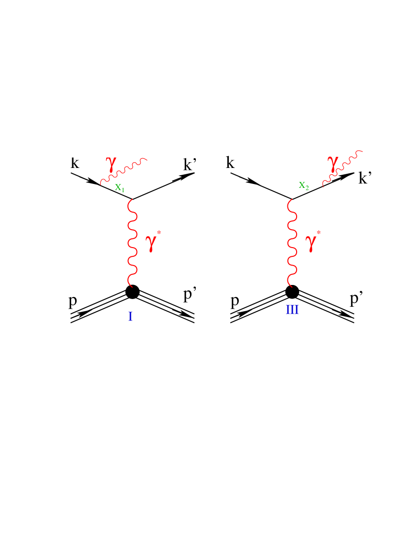
Figure 1: Real-photon emission in virtual-photon exchange

The three-dimensional differential cross section which appears in the first term in the right hand side of (36) is obtained from the five-dimensional differential cross section:

$$\frac{d^{3}\sigma}{d\Omega_{e^{\prime}}dE_{e^{\prime}}}=\int\frac{d^{5}\sigma}{d\Omega_{e^{\prime}}dE_{e^{\prime}}d\Omega_{\gamma}}\ d\Omega_{\gamma}$$ (37)

corresponding to the bremsstrahlung process $e+p\longrightarrow e+p+\gamma$. The two Feynman diagrams describing this process are displayed in Fig. 1. The integral defined in (37) may be calculated in the peaking approximation when the scattering angle of the detected electron is not too small, which is the case for most experiments. In particular, this approximation is very good for the PV-A4 experiment at forward angle ($30^{\circ}\leq\theta\leq 40^{\circ}$) and for the PV-A4 and $G^{0}$ experiments at backward angles. The final result is found to be mt69 ; orv :

$$\frac{d^{3}\sigma}{d\Omega_{e^{\prime}}dE_{e^{\prime}}}\approx\Big{[}\frac{d^{3}\sigma}{d\Omega_{e^{\prime}}dE_{e^{\prime}}}\Big{]}_{peaking}= \mathcal{K}_{s}\frac{d^{2}\sigma_{{}_{0}}(E_{e\,s},Q^{2}_{s})}{d\Omega_{e^{\prime}}}$$ (38)

$$+\mathcal{K}_{p}\frac{d^{2}\sigma_{{}_{0}}(E_{e},Q^{2}_{p})}{d\Omega_{e^{\prime}}}$$

where the index $0$ stands for the Born elastic differential cross section. The term with the $s$ (respectively $p$) index represents the contribution of the left (right) Feynman diagram of Fig. 1. The coefficients $\mathcal{K}_{s}$ and $\mathcal{K}_{p}$ are kinematic factors.

The second term in the right hand side of (36) is usually expressed as

$$\int^{E_{e^{\prime}\,elas}}_{E_{e^{\prime}\,cut}}\frac{d^{3}\sigma}{d\Omega_{e^{\prime}}dE_{e^{\prime}}}\,dE_{e^{\prime}}=\!\Big{(}1+\delta(\Delta E_{e^{\prime}})\Big{)}\ \frac{d^{2}\sigma_{{}_{0}}(E_{e},Q^{2})}{d\Omega_{e^{\prime}}}$$

where the theoretical expression of $\delta(\Delta E_{e^{\prime}})$ is given in  mt69 ; orv . The numerical calculation of the right hand side of Eq. (36) is shown in Fig. 2 for the PV-A4 parity-violating experiment. The minimum value of $\Delta E_{e^{\prime}}$ in this kinematics is about 2 MeV.

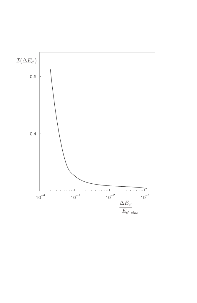
Figure 2: Dependence of the right hand side of Eq. (36) with $\Delta E_{e^{\prime}}$ in A4 experiment: $E_{e}$=0.855 GeV, $\theta_{e^{\prime}}$=35^∘

An analytic expression for the three-dimensional differential cross section in the energy range $E_{e^{\prime}\,cut}\leq E_{e^{\prime}}\leq E_{e^{\prime}\,elas}$ can be defined as:

$$\Big{(}\frac{d^{3}\sigma}{d\Omega_{e^{\prime}}dE_{e^{\prime}}}\Bigr{)}_{anal}=a_{{}_{0}}(\theta_{e^{\prime}})\,+\,a_{{}_{1}}(\theta_{e^{\prime}})\,E_{e^{\prime}}\,+\,a_{{}_{2}}(\theta_{e^{\prime}})\,E^{2}_{e^{\prime}}$$

The three parameters $a_{{}_{0}}$, $a_{{}_{1}}$ and $a_{{}_{2}}$ are fixed using the three conditions:

$$i) at\ E_{e^{\prime}}=E_{e^{\prime}\,cut}:$$ (43)

$$\Big{[}\frac{d^{3}\sigma}{d\Omega_{e^{\prime}}dE_{e^{\prime}}}\Big{]}_{peaking}=\Big{(}\frac{d^{3}\sigma}{d\Omega_{e^{\prime}}dE_{e^{\prime}}}\Bigr{)}_{anal}\hskip 28.45274pt$$

$$ii) at\ E_{e^{\prime}}=E_{e^{\prime}\,cut}:$$

$$\frac{\partial}{\partial E_{e^{\prime}}}\Big{[}\frac{d^{3}\sigma}{d\Omega_{e^{\prime}}dE_{e^{\prime}}}\Big{]}_{peaking}=\frac{\partial}{\partial E_{e^{\prime}}}\Big{(}\frac{d^{3}\sigma}{d\Omega_{e^{\prime}}dE_{e^{\prime}}}\Bigr{)}_{anal}$$

$$iii) \int^{E_{e^{\prime}\,elas}}_{E_{e^{\prime}\,cut}}\Big{(}\frac{d^{3}\sigma}{d\Omega_{e^{\prime}}dE_{e^{\prime}}}\Bigr{)}_{anal}\ dE_{e^{\prime}}=\Big{(}1+\delta(\Delta E_{e^{\prime}})\Big{)}$$

$$\hskip 113.81102pt\times\frac{d^{2}\sigma_{{}_{0}}(E_{e},Q^{2})}{d\Omega_{e^{\prime}}}$$

Full simulations performed with the Monte-Carlo method and the experimental setup in the angular range between $40^{\circ}\leq\theta^{\circ}\leq 30$ at $E_{e}=$ 0.855 GeV collin ; capozza have shown that the final spectrum is, within the experimental resolution, independent of the cutoff parameter $\Delta E_{e^{\prime}}$ when its value is increased by a factor 2 to 4. The good agreement between the model and the PV-A4 experiment can be seen in Fig. 3.

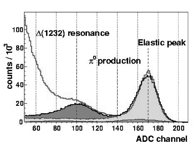
Figure 3: Comparison of the experimental (red solid line) and simulated spectra (filled grey areas) for the PV-A4 experiment capozza . The light-grey area corresponds to the simulated elastic ep scattering plus radiative corrections.

The simulated parity-violating asymmetry is then defined as:

$$A=\left\{\begin{array}[]{cc}A_{elas}&\hskip 2.84526ptE_{e^{\prime}\,cut}\leq E_{e^{\prime}}\leq E_{e^{\prime}\,elas}\\[5.69054pt] \frac{\displaystyle\mathcal{K}_{s}\sigma_{s}A_{s}+\mathcal{K}_{p}\sigma_{p}A_{p}}{\displaystyle\mathcal{K}_{s}\sigma_{s}+\mathcal{K}_{p}\sigma_{p}}&\ E_{e^{\prime}\,min}\leq E_{e^{\prime}}\leq E_{e^{\prime}\,cut}\end{array}\right.$$ (46)

where $\sigma_{i}\equiv d^{2}\sigma_{{}_{0}}(E_{e,s},Q^{2}_{i})/d\Omega_{e^{\prime}}$ , $i=s,p$. The asymmetries $A_{s}$ and $A_{p}$ are the Born asymmetries calculated for the kinematics of the $s$ and $p$ channels through the relations given in the previous section.

3.2 Parity-violating experiment in proton variables

We describe here the method developed to take into account the internal radiative corrections when the proton, instead of the electron, is detected. Again, we will obtain for the proton spectrum a differential cross section $d^{3}\sigma/d\Omega_{p^{\prime}}dE_{p^{\prime}}$ without any singularity. The extension of the method derived for the electrons will give also the parity-violating asymmetry in the proton channel. As in the electron case, we define $E_{p^{\prime}\,cut}\equiv E_{p^{\prime}\,elas}-\Delta E_{p^{\prime}}$ and we require the integral $\mathcal{\bf I}(\Delta E_{p^{\prime}})$

$$\int^{E_{p^{\prime}\,elas}}_{E_{p^{\prime}\,min}}\frac{d^{3}\sigma}{d\Omega_{p^{\prime}}dE_{p^{\prime}}}\,dE_{p^{\prime}}=\int^{E_{p^{\prime}\,cut}}_{E_{p^{\prime}\,min}}\frac{d^{3}\sigma}{d\Omega_{p^{\prime}}dE_{p^{\prime}}}\,dE_{p^{\prime}}$$

$$\hskip 28.45274pt+\int^{E_{p^{\prime}\,elas}}_{E_{p^{\prime}\,cut}}\frac{d^{3}\sigma}{d\Omega_{p^{\prime}}dE_{p^{\prime}}}\,dE_{p^{\prime}}$$ (47)

to be as much as possible independent of the energy cutoff $\Delta E_{p^{\prime}}$. We have to modify the method of the previous section for two reasons. First, as we detect the proton, the differential cross section is now given by

$$\frac{d^{3}\sigma}{d\Omega_{p^{\prime}}dE_{p^{\prime}}}=\int\frac{d^{5}\sigma}{d\Omega_{p^{\prime}}dE_{p^{\prime}}d\Omega_{\gamma}}\ d\Omega_{\gamma}$$ (48)

Very forward angles of the outgoing electrons are allowed when the integration over all the directions of the photon is performed, so the cross section has to be calculated at the amplitude level to be sure that gauge invariance is respected. Secondly, as we are interested to correct the experimental asymmetry from the internal radiative contribution, we need to introduce two more Feynman diagrams in the calculation, as shown in Fig. 4.

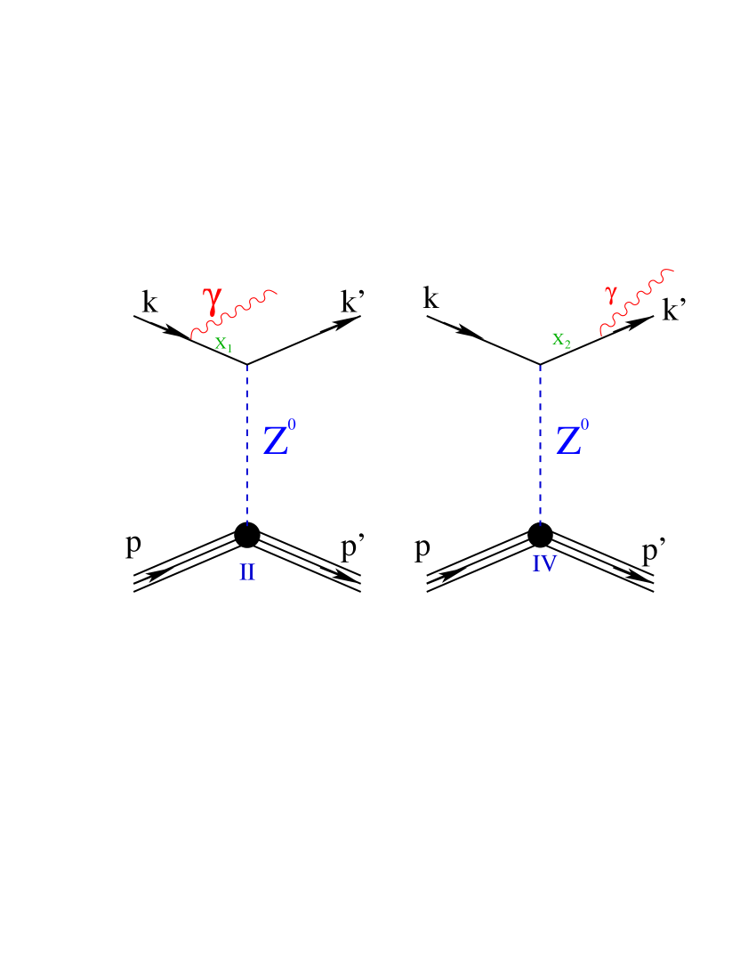
Figure 4: Real-photon emission in virtual-$Z^{0}$ exchange.

The amplitude of the reaction $e+p\longrightarrow e+p+\gamma$ is written as

$$\hskip 17.07164pt\mathcal{M}\left(k^{\prime},p^{\prime},h_{e^{\prime}},h_{{}_{p^{\prime}}},p_{\gamma},h_{\gamma},k,p,h_{e},h_{{}_{p}}\right)$$

$$=\sum_{i=\bf I,\cdots IV}\mathcal{M}_{i}\left(k^{\prime},p^{\prime},h_{e^{\prime}},h_{{}_{p^{\prime}}},p_{\gamma},h_{\gamma},k,p,h_{e},h_{{}_{p}}\right)\hskip 28.45274pt$$ (49)

The four-vectors of the exchanged photon and $Z^{0}$ propagators are expressed in terms of the kinematic variables:

$$\hskip 17.07164ptq=k-k^{\prime}-p_{\gamma}=p^{\prime}-p$$ (50)

$$x_{{}_{\scriptstyle 1}}=k-p_{\gamma}\hskip 28.45274ptx_{{}_{\scriptstyle 2}}=k^{\prime}+p_{\gamma}=k+p-p^{\prime}\hskip 14.22636pt$$ (51)

The amplitudes $\bf I$ and $\bf III$ due to the exchanged photon with the propagator $-ig_{\nu\nu^{\prime}}/q^{2}$ have one term:

$$\mathcal{M}_{\bf I} = ie^{3}~{}\frac{1}{x^{{}^{\scriptstyle 2}}_{{}_{\scriptstyle 1}}-m_{e}^{2}}~{}\frac{1}{q^{2}}~{}{J^{{}^{P}}}_{\nu\hskip 2.84526ptem}\ T^{\nu\mu}_{{}_{\bf I}\,em}~{}{\varepsilon_{\mu}}^{{}^{\star}}(p_{\gamma},h_{\gamma})\hskip 19.91692pt$$ (52)

$$T^{\nu\mu}_{{}_{\bf I}\,em} = \bar{u}(k^{\prime},h_{e^{\prime}})~{}\gamma^{\nu}~{}(\mbox{${\mbox{$x_{{}_{1}}$}}/$}+m_{e})\gamma^{\mu}~{}u(k,h_{e})$$ (53)

$$\mathcal{M}_{\bf III} = ie^{3}~{}\frac{1}{x^{{}^{\scriptstyle 2}}_{{}_{\scriptstyle 2}}-m_{e}^{2}}~{}\frac{1}{q^{2}}~{}{J^{{}^{P}}}_{\nu\hskip 2.84526ptem}\ T^{\mu\nu}_{{}_{\bf III}\,em}~{}{\varepsilon_{\mu}}^{{}^{\star}}(p_{\gamma},h_{\gamma})\hskip 17.07164pt$$ (54)

$$T^{\mu\nu}_{{}_{\bf III}\,em} = \bar{u}(k^{\prime},h_{e^{\prime}})~{}\gamma^{\mu}~{}(\mbox{${\mbox{$x_{{}_{2}}$}}/$}+m_{e})\gamma^{\nu}~{}u(k,h_{e})$$ (55)

while the amplitudes $\bf II$ and $\bf IV$ due to the exchange of the $Z^{0}$ with the propagator $i(-g_{\nu\nu^{\prime}}+q_{\nu}q_{\nu^{\prime}}/\mbox{$M_{{}_{Z}}$}^{2})/(q^{2}-\mbox{$M_{{}_{Z}}$}^{2})$ have each two different contributions:

$$\mathcal{M}_{\bf II} = ie~{}\frac{G}{2\sqrt{2}}~{}\frac{1}{x^{{}^{\scriptstyle 2}}_{{}_{\scriptstyle 1}}-m_{e}^{2}}~{}\frac{1}{1-q^{2}/{\mbox{$M_{{}_{Z}}$}^{\!\!2}}}\hskip 73.97716pt$$ (56)

$$\bigg{\{}\hskip 8.53581pt\Big{(}{J^{{}^{P}}}_{\nu\hskip 2.84526ptnc}+{J^{{}^{P}}}_{\nu\hskip 2.84526ptnc5}\Big{)}\hskip 2.84526ptT^{\nu\mu}_{{}_{\bf II}}\ {\varepsilon_{\mu}}^{{}^{\star}}(p_{\gamma},h_{\gamma})$$

$$\hskip 5.69054pt-\Big{(}{J^{{}^{P}}}_{nc}^{\nu^{\prime}}+{J^{{}^{P}}}_{nc5}^{\nu^{\prime}}\Big{)}\ \frac{q_{\nu}q_{\nu^{\prime}}}{\mbox{$M_{{}_{Z}}$}^{2}}\ T^{\nu\mu}_{{}_{\bf II}}\ {\varepsilon_{\mu}}^{{}^{\star}}(p_{\gamma},h_{\gamma})\bigg{\}}$$

$$T^{\nu\mu}_{{}_{{{\bf II}}\,V}} =g_{V}^{e}\ \bar{u}(k^{\prime},h_{e^{\prime}})\ \gamma^{\nu}(\mbox{${\mbox{$x_{{}_{1}}$}}/$}+m_{e})\gamma^{\mu}\ u(k,h_{e})$$ (57)

$$T^{\nu\mu}_{{}_{{\bf II}\,A}} =g_{A}^{e}\ \bar{u}(k^{\prime},h_{e^{\prime}})\ \gamma^{\nu}\gamma^{5}(\mbox{${\mbox{$x_{{}_{1}}$}}/$}+m_{e})\gamma^{\mu}\ u(k,h_{e})$$ (58)

$$T^{\nu\mu}_{{}_{\bf II}} =T^{\nu\mu}_{{}_{{\bf IV}\,V}}+T^{\nu\mu}_{{}_{{\bf IV}\,A}},$$ (59)

$$\mathcal{M}_{\bf IV} = ie~{}\frac{G}{2\sqrt{2}}~{}\frac{1}{x^{{}^{\scriptstyle 2}}_{{}_{\scriptstyle 2}}-m_{e}^{2}}~{}\frac{1}{1-q^{2}/{\mbox{$M_{{}_{Z}}$}^{\!\!2}}}\hskip 73.97716pt$$ (60)

$$\bigg{\{}\hskip 8.53581pt\Big{(}{J^{{}^{P}}}_{\nu\hskip 2.84526ptnc}+{J^{{}^{P}}}_{\nu\hskip 2.84526ptnc5}\Big{)}\hskip 2.84526ptT^{\mu\nu}_{{}_{\bf IV}}\ {\varepsilon_{\mu}}^{{}^{\star}}(p_{\gamma},h_{\gamma})$$

$$\hskip 5.69054pt-\Big{(}{J^{{}^{P}}}_{nc}^{\nu^{\prime}}+{J^{{}^{P}}}_{nc5}^{\nu^{\prime}}\Big{)}\ \frac{q_{\nu}q_{\nu^{\prime}}}{\mbox{$M_{{}_{Z}}$}^{2}}\ T^{\mu\nu}_{{}_{\bf IV}}\ {\varepsilon_{\mu}}^{{}^{*}}(p_{\gamma},h_{\gamma})\bigg{\}}$$

$$T^{\mu\nu}_{{}_{{\bf IV}\,V}} =g_{V}^{e}\ \bar{u}(k^{\prime},h_{e^{\prime}})\ \gamma^{\mu}(\mbox{${\mbox{$x_{{}_{2}}$}}/$}+m_{e})\gamma^{\nu}\ u(k,h_{e})$$ (61)

$$T^{\mu\nu}_{{}_{{\bf IV}\,A}} =g_{A}^{e}\ \bar{u}(k^{\prime},h_{e^{\prime}})\ \gamma^{\mu}(\mbox{${\mbox{$x_{{}_{2}}$}}/$}+m_{e})\gamma^{\nu}\gamma^{5}\ u(k,h_{e})$$ (62)

$$T^{\mu\nu}_{{}_{\bf IV}} =T^{\mu\nu}_{{}_{{\bf VI}\,V}}+T^{\mu\nu}_{{}_{{\bf VI}\,A}}$$ (63)

In the energy range where the parity-violating experiments are performed ($0.1\leq Q^{2}\leq 1$$(GeV/c)^{2}$ , terms proportional to $1/{\mbox{$M_{{}_{Z}}$}^{2}}$ are neglected, therefore:

$$\mathcal{M}_{\bf II} \approx ie~{}\frac{G}{2\sqrt{2}}~{}\frac{1}{x^{{}^{\scriptstyle 2}}_{{}_{\scriptstyle 1}}-m_{e}^{2}}\hskip 71.13188pt$$

$$\bigg{\{}\Big{(}{J^{{}^{P}}}_{\nu\hskip 2.84526ptnc}+{J^{{}^{P}}}_{\nu\hskip 2.84526ptnc5}\Big{)}\Big{(}T^{\nu\mu}_{{}_{{\bf II}\,V}}+T^{\nu\mu}_{{}_{{\bf IV}\,A}}\Big{)}\ {\varepsilon_{\mu}}^{{}^{\star}}(p_{\gamma},h_{\gamma})\bigg{\}}$$

and

$$\mathcal{M}_{\bf IV} \approx ie~{}\frac{G}{2\sqrt{2}}~{}\frac{1}{x^{{}^{\scriptstyle 2}}_{{}_{\scriptstyle 2}}-m_{e}^{2}}\hskip 71.13188pt$$

$$\bigg{\{}\Big{(}{J^{{}^{P}}}_{\nu\hskip 2.84526ptnc}+{J^{{}^{P}}}_{\nu\hskip 2.84526ptnc5}\Big{)}\Big{(}T^{\mu\nu}_{{}_{{\bf IV}\,V}}+T^{\mu\nu}_{{}_{{\bf VI}\,A}}\Big{)}\ {\varepsilon_{\mu}}^{{}^{\star}}(p_{\gamma},h_{\gamma}).\bigg{\}}$$

The total amplitude is the sum of two terms

$$\mathcal{M}=\mathcal{M}^{{}^{\scriptstyle PC}}+\mathcal{M}^{{}^{\scriptstyle PV}}$$ (66)

The interference of these two terms will produce the parity-violating asymmetry. The Parity Conserving amplitude $\mathcal{M}^{{}^{\scriptstyle PC}}$ is due to photon exchange and it contains a part of the $Z^{0}$ exchange. The Parity Violating amplitude $\mathcal{M}^{{}^{\scriptstyle PV}}$ is due to part of the $Z^{0}$ exchange contribution in the Feynman diagrams $\bf II$ and $\bf IV$. Explicitly, this amplitudes is

$$\mathcal{M}^{{}^{\scriptstyle PV}}=\mathcal{M}^{{}^{\scriptstyle PV}}_{\bf II}+\mathcal{M}^{{}^{\scriptstyle PV}}_{\bf IV}$$ (67)

$$\mathcal{M}^{{}^{\scriptstyle PV}}_{\bf II} = ie~{}\frac{G}{2\sqrt{2}}~{}\frac{1}{x^{{}^{\scriptstyle 2}}_{{}_{\scriptstyle 1}}-m_{e}^{2}}\hskip 128.0374pt$$ (68)

$$\Big{(}{J^{{}^{P}}}_{\nu\hskip 2.84526ptnc}\hskip 4.2679ptT^{\nu\mu}_{{}_{{\bf II}\,A}}\ +\ {J^{{}^{P}}}_{\nu\hskip 2.84526ptnc5}\ T^{\nu\mu}_{{}_{{\bf II}\,V}}\Big{)}\ {\varepsilon_{\mu}}^{{}^{\star}}(p_{\gamma},h_{\gamma})$$

$$\mathcal{M}^{{}^{\scriptstyle PV}}_{\bf IV} = ie~{}\frac{G}{2\sqrt{2}}~{}\frac{1}{x^{{}^{\scriptstyle 2}}_{{}_{\scriptstyle 2}}-m_{e}^{2}}\hskip 128.0374pt$$ (69)

$$\Big{(}{J^{{}^{P}}}_{\nu\hskip 2.84526ptnc}\hskip 4.2679ptT^{\mu\nu}_{{}_{{\bf IV}\,A}}\ +\ {J^{{}^{P}}}_{\nu\hskip 2.84526ptnc5}\ T^{\mu\nu}_{{}_{{\bf IV}\,V}}\Big{)}\ {\varepsilon_{\mu}}^{{}^{*}}(p_{\gamma},h_{\gamma})$$

The differential cross section is then calculated in the laboratory system in terms of the amplitudes by:

$$\frac{d^{5}\sigma}{d\Omega_{p^{\prime}}dE_{p^{\prime}}d\Omega_{\gamma}}=\frac{1}{32(2\pi)^{5}}\;\frac{|\vec{p}^{\,\prime}|E_{\gamma}}{M\,|\vec{k}|}\hskip 85.35826pt$$

$$\hskip 71.13188pt\frac{1}{4}\ \frac{\sum|{\mathcal{M}}|^{2}}{|E_{\gamma}+E_{e^{\prime}}+\vec{u}_{\gamma}\cdot(\vec{p}^{\,\prime}-\vec{k})|}$$ (70)

where the summation is performed over all the helicity states of the incoming electron, the target, the outgoing proton and the outgoing photon. The differential cross section of the outgoing proton is then expressed as in (48), after integration over all the photon angles.

The parity-violating asymmetry is calculated in a similar way. First we calculate the differential cross section as a function of the beam helicity $h_{e}=\pm 1/2$ :

$$\frac{d^{5}\sigma_{{}_{\scriptstyle h_{e}}}}{d\Omega_{p^{\prime}}dE_{p^{\prime}}d\Omega_{\gamma}}=\frac{1}{32(2\pi)^{5}}\;\frac{|\vec{p}^{\,\prime}|E_{\gamma}}{M\,|\vec{k}|}\hskip 85.35826pt$$

$$\hskip 71.13188pt\frac{1}{2}\ \frac{\sum^{\prime}|{\mathcal{M}}|^{2}}{|E_{\gamma}+E_{e^{\prime}}+\vec{u}_{\gamma}\cdot(\vec{p}^{\,\prime}-\vec{k})|}$$ (71)

The prime index over the summation means that the sum is performed over all the spin variables except the incident electron helicity. The parity-violating asymmetry of the proton spectrum then reads:

$$A\!=\!\bigg{(}\frac{d^{3}\sigma_{{}_{1/2}}}{d\Omega_{p^{\prime}}dE_{p^{\prime}}}-\frac{d^{3}\sigma_{{}_{-1/2}}}{d\Omega_{p^{\prime}}dE_{p^{\prime}}}\bigg{)}\!\huge\mbox{$/$ }\!\normalsize\bigg{(}{\frac{d^{3}\sigma_{{}_{1/2}}}{d\Omega_{p^{\prime}}dE_{p^{\prime}}}+\frac{d^{3}\sigma_{{}_{-1/2}}}{d\Omega_{p^{\prime}}dE_{p^{\prime}}}}\bigg{)}$$

with

$$\frac{d^{3}\sigma_{{}_{\scriptstyle h_{e}}}}{d\Omega_{p^{\prime}}dE_{p^{\prime}}}=\int\frac{d^{5}\sigma_{{}_{\scriptstyle h_{e}}}}{d\Omega_{p^{\prime}}dE_{p^{\prime}}d\Omega_{\gamma}}\ d\Omega_{\gamma}$$ (73)

Now we are able to calculate the integral

$$\int^{E_{p^{\prime}\,cut}}_{E_{p^{\prime}\,min}}\frac{d^{3}\sigma}{d\Omega_{p^{\prime}}dE_{p^{\prime}}}\,dE_{p^{\prime}}$$ (74)

for any value of $\Delta E_{p^{\prime}}\not=0$. As in the electron case, the integral in the energy range $E_{p^{\prime}\,cut}\leq E_{p^{\prime}}\leq E_{p^{\prime}\,elas}$ is proportional to the Born elastic differential cross section:

$$\int^{E_{p^{\prime}\,elas}}_{E_{p^{\prime}\,cut}}\frac{d^{3}\sigma}{d\Omega_{p^{\prime}}dE_{p^{\prime}}}\,dE_{p^{\prime}}=\mathcal{A}(\Delta E_{p^{\prime}})\ \frac{d^{2}\sigma_{{}_{0}}(E_{e},Q^{2})}{d\Omega_{p^{\prime}}}\hskip 14.22636pt$$ (75)

Its calculation is given by the following ratio

$$\mathcal{A}(\Delta E_{p^{\prime}})=\hskip 5.69054pt\bigg{(}\int\mathcal{K}(\Delta E_{p^{\prime}})\ \frac{d^{5}\sigma}{d\Omega_{p^{\prime}}dE_{p^{\prime}}d\Omega_{\gamma}}\ d\Omega_{\gamma}\bigg{)}\hskip 28.45274pt$$

$$\hskip 51.21495pt\huge\mbox{$/$ }\!\normalsize\bigg{(}\int\frac{d^{5}\sigma}{d\Omega_{p^{\prime}}dE_{p^{\prime}}d\Omega_{\gamma}}\ d\Omega_{\gamma}\bigg{)}$$ (76)

with van00

$$\mathcal{K}(\Delta E_{p^{\prime}})\equiv\frac{e^{\delta_{vertex}+\delta_{R}}}{(1-\delta_{vacuum}/2)^{2}}$$ (77)

The meaning of $\mathcal{K}(\Delta E_{p^{\prime}})$ is clear. For each value of $\theta_{p^{\prime}}$, $\phi_{p^{\prime}}$, $E_{p^{\prime}}$, $\theta_{\gamma}$ and $\phi_{\gamma}$, the value of $\Delta E_{p^{\prime}}$ is equal to $E_{p^{\prime}\,elas}-E_{p^{\prime}}$. The three body kinematics give the energy of the photon $E_{\gamma}$ and the complete kinematics of the outgoing electron $\theta_{e^{\prime}}$, $\phi_{e^{\prime}}$ and $E_{e^{\prime}}$ through the energy-momentum conservation. Comparison with the elastic scattering $e+p\rightarrow e+p$ reaction at the same angle gives the value of $\Delta E_{e^{\prime}}=E_{e^{\prime}\,elas}-E_{e^{\prime}}$. The ratio $\mathcal{K}=e^{\delta_{vertex}+\delta_{R}}/(1-\delta_{vacuum}/2)^{2}$ is the attenuation factor, which depends on $\Delta E_{e^{\prime}}$, induced by the internal radiative correction on the electron side. It is a generalization to all orders of the $1+\delta$ term of Eq. (43) as it can be seen if we make a Taylor expansion of $\mathcal{K}$. Finally the attenuation factor $\mathcal{A}(\Delta E_{p^{\prime}})$ as defined in equation (3.2) is the average attenuation factor when we integrate over all the directions of the photon. The explicit formulae used in the code to calculate $\delta_{vertex}$, $\delta_{R}$ and $\delta_{vacuum}$ are taken from van00 :

$$\delta_{R}=\frac{\alpha}{\pi}\bigg{\{} ln\Big{(}\frac{(\Delta E_{s})^{2}}{E_{e}E_{e^{\prime}}}\Big{)}\Big{[}\,ln\Big{(}\frac{Q^{2}}{m^{2}_{e}}\Big{)}-1\Big{]}-\frac{1}{2}ln^{2}\Big{(}\frac{E_{e}}{E_{e^{\prime}}}\Big{)}$$ (78)

$$+\frac{1}{2}ln^{2}\Big{(}\frac{Q^{2}}{m^{2}_{e}}\Big{)}-\frac{\pi^{2}}{3}+Sp\Big{(}\cos^{2}(\theta_{e^{\prime}}/2)\Big{)}\ \bigg{\}}$$

$$\Delta E_{s} = \frac{E_{e}}{E_{e^{\prime}\,elas}}(E_{e^{\prime}\,elas}-E_{e^{\prime}})$$ (79)

$$\delta_{vacuum} = \frac{\alpha}{\pi}\frac{2}{3}\bigg{\{}-\frac{5}{3}+ln\Big{(}\frac{Q^{2}}{m^{2}_{e}}\Big{)}\bigg{\}}$$ (80)

$$\delta_{vertex} = \frac{\alpha}{\pi}\bigg{\{}\frac{3}{2}ln\Big{(}\frac{Q^{2}}{m^{2}_{e}}\Big{)}-2-\frac{1}{2}ln^{2}\Big{(}\frac{Q^{2}}{m^{2}_{e}}\Big{)}+\frac{\pi^{2}}{6}\bigg{\}}$$ (81)

The value of the integral $\mathcal{\bf I}(\Delta E_{p^{\prime}})$ as a function of $\Delta E_{p^{\prime}}$ has been performed for $48^{\circ}\leq\theta_{p^{\prime}}\leq 77^{\circ}$. It is plotted in Fig. 5 for one scattering angle of the detected proton. The value of the cutoff parameter is chosen so that this integral reaches its minimum value.

Figure 5: $\mathcal{I}(\Delta E_{p^{\prime}})$ as a function of the kinetic energy of the detected proton for $\theta_{p^{\prime}}$=60^∘

As in the electron case, we assume that for the kinetic energy range of the scattered proton $T_{p^{\prime}\,elas}-\Delta E_{p^{\prime}}\leq T_{p^{\prime}}\leq T_{p^{\prime}\,elas}$

$$\Big{(}\frac{d^{3}\sigma}{d\Omega_{p^{\prime}}dE_{p^{\prime}}}\Bigr{)}_{anal}=a_{{}_{0}}(\theta_{p^{\prime}})\,+\,a_{{}_{1}}(\theta_{p^{\prime}})\,(T_{p^{\prime}}-T_{p^{\prime}\,elas})$$

$$\hskip 85.35826pt+\,a_{{}_{2}}(\theta_{p^{\prime}})\,(T_{p^{\prime}}-T_{p^{\prime}\,elas})^{2}$$ (82)

The determination of the three coefficients $a_{{}_{0}}$, $a_{{}_{1}}$ and $a_{{}_{2}}$ is obtained by the following conditions:

$$i) {\mbox{at}}\ E_{p^{\prime}}=E_{p^{\prime}\,cut}:$$ (85)

$$\Big{(}\frac{d^{3}\sigma}{d\Omega_{p^{\prime}}dE_{p^{\prime}}}\Big{)}=\Big{(}\frac{d^{3}\sigma}{d\Omega_{p^{\prime}}dE_{p^{\prime}}}\Bigr{)}_{anal}\hskip 28.45274pt$$

$$ii) {\mbox{at}}\ E_{p^{\prime}}=E_{p^{\prime}\,cut}:$$

$$\frac{\partial}{\partial E_{p^{\prime}}}\Big{(}\frac{d^{3}\sigma}{d\Omega_{p^{\prime}}dE_{p^{\prime}}}\Big{)}=\frac{\partial}{\partial E_{p^{\prime}}}\Big{(}\frac{d^{3}\sigma}{d\Omega_{p^{\prime}}dE_{p^{\prime}}}\Bigr{)}_{anal}$$

$$iii) \int^{E_{p^{\prime}\,elas}}_{E_{p^{\prime}\,cut}}\Big{(}\frac{d^{3}\sigma}{d\Omega_{p^{\prime}}dE_{p^{\prime}}}\Bigr{)}_{anal}\ dE_{p^{\prime}}=\mathcal{A}(\Delta E_{p^{\prime}})\$$

$$\hskip 56.9055pt\times\frac{d^{2}\sigma_{{}_{0}}(E_{e},Q^{2})}{d\Omega_{p^{\prime}}}$$

The parity-violating asymmetry is calculated through the relation (3.2) for $E_{p^{\prime}}\leq E_{p^{\prime}\,cut}$ and near the elastic peak, its value is linearly interpolated between its value at $E_{p^{\prime}}=E_{p^{\prime}\,cut}$ and the Born asymmetry calculated at $E_{p^{\prime}}=E_{p^{\prime}\,elas}$. The variation of this asymmetry as a function of the kinetic energy of the scattered proton is plotted in Fig. 6 for one angle.

Figure 6: Parity-violating asymmetry as a function of the kinetic energy of the detected proton for $\theta_{p^{\prime}}$=60^∘. The star $\star$ represents the Born asymmetry.

4 Application to the $G^{0}$ experiment at forward angles

The $G^{0}$ experiment G0equip , performed in Hall C at Jefferson Lab, measures the parity-violating elastic electron scattering from the nucleon. Asymmetries of the order of one part per million from scattering of a polarized electron beam are determined using a dedicated apparatus. It consists of specialized beam monitoring and control systems, a cryogenic hydrogen target and a superconducting, toroidal magnetic spectrometer equipped with plastic scintillation counters as well as fast readout electronics for the measurement of individual events.

In the forward-angle configuration, a polarized electron beam of 40 $\mu A$ with an energy of $3.031\pm 0.001$ GeV was used over the measurement period of 700 h. It was generated by a strained GaAs polarized source poelker00a with 32-ns pulse timing (rather than the standard 2 ns) to allow for time-of-flight (tof) measurements. The average beam polarization, measured with a Møller polarimeter hauger99 in interleaved runs, was $73.7\pm 1.0\%$. Helicity-correlated current and position changes were corrected with active feedback to levels of about 0.3 parts-per-million (ppm) and 10 nm, respectively. Corrections to the measured asymmetry were applied via linear regression for residual helicity-correlated beam current, position, angle and energy variations, and amounted to a negligible total of 0.02 ppm; the largest correction was 0.01 ppm for helicity-correlated current variation.

The polarized electrons scattered from a 20 cm liquid hydrogen target; the recoiling elastic protons were detected to allow simultaneous measurement of the wide range of momentum transfer $0.12\leq Q^{2}\leq 1.0$$(GeV/c)^{2}$ .
This was achieved using a novel toroidal spectrometer designed to measure the entire range with a single field setting and with precision comparable to previous experiments. The spectrometer included an eight-coil superconducting magnet and eight sets (or octants) of scintillating detectors. Four octants (numbered 1-3-5-7) and their associated electronics were built by the North-American (USA, Canada) part of the $G^{0}$ collaboration and four octants (2-4-6-8) and their associated electronics were built by the French (IPN Orsay, LPSC Grenoble) part of the $G^{0}$ collaboration. Each set consisted of 16 scintillator pairs used in coincidence to cover the range of momentum transfers (smallest detector number corresponding to the lowest momentum transfer). The scattering angle varies from 52 to 76 degrees, depending on detector number. Because of the correlation between the momentum and scattering angle of the elastic protons (higher momentum corresponds to more forward proton scattering angles), detector 15 covered the range of momentum transfers between 0.44 and 0.88 $(GeV/c)^{2}$ , which we divided into three tof bins with average momentum transfers of 0.51, 0.63 and 0.79 $(GeV/c)^{2}$ . For the same reason, detector 14 had two elastic peaks separated in tof with momentum transfers of 0.41 and 1.0 $(GeV/c)^{2}$ ; detector 16, used to determine backgrounds, had no elastic acceptance. Custom time-encoding electronics sorted detector events by tof; elastic protons arrived about 20 ns after the passage of the electron bunch through the target. A typical time-of-flight spectrum is shown in Fig. 7. The spectrometer field integral and ultimately the $Q^{2}$ calibration ($\Delta Q^{2}/Q^{2}=1$%) was fine-tuned using the measured tof difference between pions and elastic protons for each detector. All rates were corrected for dead-times of $10-15\%$ on the basis of the measured yield dependence on beam current; the corresponding uncertainty in the asymmetry is $\sim 0.05$ ppm. The final results of the $G^{0}$ forward-angle experiment are shown in arm05 .

Radiative corrections for $G^{0}$ have been estimated in a simulation using the G0-GEANT package g0geant . The electron can, in principle, loose all its energy through radiation, but the probability that it looses 500 MeV or less is 96%. Moreover, 60% loose 1 keV or less. The few events for which the electron energy loss is more than 500 MeV correspond to proton having times of flight out of the $G^{0}$ experimental cuts, thus they are not considered in our calculation. Therefore the GEANT simulations have been done in the energy interval E_inc= 2.5-3.0 GeV only and for recoil proton angle $\theta_{p^{\prime}}=48^{o}-77^{o}$ and energy T${}_{p^{\prime}}$=2 MeV-T${}_{p^{\prime}}^{el}$ . The cross sections have been interpolated for intermediate values using a spline method. In order to obtain rates, each event (number $j$) is normalized through a weight w_j proportional to the cross sectionvm05 :

$$w_{j}=\mathcal{L}\frac{\Delta\phi}{N_{T}}\frac{d^{3}\sigma_{j}}{d\Omega dE}\sin{\theta_{j}}[\theta_{max}(E^{inc}_{j})-\theta_{min}(E^{inc}_{j})]$$ (86)

$$[E_{max}(E^{inc}_{j},\theta_{j})-E_{min}(E^{inc}_{j},\theta_{j})]$$

where $\mathcal{L}$ is the luminosity, $\Delta\Phi$ is the polar angle opening and N_T is the number of drawings. In the case of elastic scattering (Born term), the weight is simply given by

$w_{j}=\mathcal{L}\frac{\Delta\theta\Delta\phi}{N_{T}}\sin{\theta_{j}}\frac{d^{2}\sigma_{j}}{d\Omega}$

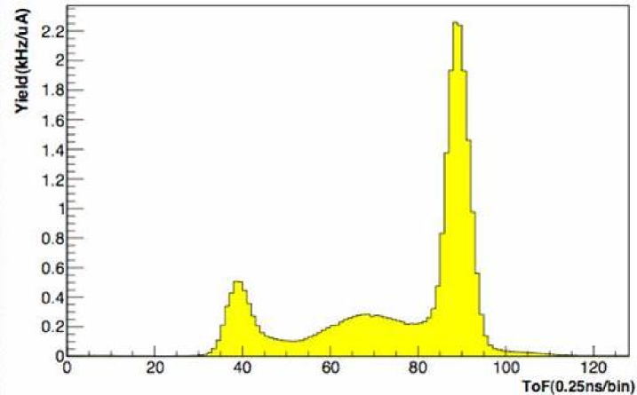
Figure 7: Experimental yield as a function of tof for detector 8. The elastic protons correspond to the rightmost peak.

5 Results

5.1 Time-of-flight spectra

Two calculations are performed without and with RC:

- in the first case, the time-of-flight of elastically scattered protons, without any energy loss nor radiative corrections is calculated. The width of the peak is essentially given by the experimental resolution as calculated by GEANT. The elastic peak is fitted with a Gaussian allowing to determine the position of the maximum, in order to define cuts within which the asymmetry is calculated. The resulting spectra are shown in Fig. 8, where only detector 8, corresponding to the middle of the focal plane, is shown for reference. The only difference in the two spectra is a binning of 250 ps for the French (FR) electronics (top) and a binning of 1 ns for the North-American (NA) electronics (bottom).

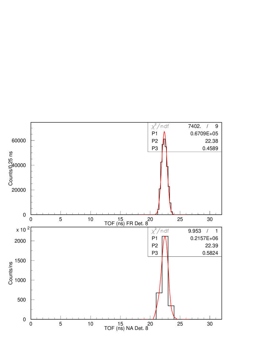
Figure 8: Simulated elastic-proton time-of-flight distributions for Det. 8 (top: FR, bottom: NA). The gaussian fits are performed to extract the position of the mean.

- in the second case, the proton tof spectra are calculated after applying energy losses and full RC. The result obtained for detector 8 is shown in red (grey) in Fig. 9, overlaid to the pure elastic spectra (in black).

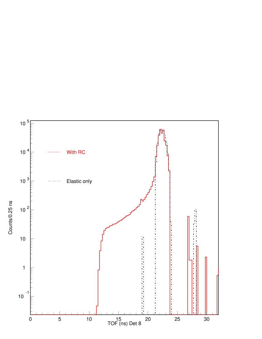
Figure 9: Comparison of time-of-flight spectra (FR Det. 8) without (black dash-dotted line) and with (red/grey solid line) radiative corrections.

One should notice the following paradox: Inelastic protons have, by definition, an energy lower than elastic protons and therefore, a smaller velocity. They should then appear on the right side of the elastic proton peak, corresponding to a longer time-of-flight. In fact, due to the effect of the magnetic field and to the geometry of the $G^{0}$ collimators, inelastic protons have a shorter trajectory and they reach a given detector faster than the elastic ones. This is confirmed in the experimental data.

5.2 Asymmetries

The asymmetry is calculated using Eq. (2). with the following numerical values mus94 :

${\sin}^{2}{\theta}_{{}_{W}}=0.23117$

${G}_{F}=1.16639\times 10^{-5}$

$\mbox{$R_{{}_{V}}^{{}^{p}}$}=-0.0520$, $\mbox{$R_{{}_{V}}^{{}^{n}}$}=-0.0143$, $\mbox{$R_{{}_{V}}^{{}^{(0)}}$}=0$.

$G_{{}_{E}}^{{}^{{\scriptstyle s}}}$ and $G_{{}_{M}}^{{}^{{\scriptstyle s}}}$ are parametrized with a dipole form according to mus94 . A discussion of the latest electromagnetic form factors can be found in arm05 . The strangeness content parameters are from Hammer et al. hmd96 with $\mu_{s}=-0.24$ and $\rho_{s}=-2.93$. These values have been taken from a review paper by Kumar and Souder ks00 . These parameters are used here only as an example of a strange asymmetry calculation. Electromagnetic radiative corrections are rather insensitive to the electroweak parameters. Detailed calculations will be shown on the FR detectors spectra only. Fig. 10 shows the asymmetry distribution without (black line) and with RC (red/grey line). In the elastic case, the asymmetry reduces to the one calculated from the Born term only, and it can be compared directly to theoretical models.

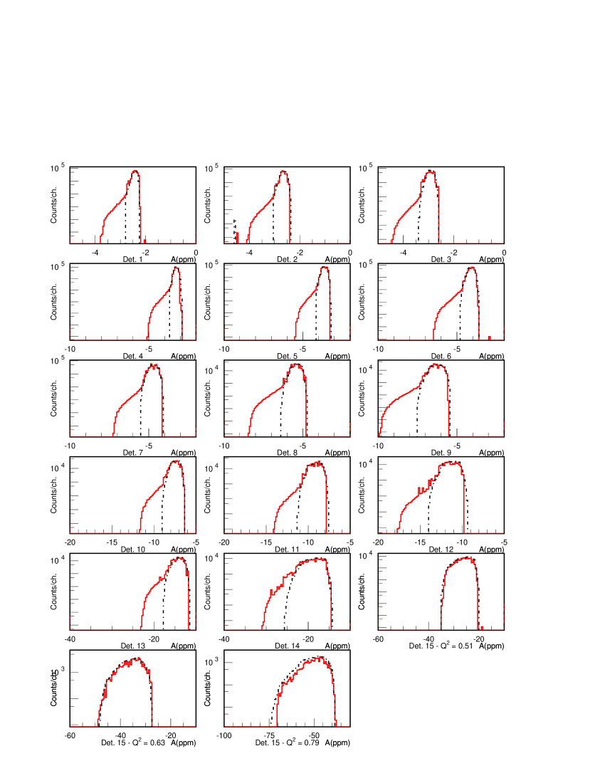
Figure 10: Asymmetry distributions (in ppm), for each detector. The black dash-dotted line represent the elastic case, the red (grey) solid one the radiative case.

The mean asymmetry value is plotted in Fig. 11 for the FR detectors.

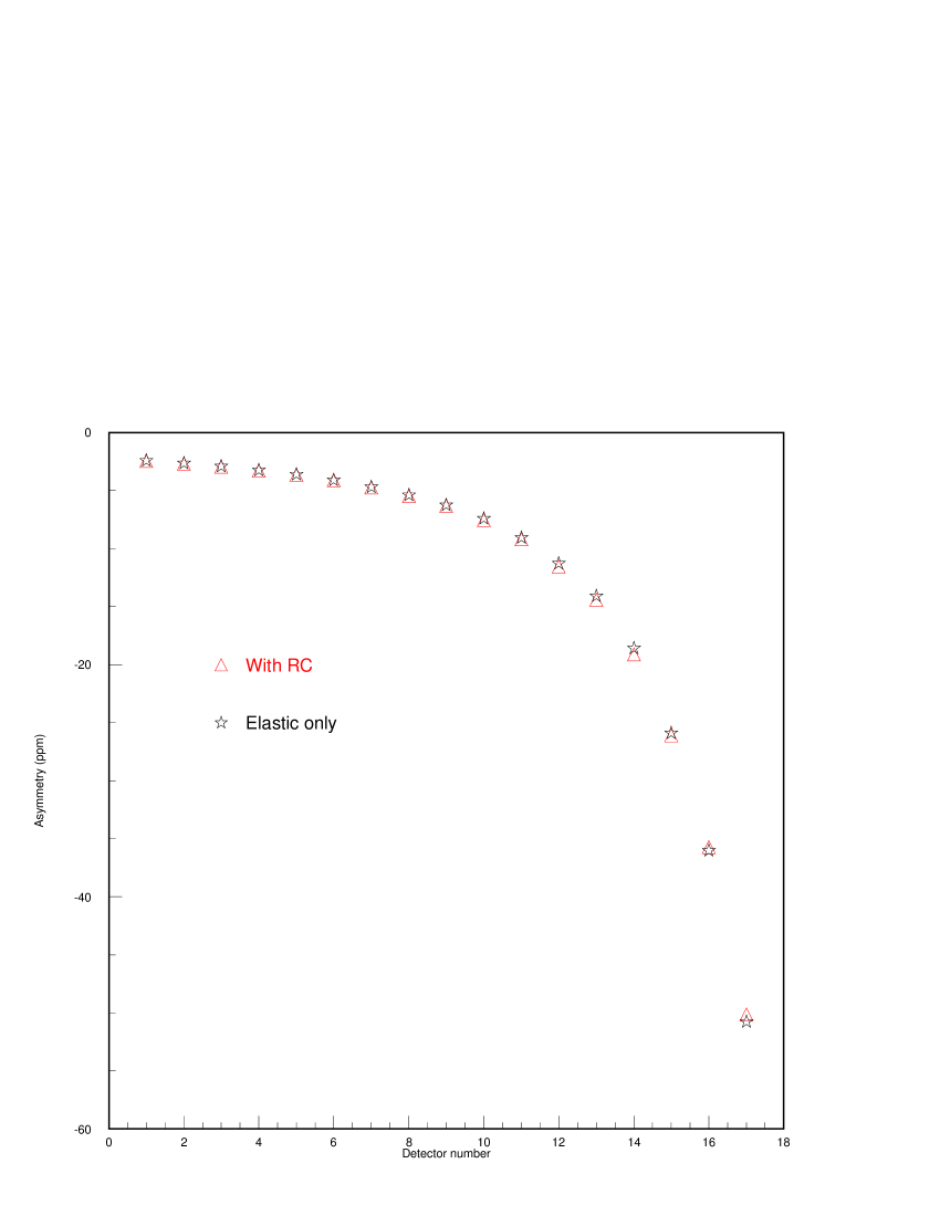
Figure 11: Mean value of the asymmetry for each detector. The black stars represent the elastic case, the red (grey) triangles the radiative one. The “french cuts” on the tof distributions have been applied.

The effect of radiative corrections is to increase the average asymmetry, following the increase in $Q^{2}$. The ratios between elastic and RC corrected asymmetries are given in the following Table 1.

Table 1: Ratio of asymmetries $A_{el}/A_{RC}$ as a function of detector number where $A_{el}$ is the elastic (Born term) asymmetry and $A_{RC}$ is the asymmetry corrected for radiative emission.

Detector #	Ratio
1	0.9971380
2	0.9898130
3	0.9912670
4	0.9911590
5	0.9933250
6	0.9964800
7	0.9915390
8	0.9881630
9	0.9910010
10	0.9828710
11	0.9871740
12	0.9790010
13	0.9767610
14	0.9725560
15/1 $Q^{2}=0.51$	0.9922500
15/2 $Q^{2}=0.63$	1.008340
15/3 $Q^{2}=0.79$	1.012570

The ‘ideal’ procedure to analyze the data would be to calculate an experimental asymmetry from the data after removing all background, leaving an experimental peak including radiative emission, and then to multiply the corresponding asymmetry by the ratio $A_{el}/A_{RC}$ given below. One problem is that, when removing background using a pure fitting procedure, one removes also part of the inelastic tail and therefore, by using the above procedure, one will overestimate the radiative corrections. A quantitative estimate of this effect is given below.

The asymmetry increase is of the order of 0.5-1.0 % for detectors 1-9, reaching 2.0 % for detector 12% and up to 3.0% for detector 14. These ratios should be almost independent of the model chosen and therefore valid for the no-strangeness value A₀. It is not clear if the dispersion between correction factors between 2 adjacent detectors (e.g. between Det. 8-9-10 or 10-11-12), which is of the order of 0.3 %, is an indication of the present statistical/systematical errors or if it is a genuine effect due to differences in acceptance.

5.3 Uncertainty estimate

An error estimate is made based on the assumption that the elastic cuts have a 10% uncertainty. Therefore the radiative corrections are calculated for cuts which are 5% larger than the elastic cuts (by increasing the upper limit by 2.5% and decreasing the lower limit by 2.5%) and 5% smaller than the elastic cuts (by decreasing the upper limit by 2.5% and increasing the lower limit by 2.5%). Then we take the ratio of these two quantities for each detector. This should represent an upper limit of the radiative correction uncertainties since the elastic cuts are known to better than 10%. The corresponding uncertainty would vary slowly from 0.1% for Det. 1 to 0.5% for Det. 13, 1% for Det. 14 and between 0.0% and 0.7% for Det. 15, depending on the $Q^{2}$ cut. An alternative error estimate is obtained by making a global fit of the ratio $A_{el}/A_{RC}$ with a polynomial and assuming that the difference with the actual RC correction is due to systematics: in that case the uncertainty is globally estimated to be of the order of 0.1-0.3% or 10% of the actual correction depending on detector number.

Another problem which has been investigated is the one of correction double-counting. If the background under the elastic peak is removed by a pure fitting procedure, it will also contain the RC tail contribution to the peak. Therefore the corresponding elastic asymmetry should not be corrected for RC effects. In order to estimate the sensitivity of the RC corrections, at the border of the elastic peak, we have calculated the RC corrections by adding or removing 1 ns from the elastic cuts. This effect has been estimated to be about 2% of the RC corrections which are themselves of the order of 2%, so that double counting can be neglected at first order.

6 Summary and conclusions

We have calculated the full electromagnetic radiative corrections for elastic ep scattering in leptonic or hadronic variables; a performable code has been constructed to extract the parity-violating asymmetry from the experimental measured asymmetry. The comparison between the simulation results and the data in the kinematic configuration of the PV-A4 experiment validates our procedure. Radiative corrections for the G0 parity-violating elastic scattering experiment have been estimated by feeding our model calculations through a Monte Carlo detector simulation. This code could also be used for the next asymmetry measurement in the backward-angle configuration of G0.

References

• (1) D.B. Kaplan and A. Manohar, Nucl. Phys. B310, 527 (1988).
• (2) K.S. Kumar and P.A. Souder, Prog. Part. Nucl. Phys. 45, S333 (2000).
• (3) M.J. Musolf et al., Phys. Rep. 1, 239 (1994).
• (4) D. H. Beck and B. R. Holstein, Int. J. Mod. Phys. E10, 1 (2001).
• (5) D. H. Beck and R. D. MacKeown, Ann. Rev. Nucl. Part. Sci. 51, 189 (2001).
• (6) E.J. Beise, M. L. Pitt and D. T. Spayde, Prog. Part. Nucl. Phys. 54, 289 (2005).
• (7) T.Ito et al., Phys. Rev. Lett. 92, 102003 (2004).
• (8) D.T. Spayde et al., Phys. Lett. B58, 79 (2004).
• (9) F.E. Maas et al., Phys. Rev. Lett. 93, 022002 (2004).
• (10) F.E. Maas et al., Phys. Rev. Lett. 94, 082001 (2005).
• (11) D.S. Armstrong et al., Phys. Rev. Lett. 95, 092001 (2005).
• (12) K.A. Aniol et al., Phys. Rev. C69, 065501 (2004).
• (13) Y.S Tsai, Phys. Rev. 122, 1898 (1961).
• (14) L.W. Mo and Y.S Tsai, Rev. of Modern Phys. 41, 205 (1969).
• (15) L.C. Maximon, Rev. of Modern Phys. 41, 193 (1969).
• (16) Y.S Tsai, Rev. of Modern Phys. 46, 815 (1974).
• (17) L.C. Maximon and W.C. Parke, Phys. Rev. C61, 045502 (2000).
• (18) Jefferson Lab Experimental proposal PR 05-108.
• (19) A.F. Afanasev et al., Phys. Lett. B514, 269 (2001).
• (20) S. Drell and T.M. Yan, Phys. Rev. Lett. 25, 316 (1970).
• (21) M.K. Jones et al., Phys. Rev. Lett. 84, 1398 (2000).
• (22) A.I. Akhiezer and M.P. Rekalo, Sov. J. Part. Nucl. 3, 277 (1974).
• (23) D. Bardin and N. Shumeiko, Nucl. Phys. B127, 242 (1977).
• (24) L. Hannelius, private communication.
• (25) H. Guler, Thesis, Universit Paris-Sud, Dec. 2003.
• (26) J. Arvieux et al., $G^{0}$-Collaboration internal report, http://g0web.jlab.org/analysislog/Analysis_Notes/ 050711_100102/PV-short-110705.pdf, July 2005.
• (27) S. Eidelman et al., Phys. Lett. B592, 1109 (2004).
• (28) S. Ong, M.P. Rekalo and J. Van de Wiele, Eur. Phys. J. A 6, 215 (1999).
• (29) B. Collin, Thesis, Université Paris-Sud, Nov. 2002.
• (30) L. Capozza, PAVI04, Eur. Phys. J. A 24, s2, 65 (2005).
• (31) M. Vanderhaegen et al., Phys. Rev. C62, 025501 (2000).
• (32) P. Roos et al, Eur. Phys. J. A 24, 59 (2005) and in preparation for Nucl. Instrum. Meth.
• (33) M. Poelker et al., AIP Conf. Proc. 570, 943, (2001).
• (34) M. Hauger et al., Nucl. Instrum. Meth. A462, 382, (2001).
• (35) J. Van de Wiele and M. Morlet, PAVI04, Eur. Phys. J. A 24, s2 137 (2005).
• (36) H.W. Hammer, U.G. Meissner and D. Drechsel, Phys. Lett. B367, 323 (1996).