POMERON LOOPS IN HIGH ENERGY QCD

Abstract

We discuss the QCD evolution equations governing the high energy behavior of scattering amplitudes at the leading logarithmic level. This hierarchy of equations accommodates normal BFKL dynamics, Pomeron mergings and Pomeron splittings. Pomeron loops are built in the course of evolution and the scattering amplitudes satisfy the unitarity bound.

11.15.Kc, 12.38.Cy, 13.60.Hb

SACLAY–T05/182
ECT*–05–18

1 Introduction

Over the last three decades, one of the main active fields of research within QCD has been the study of its behavior in the high energy limit. In general, a scattering process will be considered as a high energy one, when the (square of the) total energy $s$ of the colliding (hadronic) objects is much larger than the momentum transfer $Q^{2}$ between them. At the same time one hopes to approach the problem via analytical methods, since in this limit there is the possibility of a large kinematical window $s\gg Q^{2}\gg\Lambda_{{\rm QCD}}^{2}$ where one can apply weak coupling methods.

The first approach to the problem was done in the mid seventies when the BFKL (Balitsky, Fadin, Kuraev, Lipatov) equation [1], one of the central equations governing the approach to high energy, was derived. It was understood that certain Feynman diagrams in perturbation theory are enhanced by logarithms of the energy and therefore they have to be resummed. This equation was solved in a special case (for the forward amplitude), and a total cross section growing as a power of the energy emerged. This growth may not be so surprising (at least) a posteriori, since at high energies the wavefunction of a hadron can contain a large number of partons, mainly gluons, due to the available phase space for virtual fluctuations and due to the triple-gluon coupling in QCD. In general, QCD at high energy will be characterized by high densities and increasing (but constraint) cross sections.

Afterwards, in the early to mid eighties, it was realized that one needs to find a mechanism to tame the too steep increase of the partonic densities as predicted by the BFKL equation and the concept of saturation was introduced as a dual description of unitarity in high energy scattering. The gluon density at a given momentum should never exceed a value of order $\mathcal{O}(1/\alpha_{s})$ and, as the mechanism to fulfill this saturation bound, a non-linear term was proposed [2] to be added to the (linear) BFKL equation. Later on a proof of that equation in a special limit (the double logarithmic limit, which nowadays is known not to be a good approximation for a high density system) was given [3]. At the same time another step of progress was made, as the solution of the BFKL equation for non-forward scattering, or equivalently at fixed impact parameter, was obtained [4].

In the mid nineties, one can say that there was a major breakthrough. It was also the time when various subfields were created, as different approaches to address and approach the high energy problem started to develop. The color dipole picture [5, 6, 7, 8] was formulated as a description for the wavefunction of an energetic hadron, a picture which goes beyond the BFKL equation in the sense that it also contains transitions between different number of Pomerons in the multi-color limit (with a Pomeron defined, more or less, as the object which evolves with energy according to the BFKL equation). This allowed one to calculate higher moments of the gluon densities while at the same time the approach to unitarity limits could be studied. A program to calculate the vertices for these Pomeron transitions (beyond the large-$N_{c}$ limit) was started in [9]. Roughly at the same time a somewhat different problem was studied, namely the saturation of densities in the wavefunction of a fast moving large nucleus, due to the strong coherent classical fields generated by the large number of its valence partons [10]. Even though there was no QCD evolution in that model, the ideas introduced proved of great significance for what followed in the forthcoming years. Moreover, that period faced the first attempts to attack the high energy problem by the method of effective actions [11, 12, 13]. Finally a Hamiltonian, equivalent to an integrable system, was given for a particular configuration of $n$ “reggeized” gluons [14, 15].

Even more progress was seen during the last years of the previous decade and the beginning of the current one. The idea introduced earlier in [10] that the wavefunction of an energetic hadron can be described in terms of strong classical color fields, was used properly in order to derive an equation describing the evolution to higher and higher energies. This functional equation, called the JIMWLK (Jalilian-Marian, Iancu, McLerran, Weigert, Leonidov, Kovner) equation [16, 17, 18, 19], gives the evolution of the probability to find a given configuration of a color field associated with the hadronic wavefunction. In general, the physical system which is supposed to be described by such an equation, like a fast moving proton, nucleus or a quarkonium, was called a Color Glass Condensate (CGC) [17], for reasons to be explained later. In turn, the JIMWLK equation can be used to derive equations for the scattering amplitudes of given projectiles off the evolved hadron, and the outcome is what is known by today as the Balitsky hierarchy [20]. This is a set of non-linear equations, which under a mean field and/or large-$N_{c}$ approximation collapses to a single one [21] giving the evolution of the amplitude for a color dipole to scatter off the CGC. As a byproduct, the odderon problem (scattering with an odd number of gluon exchanges) introduced in the early eighties [22, 23, 24] was reformulated and extended to its non-linear version [25, 26]. During that period another important accomplishment was the calculation of the next to leading order correction to the BFKL equation, which was finally completed in [27, 28], while there was an effort to calculate the vertices for Pomeron transitions, their properties and consequences [29, 30, 31, 32, 33], a task which is still ongoing.

Until the beginning of the last year it was thought, at least in some part of the “high energy community”, that the JIMWLK equation was a more or less “complete” and self-consistent description of the high energy limit of QCD (at the leading logarithmic level). However, a calculation done within the dipole picture resulted in some large corrections [34] for the saturation momentum (the momentum scale at a given energy at which gluonic modes saturate). This result was clearly different from what was known up to that time, and the discrepancy was initially attributed to the difference between the JIMWLK equation and its mean field version. Shortly it was understood that these corrections are an effect of the low density fluctuations in the dilute, high-momentum, tail of the wavefunction [35] and in fact the significance of these fluctuations in the evolution of the system had been also observed and realized much earlier from numerical simulations within the dipole picture [36, 37]. The understanding that the JIMWLK equation does not describe properly the low density region of the hadronic wavefunction came soon [38, 39], and a generalization of the Balitsky equations at large-$N_{c}$ was given. This new hierarchy does not allow any kind of mean field approximations and contains loops of Pomerons, in contrast to the Balitsky-JIMWLK one which contains only “one-way” Pomeron transitions. And in fact, the possibility to allow for the formation of Pomeron loops in the course of evolution is of crucial importance for a self-consistent approach to unitarity. Not surprisingly, within this QCD description and under certain logical approximations, the results in [34, 35] were reproduced. Triggered by these observations, facts and derivations, there has been an ongoing effort to the direction of constructing a Hamiltonian formulation and a generalization of the equations at finite-$N_{c}$ [40, 41, 42, 43, 44, 45].

In these lectures we will start by introducing in the next section the BFKL Pomeron and the BFKL equation in coordinate space as was derived in the dipole picture. In Sec. 3 we will discuss its pathologies and in Sec. 4 the concepts of saturation and Pomeron mergings will be proposed as the resolution to the problem, while at the same time a non-linear equation will naturally emerge. In Sec. 5 the Color Glass Condensate, the JIMWLK equation and the Balitsky equations will be presented, and in Sec. 6 the calculation for the energy dependence of the saturation momentum within this formulation will be given. In Secs. 7 and 8 we will try to explain which are the main problems encountered within the JIMWLK evolution and which is the most crucial missing element. In Sec. 9 the dipole picture will be reviewed and the significance of fluctuations will be stressed, while in Secs. 10 and 11 the new hierarchy will be derived, and then the way Pomerons loops are generated will be quite obvious. In the next three sections we will discuss the approach to formulate the problem at the Hamiltonian level, a remarkable (possible) property of the Hamiltonian and the approach to the generalization of the theory beyond the multi-color limit. In the last section the saturation momentum will be revisited, since its energy dependence will be influenced by the low density behavior of the effective theory. As it is clear the presentation will be mostly based on the dipole picture and the Color Glass Condensate formulation of the high energy problem, and over the years there have been nice lectures and reviews for both approaches [46, 47, 48, 49, 50, 51, 52, 53, 54, 55, 56]. We shall not discuss at all any phenomenological aspects of the theory and the possible importance of high density phenomena in the relevant experiments. Nevertheless, we need to say that there have been successful qualitative and sometimes quantitative descriptions of the the low-$x$ data in deep inelastic lepton hadron scattering (DIS) [57, 58, 59, 60] and of the observed particle spectra in heavy-ion collisions [61, 62, 63, 64, 65, 66, 67, 56].

2 The BFKL Pomeron and the BFKL Equation

We start these lectures by introducing the concept and the significance of the BFKL Pomeron and by giving a heuristic, but also intuitive, derivation of the BFKL equation. Imagine that we want to measure the gluon distribution of a generic hadron. One way to do this, is by probing the hadron with a small, in size, color dipole. If the dipole has a size $r=|\bm{x}-\bm{y}|\ll\Lambda_{{\rm QCD}}^{-1}$, where $\bm{x}$ and $\bm{y}$ are the coordinates of its quark and antiquark legs respectively, it will probe the gluonic components of the hadron with momenta such that $Q\sim 1/r\gg\Lambda_{{\rm QCD}}$. Clearly, the condition that the dipole be small, is dictated by the requirement that the QCD coupling constant be small and thus the problem can be approached by analytical methods. Such a probe is not only a good theoretical object due to its overall color neutrality, but it can also be “created” as a fluctuation of the virtual photon in deep inelastic lepton-hadron scattering (DIS). Therefore, if one is able to calculate the dipole-hadron scattering amplitude, one can obtain the cross section for DIS, since the probability for the creation of the dipole is determined by a lowest order calculation in QED. The latter can be easily performed [68] and therefore we shall restrict ourselves to the analysis of the dipole-hadron scattering.

Let us assume that the hadron, to which we shall frequently refer as the target, is right-moving, while the projectile dipole is left moving. We shall also assume that the target is energetic enough, so that a partonic description of its wavefunction is meaningful, while the dipole is slow enough so that it is “bare”; that is, there are no additional components, through higher order radiative corrections, in the dipolar wavefunction.

At lowest order in QCD perturbation theory the dipole and the hadron will interact via a two-gluon exchange as shown in the left part of Fig. 1. Now let the hadron be boosted at very high energy and let $p^{+}$ be the (light-cone) longitudinal momentum of a “valence” parton of the hadronic wavefunction. Then, and as we show in Appendix A in more detail, the probability to emit a soft gluon with longitudinal momentum in the interval from $k^{+}$ to $k^{+}\!+{\rm d}k^{+}$, with $k^{+}=xp^{+}\ll 1$, is proportional to $\alpha_{s}\,{\rm d}k^{+}\!/k^{+}=\alpha_{s}\,{\rm d}x\!/x$. When $x$ is small enough and due to the QCD triple-gluon coupling, the gluon with momentum fraction $x$ can be generated through the intermediate emission of one or more gluons which have their longitudinal momenta strongly ordered, i.e. they satisfy $x\ll x_{n}\ll\dots\ll x_{1}\ll 1$, where $x_{\imath}$ is the momentum fraction of the $\imath$-th gluon in this sequence of emissions of $n$ intermediate gluons. This process, when compared to the direct emission of the soft gluon at $k^{+}$ from the valence parton at $p^{+}$, is of order

$$\alpha_{s}^{n}\int\limits_{x}^{1}\frac{{\rm d}x_{1}}{x_{1}}\,\,\dots\!\int\limits_{x}^{x_{n-1}}\frac{{\rm d}x_{n}}{x_{n}}=\frac{1}{n!}\,\left(\alpha_{s}\ln\frac{1}{x}\right)^{n},$$ (1)

where the logarithms have been clearly generated from the integration over the available longitudinal phase space for the intermediate emissions. At high energies, the rapidity $Y$, defined as $Y=\ln(1/x)$, can compensate the smallness of the coupling $\alpha_{s}$, so that $\alpha_{s}Y\gtrsim 1$. Thus one needs to resum all these $(\alpha_{s}Y)^{n}$ enhanced terms and such a resummation gives rise to the so-called BFKL Pomeron. It is obvious in Eq. (1), that this procedure will lead to an exponential, in $Y$, increase of the gluon density and this will be verified shortly and in more detail when we also take into account the degrees of freedom in the transverse phase space. The interaction of an energetic hadronic target with a color dipole is shown on the right part of Fig. 1, where the summation over the gluon ladder represents the BFKL Pomeron or equivalently the small-$x$ components of the hadronic wavefunction. Notice that this figure corresponds already to the square of a diagram in perturbation theory, since we are interested in determining the probability to find a given mode inside the hadronic wavefunction.

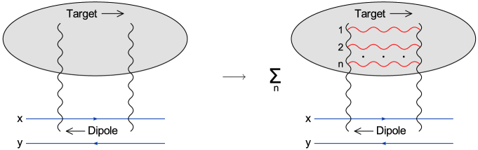
Figure 1: From lowest order in pQCD to the BFKL Pomeron.

Instead of performing the resummation of diagrams, one can equivalently study the evolution of the target wavefunction or of the scattering amplitude under a step $\Delta Y$ in rapidity. Furthermore, one can also view the last soft gluon as being emitted from the projectile dipole, which is a simple object and therefore its evolution can be easily studied. In the large-$N_{c}$ limit the soft gluon can be represented by a quark-antiquark pair, and thus the final system is composed of two dipoles $(\bm{x},\bm{z})$ and $(\bm{z},\bm{y})$, with $\bm{z}$ the transverse coordinate of the emitted soft gluon. As we show in Appendix A the differential probability for this splitting process is [5]

$${\rm d}P=\frac{\bar{\alpha}_{s}}{2\pi}\,\frac{(\bm{x}-\bm{y})^{2}}{(\bm{x}-\bm{z})^{2}(\bm{z}-\bm{y})^{2}}\,{\rm d}^{2}\bm{z}\,{\rm d}Y\equiv\frac{\bar{\alpha}_{s}}{2\pi}\,\mathcal{M}_{\bm{x}\bm{y}\bm{z}}\,{\rm d}^{2}\bm{z}\,{\rm d}Y,$$ (2)

where $\bar{\alpha}_{s}=\alpha_{s}N_{c}/\pi$, with $N_{c}$ the number of colors. In the above equation, ${\rm d}Y={\rm d}\ln(1/x)=-{\rm d}k^{+}/k^{+}$ represents the differential enhancement in the longitudinal phase space as shown in detail in Appendix A, while the kernel $\mathcal{M}_{\bm{x}\bm{y}\bm{z}}$ contains all the QCD dynamics in the transverse phase space. Now, each of the two final dipoles can scatter off the target and therefore the evolution equation for the imaginary part of the scattering amplitude $T$ reads

$$\frac{\partial\langle T_{\bm{x}\bm{y}}\rangle}{\partial Y}\Big{|}_{\rm BFKL}\!=\frac{\bar{\alpha}_{s}}{2\pi}\!\int\limits_{\bm{z}}\!\mathcal{M}_{\bm{x}\bm{y}\bm{z}}\left[\langle T_{\bm{x}\bm{z}}\rangle+\langle T_{\bm{z}\bm{y}}\rangle-\langle T_{\bm{x}\bm{y}}\rangle\right]\equiv\bar{\alpha}_{s}\mathcal{K}_{\rm BFKL}\!\otimes\langle T_{\bm{x}\bm{y}}\rangle,$$ (3)

where the last term is the virtual contribution arising from the normalization of the dipole wavefunction, and with the average to be taken over the target wavefunction, even though this is irrelevant for the moment. This is the BFKL equation [1] in coordinate space [5, 69] and its diagrammatic representation is shown in Fig. 2. It is free of any divergencies, since the potential singularities arising from the poles of the dipole kernel cancel. For example, when $\bm{z}=\bm{x}$ the last two terms in the square bracket cancel each other, while the first term vanishes due to color transparency. In Appendix C we give a more rigorous derivation of Eq. (3), by using the corresponding BFKL equation for the density of dipoles which is derived in Sec. 9.

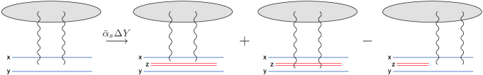
Figure 2: The BFKL equation for the dipole-hadron scattering amplitude.

The BFKL equation is a linear one, and therefore the solution can be obtained by studying the corresponding eigenvalue problem. Let us first look at the simplified case where the scattering amplitude is integrated over the impact parameter $\bm{b}\equiv(\bm{x}+\bm{y})/2$ to give the total cross section, and is invariant under rotations in $\bm{r}$. Then it depends only on the magnitude $r\equiv|\bm{x}-\bm{y}|$ of the projectile dipole. As we show in Appendix D the solution to this eigenvalue problem is

$$\mathcal{K}_{\rm BFKL}\otimes r^{2(1-\gamma)}=\chi(\gamma)\,r^{2(1-\gamma)},$$ (4)

where

$$\chi(\gamma)=2\,\psi(1)-\psi(\gamma)-\psi(1-\gamma),$$ (5)

with $\psi(\gamma)$ the logarithmic derivative of the $\Gamma$-function. The eigenvalue function $\chi(\gamma)$ is plotted in Fig. 3. Thus, one can write the solution to the BFKL equation as the superposition of the evolved with rapidity eigenfunctions, namely

$$\langle T(r,Y)\rangle=\frac{2\pi\alpha_{s}^{2}}{\mu^{2}}\int\limits_{\mathcal{C}}\frac{{\rm d}\gamma}{2\pi{\rm i}}\,T_{0}(\gamma)\exp\left[\bar{\alpha}_{s}\chi(\gamma)Y+(1-\gamma)\ln\left(r^{2}\mu^{2}\right)\right].$$ (6)

In the above equation, $\mu$ is a momentum scale related to the target, the integration contour $\mathcal{C}$ is parallel to the imaginary axis with $0<{\rm Re}(\gamma)<1$, and $T_{0}(\gamma)$ is proportional to the Mellin transformation of the initial cross section at $Y=0$. For instance, when we consider dipole-dipole scattering this initial condition is given by Eq. (96) in Appendix B and in this case $T_{0}(\gamma)$ is equal to $1/[2\gamma^{2}(1\!-\!\gamma)^{2}]$.

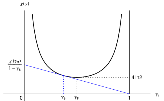
Figure 3: The BFKL eigenvalue $\chi(\gamma)$ as a function of $\gamma_{\rm r}$ when $\gamma_{\rm i}=0$, with $\gamma=\gamma_{\rm r}+{\rm i}\gamma_{\rm i}$. The single poles at $\gamma=0,1$ correspond to the collinear (double logarithmic) limits. The saddle point for the Pomeron intercept occurs at $\gamma_{\mathbb{P}}=1/2$, while $\gamma_{s}=0.372$ corresponds to the relevant anomalous dimension for saturation (see Sec. 6).

At high energies, i.e. when $Y\to\infty$, and with the dipole size $r$ being fixed, one can perform a saddle point integration in Eq. (6). The saddle point of the $\chi$-function occurs at $\gamma_{\mathbb{P}}=1/2$, with corresponding value $\chi(1/2)=4\ln 2$ as shown in Fig. 3, and then the dominant asymptotic energy dependence of the amplitude is given by

$$\langle T\rangle\sim\alpha_{s}\langle\varphi\rangle\sim\alpha_{s}^{2}\langle n\rangle\sim\alpha_{s}^{2}\exp[\omega_{\mathbb{P}}Y],$$ (7)

where $\omega_{\mathbb{P}}=4\bar{\alpha}_{s}\ln 2$ is the so-called hard Pomeron intercept. In Eq. (7), $\varphi$ represents the gluon density of the hadron, while $n$ will be its dipole density if we assume that it is composed of dipoles and this is the case in the large-$N_{c}$ limit. The exponential increase is not surprising, since the BFKL equation is a linear one; in each step of the evolution, the change in the amplitude is proportional to its previous value. After all, this is what we had already expected from the summation of the series whose $n$-th term is given in Eq. (1). Notice also that, even though this is not explicitly written in Eq. (7) but easily inferred from Eq. (6), the dominant $r$-dependence of the amplitude will be proportional to $r$. This is to be contrasted with the result of fixed order perturbation theory which is proportional to $r^{2}$. The fact that the anomalous dimension differs from this perturbative result by a finite pure number is a unique characteristic feature of BFKL dynamics.

The BFKL equation has also been solved in its most general case, i.e. without assuming rotational symmetry and for a given, but arbitrary, impact parameter [4]. In that case the system evolves “quasi-locally” in impact parameter space, and therefore the dominant energy dependence of the solution, as $Y\to\infty$ and with $\bm{r}$ and $\bm{b}$ fixed, is still given by Eq. (7), since the same eigenvalue dominates the corresponding integration.

3 Pathologies of the BFKL Equation

There are two major problems associated with the BFKL equation. The first is the violation of unitarity bounds. As we saw in Sec. 2 the amplitude at a fixed impact parameter increases exponentially with the rapidity $Y$, or equivalently as a positive power of the total energy $s$ in the process, since $Y=\ln(s/s_{0})$ (the precise value of the scale $s_{0}$ is not important for our arguments). However, it should satisfy the unitarity bound

$$T(\bm{r},\bm{b})\leq 1.$$ (8)

One should stress that this bound is different from the well-known Froissart bound [70, 71, 72, 73], which states that any hadronic total cross section $\sigma_{\rm tot}$ should not grow faster than the square of the logarithm of the energy, more precisely

$$\sigma_{\rm tot}\leq\frac{\pi}{m_{\pi}^{2}}\,\ln^{2}s,$$ (9)

with $m_{\pi}$ the pion mass. Of course we should not expect to satisfy this bound by weak coupling methods. The BFKL equation, and all the equations that we will present later on in this article, will never treat properly the “edges” of the hadron, where long range forces become important and therefore the problem is genuinely non-perturbative. Nevertheless, there is no reason a priori which would imply that Eq. (8) cannot be fulfilled in perturbation theory. Notice that Eq. (8) is equivalent to the condition that the maximal allowed gluon density in QCD should be of order $1/\alpha_{s}$. Indeed, one has,

$$\varphi\sim a^{{\dagger}}a\sim A^{2}\lesssim\frac{1}{g^{2}}\sim\frac{1}{\alpha_{s}},$$ (10)

where $a^{{\dagger}}$ and $a$ are gluonic creation and annihilation operators, while $A$ is the gauge field associated with the wavefunction of the hadron. This maximal value of order $1/\alpha_{s}$ can be obtained in a heuristic way by setting the cubic and the quartic in $A$ terms in the QCD Lagrangian to be of the same order.

The second problem is the sensitivity to non-perturbative physics. As already said, the longitudinal momenta are strongly ordered in the course of the evolution. However the transverse coordinates of the dipoles (or equivalently the transverse momenta of the gluons) are not strongly ordered, and therefore the dipole kernel is non-local as clearly seen in Eq. (2). This non-locality results in a diffusion factor which accompanies the dominant asymptotic behavior given in Eq. (7), and which can be easily obtained by performing the Gaussian integration over $\gamma$ in Eq. (6) around the saddle point $\gamma_{\mathbb{P}}=1/2$. This factor reads

$$\psi_{\mathbb{P}}=\frac{1}{\sqrt{\pi D_{\mathbb{P}}Y}}\,\exp\left[-\frac{\ln^{2}(r^{2}\mu^{2})}{D_{\mathbb{P}}Y}\right],$$ (11)

with $D_{\mathbb{P}}=2\bar{\alpha}_{s}\chi^{\prime\prime}(1/2)=56\bar{\alpha}_{s}\zeta(3)$. The form of the function $\psi_{\mathbb{P}}$ suggests that it can be written as the solution to the one-dimensional diffusion equation. That is, after the dominant exponential behavior has been isolated, the evolution can be viewed as a random walk in $\ln(r^{2}\mu^{2})$. Thus, independently of how small the initial dipole is, and after some critical value of rapidity, there will be diffusion to the infrared; dipoles with sizes bigger than $\Lambda_{{\rm QCD}}^{-1}$ will be created and the weak coupling assumption will not be valid any more. One needs to emphasize that this is true even if we want to calculate the amplitude in the perturbative region. Since the diffusion equation is of second order, one can formulate the problem as a path integral from the initial dipole size to the final one. Then, clearly there are paths which go through the non-perturbative region. In this sense the BFKL equation is not self-consistent.

Before moving to the next section, where we will discuss the solution to these problems, let us mention that the next to leading BFKL equation [27, 28] shares the same pathological features. In that case one resums powers of the form $\alpha_{s}(\alpha_{s}Y)^{n}$, and this procedure gives rise to a contribution of order $\mathcal{O}(\alpha_{s})$ to the Pomeron intercept $\omega_{\mathbb{P}}$, as compared to the leading one.

4 Unitarity, Saturation and Mergings of Pomerons

Let us continue our heuristic approach and try to find out which is the basic element that is missing from the procedure we have followed so far. The first diagram in Fig. 4 shows one of the contributing diagrams to the BFKL equation. As indicated, this is of order $\bar{\alpha}_{s}\Delta Y\mathcal{O}(\alpha_{s}\varphi)$, where the factor $\bar{\alpha}_{s}\Delta Y$ comes from the evolution step, the factor $\alpha_{s}$ comes from the two couplings at the lowest part of the diagram and the factor $\varphi$, the target gluon density, is simply the upper part of the diagram. It is clear that the other two BFKL diagrams, which are not shown here, are of the same order. Following the same reasoning, the second diagram is of order $\bar{\alpha}_{s}\Delta Y\mathcal{O}(\alpha_{s}^{2}\varphi^{2})$, since now there are four vertices at the lowest part, while one also probes the gluon pair density of the hadron. This diagram is suppressed with respect to the BFKL ones when $\varphi\ll 1/\alpha_{s}$, i.e. at low densities, or equivalently when $T\ll 1$ and in that case it can be neglected. However it is equally important in the high density limit, precisely in the region where the unitarity problem of the BFKL evolution appears. Therefore, following this “active” point of view in the projectile evolution as before, i.e. the r.h.s. of the equation contains what we have after the evolution step, we see that we should add to the BFKL equation the term which corresponds to the simultaneous scattering of the two dipoles $(\bm{x},\bm{z})$ and $(\bm{z},\bm{y})$, that is

$$\frac{\partial\langle T_{\bm{x}\bm{y}}\rangle}{\partial Y}\Big{|}_{\rm merge}=-\frac{\bar{\alpha}_{s}}{2\pi}\int\limits_{\bm{z}}\mathcal{M}_{\bm{x}\bm{y}\bm{z}}\,\langle T_{\bm{x}\bm{z}}T_{\bm{z}\bm{y}}\rangle.$$ (12)

The resulting evolution equation is the first Balitsky equation [20]. There are a couple of points which need to be clarified in the above equation. The first is the notation “merge” for this particular term. This comes from the fact that the second diagram in Fig. 4 is equivalent to the third one. The latter corresponds to the evolution of the hadron in a “passive” point of view; now the red gluon is supposed to be emitted in the wavefunction of the target, and the two Pomerons, which existed before the evolution step, merge to give rise to a contribution to the single dipole scattering amplitude. However, one should be very careful about the terminology and the interpretation of this merging process. When the hadron is boosted to higher and higher energies, there is no process which would lead to the “mechanical” recombination of the partons that it is composed of. The term merging corresponds to the $4\to 2$ vertex connecting the upper part of the diagram, the hadron, and the lower part, the dipole.

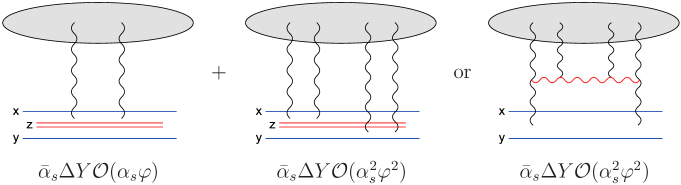
Figure 4: Estimation of diagrams contributing to the first Balitsky equation.

The second point that needs to be explained is the minus sign in Eq. (12). Intuitively, one would indeed expect this term to be negative, since, in almost any physical system, a merging process is supposed to tame the growth of the particle density. A better way to justify the sign, is to notice that we can express the first Balitsky equation in a more compact form, by introducing the $S$-matrix $S_{\bm{x}\bm{y}}=1-T_{\bm{x}\bm{y}}$ (recall that $T$ is the imaginary part of the scattering amplitude). Then we have

$$\frac{\partial\langle S_{\bm{x}\bm{y}}\rangle}{\partial Y}=\frac{\bar{\alpha}_{s}}{2\pi}\,\int\limits_{\bm{z}}\mathcal{M}_{\bm{x}\bm{y}\bm{z}}\left[\langle S_{\bm{x}\bm{z}}S_{\bm{z}\bm{y}}\rangle-\langle S_{\bm{x}\bm{y}}\rangle\right],$$ (13)

which has a clear interpretation; the $S$-matrix for the dipole-pair to scatter off the target multiplied by the splitting probability gives the change in the $S$-matrix for the dipole-hadron scattering (after we subtract the term proportional to $\langle S_{\bm{x}\bm{y}}\rangle$ which gives the survival probability for the parent dipole).

One can proceed and perform certain approximations to this equation. When the target hadron is a large nucleus, and for not too high energies, one can perform a sort of mean field approximation, by assuming that the two projectile dipoles scatter independently off the target, namely

$$\langle T_{\bm{x}\bm{z}}T_{\bm{z}\bm{y}}\rangle\simeq\langle T_{\bm{x}\bm{z}}\rangle\langle T_{\bm{z}\bm{y}}\rangle,$$ (14)

and similarly for the $S$-matrices. Then one obtains a closed equation, the so-called BK (Balitsky, Kovchegov) equation [20, 21] (see also [75]). We immediately notice that this equation has two fixed points; (i) $\langle T\rangle=0\Leftrightarrow\langle S\rangle=1$, which is an unstable fixed point, since no matter how small the initial amplitude is, it will start to grow and (ii) $\langle T\rangle=1\Leftrightarrow\langle S\rangle=0$, which is the black-disk limit, and which is a stable fixed point for any perturbation in $\langle T\rangle$. Therefore the BK equation is much better behaved than the BFKL equation. It seems that the amplitude will never exceed the unitarity bound $T_{\rm max}=1$, and the gluon density will saturate at a value of order $\mathcal{O}(1/\alpha_{s})$. Furthermore the non-linear term cuts all the diffusion to the infrared [76, 77] and there is no sensitivity to non-perturbative physics any more. In fact, all diffusive paths that go beyond the saturation line (see below), will be eliminated by the non-linear evolution.

Here it is appropriate to introduce the concept of the saturation momentum $Q_{s}$. This is a line in the $\ln(r^{2}\mu^{2})\!-\!Y$ plane (in general, the saturation momentum depends also on the impact parameter), along which the amplitude satisfies $\langle T(r=1/Q_{s})\rangle={\rm const}<1$. It is simply the border between the region where BFKL dynamics can be safely applied and the region where saturation has been reached and unitarity corrections have to be taken into account. At this moment, it is not hard to understand that more and more gluonic modes in the wavefunction of the hadron will be saturated, as we keep increasing its energy. As we shall see later on in a detailed analysis, the saturation momentum increases exponentially with rapidity, i.e. $Q_{s}^{2}\approx\Lambda_{{\rm QCD}}^{2}\exp(\lambda_{s}Y)$. Thus, when the rapidity is large enough, one will have $\alpha(Q_{s})\ll 1$, which means that the use of weak coupling techniques is justified. It is conceptually important to realize that this is a “QCD phase” where the physical system is dense but the coupling constant is weak.

By no means we have given a rigorous derivation of the first Balitsky equation in this section. For example, when high density effects become significant, one should not restrict oneself to the two-gluon exchange approximation (even though we didn’t really make any use of it) when considering the scattering of a single dipole with the hadron. Indeed, each coupling of either the quark or the antiquark of the dipole with the classical field $A$ associated with the target is of order $gA\sim\sqrt{\alpha_{s}\varphi}$, and thus in the high density limit $\varphi\sim 1/\alpha_{s}$ all multi-gluon exchanges are equally important. Nevertheless, as we shall see in the next section, the first Balitsky equation remains as given here, even when we include multiple gluon exchanges.

5 The Color Glass Condensate, the JIMWLK Equation and the Balitsky Hierarchy

Perhaps the most elegant, modern and compete approach to describe the merging of Pomerons is the Color Glass Condensate (CGC) and its evolution according to a Renormalization Group Equation (RGE). This is an effective theory within QCD, and its name is not accidental, since it corresponds to some of the basic features that it accommodates. Color stands for the color charge carried by the gluons, Glass stands for a clear separation of time scales between the “fast” and “slow” degrees of freedom in the wavefunction, and Condensate stands for the high density of gluons which can reach values of order $\mathcal{O}(1/\alpha_{s})$.

The essential motivation for the formulation of the CGC is the separation of scales in the longitudinal momenta between the fast partons and the emitted soft gluons. Denoting by $p^{\mu}$ and $k^{\mu}$ the corresponding light-cone 4-momenta, one has $k^{+}\ll p^{+}$. This translates to an analogous separation in light cone energies $k^{-}=\bm{k}^{2}/2k^{+}\gg p^{-}=\bm{p}^{2}/2p^{+}$, which in turn leads to a separation of time-scales; the lifetime $\Delta x^{+}\sim 1/k^{-}$ of the soft gluons will be very short in comparison with the typical time scale $\sim 1/p^{-}$ for the dynamics of the fast partons. Thus, even though the fast partons are virtual fluctuations in reality, they appear to the soft gluons as being a “source” which is $x^{+}$-independent, i.e. as a static source. Furthermore, the source is random, since it corresponds to the color charge seen by the soft gluons at the short period of their virtual fluctuation; this happens at an arbitrary time and it is instantaneous compared to the lifetime of the source. The color charge density $\rho_{a}(x^{-},\bm{x})$ associated with this source at the scale $p^{+}$, propagates along the light cone $x^{-}\simeq 0$ and the corresponding current has just a $+$ component. This source is localized near the light cone within a small distance $\Delta x^{-}\sim 1/p^{+}$, which is non-zero, but much smaller than the longitudinal extent $\sim 1/k^{+}$ of the slow partons. One of the consequences is that the size of the hadron will extend in the longitudinal direction with increasing energy.

Based on the above kinematical considerations, one can represent the fast color sources by a color current $J_{a}^{\mu}(x^{-},\bm{x})=\delta^{\mu+}\rho_{a}(x^{-},\bm{x})$, and the small-$x$ gluons correspond to the color fields as determined by the Yang-Mills equation in the presence of this current, namely

$$\left(D_{\nu}F^{\nu\mu}\right)_{a}(x)=\delta^{\mu+}\rho_{a}(x^{-},\bm{x}).$$ (15)

In principle, and in reality in certain gauges, one can solve this classical equation and obtain the gauge field $A(\rho)$ as a function of a given source. Then, any observable $\mathcal{O}$ which is related to the field, for example the gluon occupation number or the amplitude for an external dipole to scatter off the hadron, can be expressed in terms of $\rho$, and its expectation value will be given by the functional integral

$$\langle\mathcal{O}\rangle=\int\mathcal{D}\rho\,Z_{Y}[\rho]\mathcal{O}(\rho).$$ (16)

It is obvious that $Z_{Y}[\rho]$ serves as a weight measure and it gives the probability density to have a distribution $\rho$ at a given rapidity $Y$ (we assume that $Z_{Y}[\rho]$ is normalized to unity). This probabilistic interpretation for the source relies on its randomness mentioned above; there is no quantum interference between different $\rho$ configurations. In other words, one performs a classical calculation for a fixed configuration of the sources, and then one averages over all the possible configurations with a classical probability distribution.

So far, in Eqs. (15) and (16) we have not used at all the small-$x$ QCD dynamics, and it is obvious that this must be encoded in the probability distribution $Z_{Y}[\rho]$, which is the only quantity in Eq. (16) depending on rapidity. But before analyzing this aspect in more detail, we have to say that this idea to describe the soft modes of the hadronic wavefunction in terms of classical fields and probability densities was introduced in the MV (McLerran, Venugopalan) model [10], where a nucleus with large atomic number ($A\gg 1$) was considered. In this “static” model the only color sources are assumed to be the $A\times N_{c}$ valence quarks, which are taken to be uncorrelated for transverse separations such that $|\Delta\bm{x}|\lesssim\Lambda_{{\rm QCD}}^{-1}$, so that the probability density is given by the Gaussian [10, 78]

$$Z_{\rm MV}[\rho]\approx\exp\left[-\frac{1}{2}\int^{\Lambda^{-1}}\!\!\!\!{\rm d}^{2}{\bm{x}}\,\frac{\rho^{a}(\bm{x})\,\rho^{a}(\bm{x})}{\mu^{2}(\bm{x})}\right],$$ (17)

where $\mu^{2}\sim\Lambda_{{\rm QCD}}^{2}A^{1/3}$ is the average color charge density squared. Even though there is no $Y$-dependence in the model, a strong coherent color field of order $\mathcal{O}(1/g)$ can be created due to the large number of nucleons and the solution of, the non-linear, Eq. (15) will lead to the saturation of the gluon density at a value of order $\mathcal{O}(1/\alpha_{s})$, and with a saturation scale $Q_{s}^{2}(A)\approx\Lambda_{{\rm QCD}}^{2}A^{1/3}\ln A$.

Now let us see how and why the evolution of the probability distribution arises. Indeed, at rapidity $Y$, one should include in the source all those modes with longitudinal momenta (much) larger than $k^{+}$, where $Y=\ln(1/x)=\ln(P^{+}/k^{+})$ with $P^{+}$ the total longitudinal momentum of the hadron. Now let us imagine that we increase the rapidity from $Y$ to $Y+\Delta Y$. Then, some modes that previously were “slow”, now they become “fast” and they need to be integrated over in order to be included in the source. This is a procedure which will crucially depend on the actual QCD dynamics and will lead to a change in the probability distribution. Still, we should emphasize that the theory at the new “scale” $Y+\Delta Y$ is again defined through Eqs. (15) and (16), if we simply let $Y\to Y+\Delta Y$. A simple pictorial interpretation of the evolution with $Y$ of the probability distribution is shown in Fig. 5, where the red gluon at the rapidity $Y^{\prime}$ is a representative of the “semi-fast” modes which are integrated, i.e. $Y\ll Y^{\prime}\ll Y+\Delta Y$.

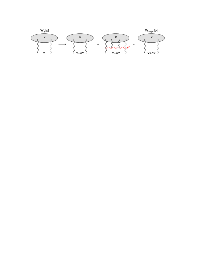
Figure 5: Evolution of the probability distribution of color charges.

We shall not present here the derivation of this RGE, which is called the JIMWLK equation (even though a “sketch” of such a derivation is given in Appendix E). It can be found in the original papers [16, 17, 18, 19] (see also [79, 80]), while rather simple derivations can be found in [81, 44, 55]. The basic element is the resummation of $\bar{\alpha}_{s}\ln(1/x)$ enhanced contributions in the presence of a background color field. The latter is allowed to be strong in general, since one aims to describe properly the physics in the high density region. This equation can be given an elegant Hamiltonian formulation, and its most compact representation arises when it is expressed in terms of the color field $\alpha(x^{-},\bm{x})\equiv A^{+}(x^{-},\bm{x})$ in the Coulomb gauge. It reads

$$\frac{\partial}{\partial Y}\,Z_{Y}[\alpha]=H\left[\alpha,\frac{\delta}{\delta\alpha}\right]Z_{Y}[\alpha],$$ (18)

where the explicit form of the Hamiltonian is [17, 18, 26]

$$H=-\,\frac{1}{16\pi^{3}}\!\int\limits_{\bm{u}\bm{v}\bm{z}}\!\mathcal{M}_{\bm{u}\bm{v}\bm{z}}\left[1+\tilde{V}_{\bm{u}}^{{\dagger}}\tilde{V}_{\bm{v}}-\tilde{V}_{\bm{u}}^{{\dagger}}\tilde{V}_{\bm{z}}-\tilde{V}_{\bm{z}}^{{\dagger}}\tilde{V}_{\bm{v}}\right]^{ab}\frac{\delta}{\delta\alpha^{a}_{\bm{u}}}\,\frac{\delta}{\delta\alpha^{b}_{\bm{v}}}.$$ (19)

The dipole kernel is readily recognized, while the Wilson lines $\tilde{V}$ in the adjoint representation arise from the gluon propagator of the integrated modes and they are given by

$$\tilde{V}^{\dagger}_{\bm{x}}[\alpha]={\rm P}\,\exp\left[{\rm i}\,g\int\limits_{-\infty}^{\infty}{\rm d}x^{-}\alpha^{a}(x^{-},{\bm{x}})\,T^{a}\right].$$ (20)

The longitudinal coordinate in the functional derivatives is to be taken at $\infty$, since $x^{-}\sim 1/k^{+}\sim{\rm e}^{Y}/P^{+}\to\infty$; as we pointed out earlier, the hadron extends in the longitudinal direction, and all the “action” is expected to take place at the last layer of rapidity. Finally, the two functional derivatives appearing in Eq. (19) correspond precisely to the two outgoing legs in the bottom of the diagrams in Fig. 5. The appearance of only two such legs is related to the certain class of diagrams which are effectively resummed by the JIMWLK equation; during a single evolution step, only the two point correlation function $\langle\rho\rho\rangle$ changes, and this comes from the fact that the color field, or equivalently the sources, are assumed to have values (much) larger than $g$. This is certainly a well-defined approximation, but with a decisive influence on the outcomes of the theory. We shall not discuss more details here, but we shall return to this issue and to its proper treatment, in the next sections.

Given a Hamiltonian, the natural question that one may ask is which the observables are. They can be nothing else than the quantities already appearing in the Hamiltonian, and to be more precise, they will be gauge invariant operators built from Wilson lines. For our purposes, we shall only consider Wilson lines in the fundamental representation and then the most generic form of such an operator will read

$$\mathcal{O[\alpha]}={\rm tr}\big{(}V_{\bm{x}_{1}}^{\dagger}V_{\bm{x}_{2}}V_{\bm{x}_{3}}^{\dagger}V_{\bm{x}_{4}}\dots\big{)}{\rm tr}\big{(}V_{\bm{y}_{1}}^{\dagger}V_{\bm{y}_{2}}\dots\big{)}\dots$$ (21)

Notice that a Wilson line has a direct physical interpretation [82]. Let us consider the scattering of a left-moving quark off the classical field created by the (right-moving) hadron. The general expression for the $S$-matrix in the interaction picture is

$$S={\rm T}\exp\left[-{\rm i}\int\limits_{-\infty}^{\infty}{\rm d}^{4}x^{\prime}\,H_{\rm I}(x^{\prime})\right],$$ (22)

where T stands for a time ordered product, and the relevant part of the QCD Hamiltonian for this process is $H_{\rm I}=-g\bar{\psi}\gamma^{-}A^{+}\psi$. Here we have used the fact that the quark is a fast left mover and therefore the $\gamma^{-}$ matrix dominates the inner product. Now, since the trajectory is “eikonal”, the transverse and $+$ coordinates of the particle are fixed, and they are chosen to be $\bm{x}^{\prime}=\bm{x}$, and (by convention) $x^{\prime+}=x^{+}=0$. Therefore, so long as the color independent part is concerned, one can make the substitution

$$\bar{\psi}(x^{\prime})\,\gamma^{-}A^{+}(x^{\prime})\,\psi(x^{\prime})\to\delta(\bm{x}^{\prime}-\bm{x})\,\delta(x^{\prime+}\,)A^{+}(x).$$ (23)

Since $x^{-}$ is increasing along the trajectory, one can replace the T-product by a Path ordered product. Therefore the $S$-matrix is equal to the Wilson line $V_{\bm{x}}^{{\dagger}}$ given in Eq. (20), but in the fundamental representation, i.e. one needs to do the replacement $T^{a}\to t^{a}$. Notice that all kind of multiple exchanges are included in this procedure, and they can be recovered by expanding the Wilson lines to a given order in the coupling constant. It is not hard to understand that the $S$-matrix for a dipole $(\bm{x},\bm{y})$ to scatter off the target will be given by the gauge invariant expression

$$S_{\bm{x}\bm{y}}=\frac{1}{N_{c}}\,{\rm tr}\big{(}V_{\bm{x}}^{\dagger}V_{\bm{y}}\big{)}=1-T_{\bm{x}\bm{y}}=1-\frac{g^{2}}{4N_{c}}(\alpha^{a}_{\bm{x}}-\alpha^{a}_{\bm{y}})^{2}+\mathcal{O}(g^{3}),$$ (24)

where we have also expanded to second order to obtain the scattering amplitude in the two-gluon exchange approximation for later convenience, and with the field $\alpha^{a}$ in this expansion being integrated over $x^{-}$.

As discussed earlier, the evolution of the expectation value of a generic operator $\mathcal{O}$ will come from the evolution of the probability distribution $Z_{Y}[\rho]$. Using Eqs. (16), (18) and (19), and after a functional integration by parts we find

$$\frac{\partial\left\langle\mathcal{O}\right\rangle}{\partial Y}=\int\mathcal{D}\alpha\,Z_{Y}[\alpha]\,H\,\mathcal{O}=\left\langle H\,\mathcal{O}\right\rangle.$$ (25)

Now we are ready to write the equations obeyed by the scattering amplitudes. Naturally, we start from the scattering of a single projectile dipole. Using Eqs. (19), (24) and (25), and as we show explicitly in Appendix F, we arrive at the first Balitsky equation which we rewrite here for convenience

$$\frac{\partial\langle S_{\bm{x}\bm{y}}\rangle}{\partial Y}=\frac{\bar{\alpha}_{s}}{2\pi}\,\int\limits_{\bm{z}}\mathcal{M}_{\bm{x}\bm{y}\bm{z}}\langle S_{\bm{x}\bm{z}}S_{\bm{z}\bm{y}}-S_{\bm{x}\bm{y}}\rangle.$$ (26)

Notice that the above equation is valid for a finite number of colors and the same will be true for the BFKL equation which arises in the limit $\langle T\rangle=1-\langle S\rangle\ll 1$. As we have already discussed, this is not a closed equation and one needs to find how $\langle S_{\bm{x}\bm{z}}S_{\bm{z}\bm{y}}\rangle$ evolves with rapidity. Following the same procedure, and as we show again in Appendix F, one obtains the second Balitsky equation, which reads

$$\frac{\partial\langle S_{\bm{x}\bm{z}}S_{\bm{z}\bm{y}}\rangle}{\partial Y}=\frac{\bar{\alpha}_{s}}{2\pi}\,\int\limits_{\bm{w}} \!\!\!\!\!\!\mathcal{M}_{\bm{x}\bm{z}\bm{w}}\,\langle(S_{\bm{x}\bm{w}}S_{\bm{w}\bm{z}}-S_{\bm{x}\bm{z}})S_{\bm{z}\bm{y}}\rangle$$

$$+\frac{\bar{\alpha}_{s}}{2\pi}\,\int\limits_{\bm{w}} \!\!\!\!\!\!\mathcal{M}_{\bm{z}\bm{y}\bm{w}}\,\langle S_{\bm{x}\bm{z}}(S_{\bm{z}\bm{w}}S_{\bm{w}\bm{y}}-S_{\bm{z}\bm{y}})\rangle$$ (27)

$$\!\!\!\!\!\!+\frac{1}{2N_{c}^{2}}\,\frac{\bar{\alpha}_{s}}{2\pi}\,\int\limits_{\bm{w}}(\mathcal{M}_{\bm{x}\bm{y}\bm{w}}\!-\!\mathcal{M}_{\bm{x}\bm{z}\bm{w}}\!-\!\mathcal{M}_{\bm{z}\bm{y}\bm{w}})\langle Q_{\bm{x}\bm{z}\bm{w}\bm{y}}+Q_{\bm{x}\bm{w}\bm{z}\bm{y}}\rangle,$$

where we have defined the “quadrupole” operator

$$Q_{\bm{x}\bm{z}\bm{w}\bm{y}}\equiv\frac{1}{N_{c}}\left[{\rm tr}\big{(}V^{{\dagger}}_{\bm{x}}V_{\bm{w}}V^{{\dagger}}_{\bm{z}}V_{\bm{y}}V^{{\dagger}}_{\bm{w}}V_{\bm{z}}\big{)}-{\rm tr}\big{(}V^{{\dagger}}_{\bm{x}}V_{\bm{y}}\big{)}\right].$$ (28)

At this point a few comments need to follow. We immediately notice that the first two terms in the second Balitsky equation can be obtained just by applying the Leibnitz differentiation rule to the first Balitsky equation. This has a natural interpretation in terms of projectile evolution as the two dipoles $(\bm{x},\bm{z})$ and $(\bm{z},\bm{y})$ can evolve independently; either of these two dipoles can split into two new dipoles which subsequently scatter off the unevolved target hadron. However, there is the third term which goes beyond this simple dipolar evolution. This is not surprising since the small-$x$ gluon emitted by the one of the two original dipoles can be absorbed by the other dipole (more precisely, emitted by the other dipole in the complex conjugate amplitude when calculating the wavefunction of the projectile) and therefore no dipole survives after the evolution step. Thus, the projectile system is lead to a more complicated multipolar state, which can be naturally called a color quadrupole because of its dependence on four transverse coordinates. For the next step one will have to write not only the evolution equation for the three-dipoles operator, but also the one for this quadrupole operator. It becomes clear that the complexity in the structure of this hierarchy of equations, which is called the Balitsky hierarchy, will rapidly increase as we proceed to describe the evolution of “higher-point” functions. Following this “active” point of view in the projectile evolution, we see that is wavefunction will be successively composed of

$${\rm one\,\,dipole} \!\!\!\!\!\!\,\to\,{\rm two\,\,dipoles}\,\to\,{\rm three\,\,dipoles}\,+\,{\rm quadrupole}$$

$$\!\!\!\!\!\!\,\to\,\dots\,\to\,{\rm dipoles}\,+\,{\rm higher\,\,multipolar\,\,states}.$$

Furthermore, we should emphasize that no factorization like the one in Eq. (14) will solve the infinity hierarchy. Nevertheless, we see that the two fixed points of the BK equation, when generalized properly, satisfy this system of equations. (i) When the classical color field $\alpha^{a}$ vanishes there is no scattering; the expectation values of all the Wilson lines become equal to unity, i.e. $\langle S\rangle=\langle SS\rangle=\langle Q\rangle=\dots=1$ and (ii) when the color field becomes large, we reach the black-disk limit; the Wilson lines oscillate rapidly [83] and their expectation values vanish; i.e. $\langle S\rangle=\langle SS\rangle=\langle Q\rangle=\dots=0$.

One expects drastic simplifications in the large-$N_{c}$ limit where the degrees of freedom can be chosen to be the color dipoles. Indeed, the last (quadrupole) term in Eq. (5) is of order $\mathcal{O}(1/N_{c}^{2})$, negligible at large-$N_{c}$ when compared to the first two (dipolar) terms which are of order $\mathcal{O}(1)$ and therefore the evolution will proceed only through dipolar states. Now one can see that the hierarchy becomes consistent with a factorization of the form [84, 85]

$$\langle S_{\bm{x}_{1}\bm{y}_{1}}\dots S_{\bm{x}_{\kappa}\bm{y}_{\kappa}}\rangle=c^{\kappa-1}\langle S_{\bm{x}_{1}\bm{y}_{1}}\rangle\dots\langle S_{\bm{x}_{\kappa}\bm{y}_{\kappa}}\rangle,$$ (29)

with $c$ an arbitrary constant. Then the whole large-$N_{c}$ hierarchy collapses to a single equation, the BK equation but with a coefficient $c$ in front of the $\langle S_{\bm{x}\bm{z}}\rangle\langle S_{\bm{z}\bm{y}}\rangle$ term. The asymptotic fixed point of this equation is clearly $1/c$, but it is not clear whether a value $c\neq 1$ has a simple physical interpretation or not. In any case, if the initial conditions at a rapidity $Y_{0}$ are of factorized form, this factorization will be preserved by the large-$N_{c}$ evolution. But even if the initial conditions are not of this type, no new “correlations” will be generated by this large-$N_{c}$ evolution; only the initial ones will be propagated to higher rapidities.

6 The Saturation Momentum

With the theory of the Color Glass Condensate being theoretically established, one of the central problems has been the determination of the saturation momentum $Q_{s}$ which, as we discussed at the end of Sec. 4, is the momentum scale at which we start to approach unitarity limits. In principle one should be able to calculate the energy (rapidity) dependence of $Q_{s}$ (at least asymptotically), since all the dynamics is contained in the JIMWLK equation, however its precise value cannot be determined since it will depend on initial conditions and thus on details of non-perturbative physics. Recall that the saturation momentum is an intrinsic property of the target hadron, since it is also the scale where the gluon density saturates. And the only scale associated with the hadron is $\Lambda_{{\rm QCD}}$. Given the above considerations, and the fact that the pure BFKL evolution leads to an exponential growth, one may guess that the saturation momentum will be of the form (for fixed coupling, neglecting the impact parameter dependence and at asymptotic energies)

$$Q_{s}^{2}\simeq c\,\Lambda_{{\rm QCD}}^{2}\frac{\exp(\lambda Y)}{Y^{\beta}},$$ (30)

where the constants $\lambda$ and $\beta$ should be calculable, while the constant $c$ would require the knowledge of the non-perturbative structure of the hadron.

Even though the problem seems difficult at a first sight due to the complicated structure of the Balistky-JIMWLK equations, one can do certain logical simplifications that render the calculation tractable. As we saw, the hierarchy reduces to the much simpler BK equation in the large-$N_{c}$ limit and under a mean-field approximation, and then, presumably, the most that one may lose is $1/N_{c}^{2}$ corrections. Furthermore, one can in fact use BFKL dynamics, if one is careful enough to treat properly the effects of the linear terms. In turn, this means that we may not even lose the possible $1/N_{c}^{2}$ corrections, since the BFKL equation is valid at finite-$N_{c}$.

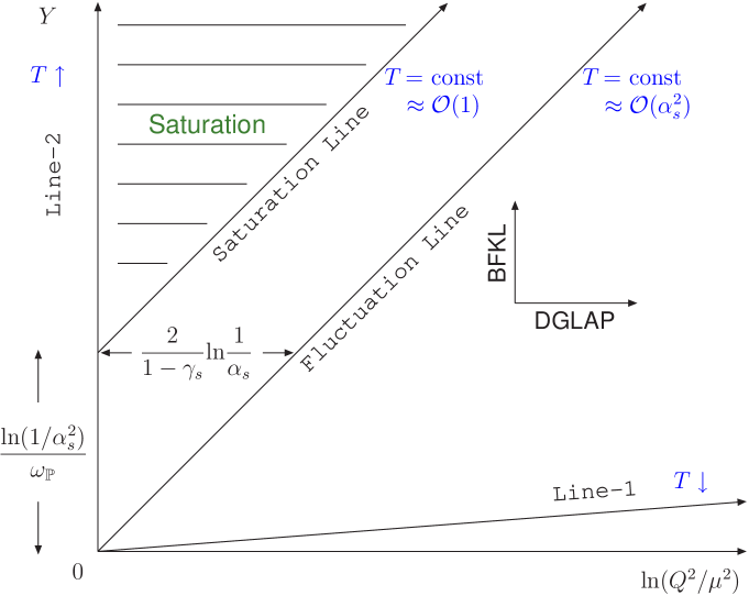
Figure 6: Scattering amplitude and saturation momentum in the logarithmic plane.

Now let us have a look at Fig. 6 where the expected qualitative behavior of the scattering amplitude in the logarithmic plane $\ln(Q^{2}/\mu^{2})-Y$ is shown. Here $Q$ should be thought as the inverse of the dipole size or as the transverse momentum of a gluon in the hadron. Along Line-1, which corresponds to an anomalous dimension $\gamma\to 0$, the amplitude decreases since the momentum increases too fast. This corresponds to DGLAP evolution (in the double logarithmic limit) where one resums powers of $\alpha_{s}\ln(Q^{2}/\mu^{2})$ ($\times\ln(1/x)$). In this case there is again a cascade of partons inside the hadron, but these partons are very small in size and they will never overlap to form a high density system. Along Line-2, which corresponds to an anomalous dimension $\gamma_{\mathbb{P}}=1/2$, the amplitude increases, since the energy increases while the momentum remains fixed. This is the hard Pomeron intercept line and corresponds to the saddle point of the BFKL eigenvalue function. Starting from a value of order $\mathcal{O}(\alpha_{s}^{2})$ and after covering a rapidity interval $\sim\ln(1/\alpha_{s}^{2})/\omega_{\mathbb{P}}$, the amplitude will eventually “hit” the unitarity/saturation region.

Therefore, there must be some “critical” line between those two lines which belongs to the region of linear evolution and along which the amplitude remains constant, for example of order $\mathcal{O}(\alpha_{s})\ll 1$. Clearly this line must correspond to an anomalous dimension, say $\gamma_{s}$, such that $0<\gamma_{s}<1/2$. Then the saturation line which corresponds to constant amplitude of order $\mathcal{O}(1)$ but smaller than 1, for example 1/2, will be parallel to the critical line, and therefore characterized by the same anomalous dimension and energy dependence. The reason why the two lines are parallel, may not be so clear at the moment, but we will try to justify it in a while.

The question is whether or not we can use the BFKL dynamics to determine this critical line. Even though the line belongs to the linear region, the answer is negative if one wants to get the prefactors correct, i.e. the value of $\beta$ in Eq. (30). The reason is that as the system evolves along this line, and after we have isolated the leading exponential behavior, there we will be some paths, really in the functional integral sense, that go through the saturation region and then return to the linear one. These diffusive paths are absent when the full BK equation is equation is considered, and therefore should be cut. This can be done by using an absorptive boundary just beyond the saturation line, which will mimic the effects of the non-linear terms for the problem under consideration. Put it another way, this procedure is equivalent to a self-consistent solution of the BFKL equation with the boundary condition $\langle T(Q=Q_{s}(Y))\rangle=c<1$.

Now we are ready to determine the “slope” of the critical, and therefore of the saturation, line. We impose two conditions for the exponent in the solution to the BFKL equation as given in Eq. (6). First we require the exponent to be zero so that the amplitude be constant. Second we impose a saddle point condition, which is a valid approximation in the asymptotic limit $\bar{\alpha}_{s}Y\gg 1$. Then we find that the anomalous dimension is determined by the saddle-point of $\chi(\gamma)/(1\!-\!\gamma)$ and is given by [2, 86, 87, 77, 88]

$$\chi(\gamma_{s})+(1\!-\!\gamma_{s})\,\chi^{\prime}(\gamma_{s})=0\Rightarrow\gamma_{s}=0.372.$$ (31)

The energy dependence of the saturation momentum is better expressed in terms of its logarithmic derivative which reads [77, 88] (with the leading term already known from [86, 87])

$$\lambda_{s}\equiv\frac{{\rm d}\ln Q_{s}^{2}}{{\rm d}Y}=\bar{\alpha}_{s}\,\frac{\chi(\gamma_{s})}{1\!-\!\gamma_{s}}-\frac{3}{2(1\!-\!\gamma_{s})}\,\frac{1}{Y}=4.88\,\bar{\alpha}_{s}-\frac{2.39}{Y},$$ (32)

while for the scattering amplitude one obtains [77, 88] (and with the absence of the logarithmic modification, already known from [87])

$$\langle T\rangle=\left(\frac{Q_{s}^{2}}{Q^{2}}\right)^{1-\gamma_{s}}\!\!\left(\ln\frac{Q^{2}}{Q_{s}^{2}}+\rm{c}\right)\exp\left[-\frac{\ln^{2}(Q^{2}/Q_{s}^{2})}{D_{s}Y}\right],$$ (33)

a form which is valid in the region $Q_{s}^{2}\ll Q^{2}\ll Q_{s}^{2}\exp(D_{s}Y)$, and where the diffusion coefficient is $D_{s}=2\bar{\alpha}_{s}\chi^{\prime\prime}(\gamma_{s})=97\bar{\alpha}_{s}$.

Now let us discuss the results. As we see in Eq. (31), whose graphical solution is shown in Fig. 3, the relevant value of the anomalous dimension for saturation lies indeed in the interval $(0,1/2)$. We should say that the eigenvalue $\chi(\gamma_{s})$ will be selected, so long as the initial condition contains the corresponding eigenfunction and this will be true for all interesting cases. Notice that $\gamma_{s}$ is a pure number, and this would have never been obtained by applying pure DGLAP evolution. The latter always gives anomalous dimensions which start at order $\mathcal{O}(\alpha_{s})$.

In Eq. (32) we see that the leading contribution to the “intercept” of the saturation line is totally fixed by BFKL dynamics. It is not too difficult to see how the subleading correction arises, and to this end let us go a few steps back in the derivation of Eqs. (32) and (33). After we have performed the Gaussian integration around the saddle point $\gamma_{s}$, the solution reads $T\propto(Q_{0}^{2}/Q^{2})^{1-\gamma_{s}}\psi_{s}$, with $Q_{0}$ containing only the leading behavior of $Q_{s}$, and where $\psi_{s}$ satisfies the diffusion equation. The “standard” solution to the diffusion equation behaves as $Y^{1/2}$ (times the exponential diffusion factor), but in the presence of an absorptive boundary the survival probability of the “particle” becomes smaller and $\psi_{s}$ is proportional to $1/Y^{3/2}$. Thus, by combining this prefactor and the leading behavior $Q_{0}$, one obtains the correction written in Eq. (32). Notice that the saturation effects lead to a slower increase of the saturation momentum, as they should. Even though the second term vanishes when $Y\to\infty$, it cannot be neglected, since upon integration of Eq. (32) it will generate a $Y$-dependent prefactor in $Q_{s}$. This $1/Y$ term in the logarithmic derivative of the saturation momentum should be interpreted as $1/R_{D}^{2}$, where $R_{D}\sim\sqrt{Y}$ is the diffusion radius. This radius is practically the available phase space in logarithmic units of transverse momentum. In reality this phase space extends to infinity, since there is no boundary to the ultraviolet, but in practice it is only the space inside the diffusion radius which will contribute to the subsequent steps of evolution.

Finally, as we see in Eq. (33), the scattering amplitude has a scaling form [87, 77], so long as $\ln(Q^{2}/Q_{s}^{2})\ll\sqrt{D_{s}Y}$ so that the exponential diffusion factor can be set equal to unity. That is, the amplitude does not depend on $Q^{2}$ and $Y$ separately, but only through the variable $Q^{2}/Q_{s}^{2}$. The pure power is not an unexpected result; the BFKL evolution generates the anomalous dimension $\gamma_{s}$ which modifies the behavior $\sim 1/Q^{2}$ of fixed order perturbation theory. The logarithm is generated by the absorptive boundary when solving the diffusion equation. Notice that both terms in Eq. (33), the power and the power modified by the logarithm, are exact degenerate solutions to the BFKL equation [89], and thus the final solution is just their linear combination. Such a scaling behavior, which will be preserved even in the running coupling case (but in a more narrow window in $Q^{2}$), but which will be violated by the evolution equations that we will discuss later on in Sec. 10, is consistent with fits [57, 58, 60] of the low-$x$ data in DIS.

Here it is appropriate to mention that the solution of the BK equation close to the unitarity limit $\Lambda_{{\rm QCD}}^{2}\ll Q^{2}\ll Q_{s}^{2}$ is also of scaling form and as we show in Appendix G it reads [37, 90, 83]

$$\langle S\rangle=1-\langle T\rangle\approx\exp\left[-\frac{1-\gamma_{s}}{2\chi(\gamma_{s})}\,\ln^{2}\frac{Q_{s}^{2}}{Q^{2}}\right].$$ (34)

Thus, one naturally expects the scattering amplitude to satisfy scaling everywhere from deep inside the saturation region up to momenta which belong in the region of linear evolution. This explains why the critical and saturation lines are parallel to each other.

Eqs. (31), (32) and (33) have been confirmed by studying the analogy to the (nonlinear) FKPP (Fisher, Kolmogorov, Petrovsky, Piscounov) equation [91, 88]. Furthermore, the last asymptotic term of $\lambda_{s}(Y)$ which is independent of the initial conditions, and whose behavior is $\sim 1/Y^{3/2}$ has been obtained in the same fashion in [92]. The full JIMWLK hierarchy has been solved numerically on the lattice [93] and the results agree with the ones we presented in this section. Moreover it was found that violations of factorization in the scattering amplitude correlations are extremely small.

Before closing this section, let us see how these results are modified when we consider BFKL dynamics at the next to leading level. The calculation of the next to leading order (NLO) correction to the BFKL kernel was completed in [27, 28]. However, this negative correction turned out to be larger in magnitude than the leading contribution for reasonable values of the coupling, say $\bar{\alpha}_{s}\approx 0.25$. Even worse, when $\bar{\alpha}_{s}\gtrsim 0.05$ the full kernel has two complex saddle points which lead to oscillatory cross sections [94]. But it was immediately recognized that these large corrections emerge from the collinearly enhanced physical contributions [95, 96, 97, 98]. A method was developed to resum collinear effects to all orders in a systematic way and the resulting renormalization group (RG) improved BFKL equation was consistent with the leading order DGLAP [74] equation by construction.

But before going to the NLO case, let us consider the leading BFKL kernel, but with a running coupling $\alpha_{s}(Q^{2})$. One expects two major changes with respect to the fixed coupling case. Since the saturation momentum increases with rapidity, the coupling will decrease as we evolve close to the saturation line, and $Q_{s}$ will increase much slower. Moreover, the integration of the quadratic fluctuations around $Q_{s}$ will be affected by the fact that the coupling is not a constant quantity, and therefore the mechanism of diffusion will be modified. An analytic expression can be given and it reads [77, 89] (with the leading terms already known from [2, 87])

$$\lambda_{s}=\frac{\chi(\gamma_{s})}{b(1-\gamma_{s})}\left(\frac{1}{\tau}-\frac{|\xi_{1}|D_{r}}{4}\,\frac{1}{\tau^{5/3}}\right)=\frac{1.80}{\sqrt{Y+Y_{0}}}-\frac{0.893}{(Y+Y_{0})^{5/6}}$$ (35)

for the logarithmic derivative of the saturation momentum, and

$$\langle T\rangle=\left(\frac{Q_{s}^{2}}{Q^{2}}\right)^{1-\gamma_{s}}\!\tau^{1/3}{\rm Ai}\left(\xi_{1}+\frac{\ln(Q^{2}/Q_{s}^{2})+c}{D_{r}\tau^{1/3}}\right)\exp\left[-\frac{2\ln^{2}(Q^{2}/Q_{s}^{2})}{3\chi^{\prime\prime}(\gamma_{s})\tau}\right]$$ (36)

for the scattering amplitude. Here we have defined $b=(11N_{c}-2N_{f})/(12N_{c})$, $\tau=\sqrt{2\chi(\gamma_{s})(Y+Y_{0})/[b(1\!-\!\gamma_{s})]}$, $D_{r}=\{\chi^{\prime\prime}(\gamma_{s})/[2\chi(\gamma_{s})]\}^{1/3}=1.99$, Ai is the Airy function and $\xi_{1}=-2.33$ is the location of its leftmost zero. The second expression for $\lambda_{s}$ corresponds to $N_{f}=3$ flavors. Notice that the first term in $\lambda_{s}$ is equal to the fixed coupling result, in the sense that it may be written as $\chi(\gamma_{s})\bar{\alpha}_{s}(Q_{s}^{2})/(1\!-\!\gamma_{s})$. The second term is negative since it accounts for the contribution of the boundary (and the prefactors) and it has a parametric form $\alpha_{s}^{5/3}$ [89], a well-known type of correction in NLO BFKL dynamics [99, 97]. We should notice that in this case, $Q_{s}$ will be always proportional to $\Lambda_{{\rm QCD}}$ at high rapidities $Y\gg Y_{0}$ [77, 89, 100]. This is in contrast to the fixed coupling case where $Q_{s}$ is proportional to the initial saturation scale, if such one exists. For example if the target hadron is a large nucleus, the square of the initial saturation momentum and thus the constant $c$ in Eq. (30) is proportional to $A^{1/3}\ln A$. Finally we note that the expression for the scattering amplitude takes a scaling form in the window $\ln(Q^{2}/Q_{s}^{2})\ll D_{r}\tau^{1/3}$, and this form is exactly the one found in the fixed coupling case.

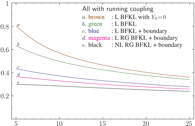
Figure 7: The logarithmic derivative of the saturation momentum $\lambda_{s}$ as a function of the rapidity $Y$ for running coupling.

Even though one cannot have such nice analytic expressions when considering the improved kernels, the results are not so hard to obtain since they involve the numerical solution of algebraic transcendental equations [89]. We summarize all cases in the plots in Fig. 7. In order to understand properly all the results, we have also plotted the first three lines which correspond to the analytic expression given in Eq. (35). Line-a is the first term with $Y_{0}=0$ while Line-b corresponds to the same term but with a typical value for $Y_{0}$ which is of order $\mathcal{O}(1)$. Line-c stands for the full expression in (35). Line-d and Line-e represent the improved kernels at leading and next to leading order respectively. Notice that all the lines will “merge” together at very high values of rapidity, since the leading term will become more and more dominant over the corrections as the coupling decreases along $Q_{s}$. The NLO result is stable in the sense that it adds a small correction to the leading one. We should mention that the NLO result is practically constant, $\lambda_{s}\simeq 0.3$ in the region $Y=5-10$. This is in good agreement with the phenomenology [57, 58, 59, 60]. However, it is not clear whether this theoretical value should be trusted or not. As we shall see in the forthcoming sections, the JIMWLK equation misses important contributions, which result in corrections that are much more significant than any NLO BFKL correction.

7 Deficiencies of the Balitsky-JIMWLK Hierarchy

Even though the Balitsky-JIMWLK hierarchy encompasses nicely the BFKL evolution and the merging of Pomerons at finite-$N_{c}$, it faces certain crucial problems. These problems, which we will immediately discuss, are related to each other, and therefore it seems that some unique element is missing from the CGC effective theory in the form it has been developed so far.

(i) The first problem is the extreme sensitivity of the JIMWLK equation to the ultraviolet. Since in the high momentum region the non-linearities are unimportant, we understand that this issue can be analyzed within the BFKL evolution. Let us try to reconstruct the solution in two (or more) global steps by completeness. To be more precise, let us first assume that we find the solution $T(Q,Y)$ by evolving the system from zero rapidity to rapidity $Y$. Now let us imagine that we evolve from zero to, say, $Y/2$. Then we can consider the solution $T(Q,Y/2)$ as the initial distribution and subsequently evolve to $Y$ to obtain $T(Q,Y)$. As we show in Appendix H, the solution obtained from this procedure will coincide with the one obtained from the single global evolution step, so long as we include (at least) the contributions from all momenta such that $\ln(Q^{2}/Q_{s}^{2})\lesssim\sqrt{D_{s}Y/2}$, in the initial condition at $Y/2$. Of course there is no reason to cut the momenta that lie outside the diffusion radius, but this algorithm reveals the width of the momentum phase space which is important for a self-consistent solution. This feature brings us in a quite embarrassing situation; as $Y$ increases, this phase space will open up more and more to momenta above the saturation line, and moreover the big numerical value of the coefficient $D_{s}$ will make the problem even worse. For instance, when one finds the saturation momentum to be a few GeV, at the same time one is sensitive to momenta a few orders of magnitudes above. Notice, that this explains why in the numerical solutions of both the BK [76, 101, 102, 64, 103, 104] and the JIMWLK equation [93], one had to go very far to the ultraviolet in order to obtain a reasonably accurate solution. In the running coupling case the situation is somewhat better, since the coupling decreases at higher momenta, and thus the effects of these seemingly non-physical contributions are reduced. Indeed, as we saw in Sec. 6, the “diffusion” radius increases much slower, namely $R_{D}\sim Y^{1/6}$. Nevertheless, the theoretical problem still exists.

(ii) Quite surprisingly, the second problem is the violation of unitarity. Here we shall not analyze the argument in detail [34], but only indicate its essence. Assume that we want to calculate the amplitude close to, but above, the saturation line in the two ways we described in the previous paragraph. Then one will have

$$1>c=T\sim\frac{1}{\alpha_{s}^{2}}\,T_{1}\,T_{2},$$ (37)

where $T_{1}$ and $T_{2}$ denote the contributions of the two successive steps. It is clear that for $T_{1}<\alpha_{s}^{2}$ the above equation imposes that the second step satisfy $T_{2}>1$. Thus, all the paths which go through the region to the right of the fluctuation line (the terminology will be understood in a while) in Fig. 6 will violate unitarity in the intermediate steps of the evolution. Returning to the problem we discussed in (i), and noticing that the diffusion radius extends to the region where the amplitude can be much smaller than $\alpha_{s}^{2}$, we see that these contributions from the ultraviolet region must be indeed non-physical.

These unitarity violating paths were “discovered” when dipole-dipole scattering was studied in the presence of saturation with the additional, but clearly natural, condition that the amplitude be Lorentz invariant [34], even though at that time it was not realized that they are part of JIMWLK evolution. A calculation of the saturation momentum was performed by cutting these paths with an absorptive UV boundary (in addition to the IR one), and the corrections found were huge. In Sec. 15 we shall review/obtain this result in a very simple way. We should say here, that in [35] a spectacular analogy with the physics and the results of the stochastic FKPP (sFKPP) equation was observed, and the significance of fluctuation effects in the low density region $T\sim\alpha_{s}^{2}\Leftrightarrow\varphi\sim\alpha_{s}$ was understood. Still, the fact that one needs to go beyond the JIMWLK equation was not yet realized.

(iii) The third problem in the evolution equations we have discussed so far, is the absence of Pomeron splittings [38]. As we have seen, the mechanism of Pomeron mergings, which was essential to describe properly the physics near the unitarity limit, is described by the JIMWLK equation. If we expand the Hamiltonian in powers of $g$, then each term will involve at least two factors of the color field $\alpha$ and exactly two functional derivatives with respect to $\alpha$. Then a typical term in the evolution equation of the $n$-th point correlator of the color fields will have the structure (suppressing the coordinates’ dependence, which is not important for the forthcoming argument)

$$\frac{\partial\langle\alpha^{n}\rangle}{\partial Y}=\langle H\,\alpha^{n}\rangle\sim\bigg{\langle}\underbrace{\alpha\,\alpha...\alpha}_{\geq 2}\frac{\delta}{\delta\alpha}\,\frac{\delta}{\delta\alpha}\,\alpha^{n}\bigg{\rangle}\sim\langle\alpha^{m}\rangle\quad{\rm with}\quad m\geq n.$$ (38)

So, as we already knew, the JIMWLK Hamiltonian can describe BFKL dynamics and Pomeron mergings. But the natural question at this point is, “how could we have two or more ladders in the first place?” Clearly JIMWLK cannot do that, since one would need $m<n$ in Eq. (38). One option would be to consider a large nucleus target, which contains many valence quarks and antiquarks. These sources can evolve with rapidity and produce many BFKL Pomerons, which will merge when saturation becomes important. However, this is just a special case because of its particular initial condition, and the dynamical problem is not solved. Furthermore, even in the nucleus, there will always be some dilute “tail” corresponding to the high momentum modes. After some evolution, and since the saturation momentum increases, these modes will need to saturate. But still there is no dynamics to produce the corresponding Pomerons which will eventually merge. Thus, the only solution to this problem is to find how QCD will give rise to the Pomeron splittings. Then indeed, one could start, for example, even from a single bare dipole, and end up with a fully saturated wavefunction. As we shall see in the following sections, when “completing” the theory by including the diagrams which were “forgotten” [38, 39], and which lead to the splittings of Pomerons, we will also automatically solve the two problems presented in (i) and (ii).

8 The Missing Diagrams

Since one of the basic problems of the JIMWLK equation is the absence of Pomeron Splittings, one should consider diagrams like the third one in Fig. 8 in order to resolve the issue. Indeed, this diagram corresponds to a transition from one to two Pomerons. If one wants to “measure” two Pomerons, and in the two-gluon exchange approximation, one needs to probe the hadron wave function with two projectile dipoles, and this is what is shown in the typical diagrams in Fig. 8. The first diagram corresponds to normal BFKL evolution, with the one of the Pomerons being a spectator. As indicated, it is of order $\bar{\alpha}_{s}\Delta Y\mathcal{O}(\alpha_{s}^{2}\varphi^{2})$; $\bar{\alpha}_{s}\Delta Y$ for the evolution step, $\alpha_{s}^{2}$ for the four fermion-gluon vertices and $\varphi^{2}$ since there were two Pomerons before the step. Similarly the second diagram, which corresponds to a $2\to 1$ Pomeron transition, with the third Pomeron being a spectator, is of order $\bar{\alpha}_{s}\Delta Y\mathcal{O}(\alpha_{s}^{3}\varphi^{3})$. Both diagrams are described by the JIMWLK equation. The third diagram is of order $\bar{\alpha}_{s}\Delta Y\mathcal{O}(\alpha_{s}^{3}\varphi)$, since there are six vertices and one Pomeron before the step. Clearly this diagram is suppressed with respect to at least one of the first two diagrams when $\varphi\gg\alpha_{s}$, and this is the reason why it was neglected in the derivation of the JIMWLK equation, which aimed to describe a high density system. However, due to the non-locality of the evolution kernel which leads to the ultraviolet diffusion, this diagram will give significant contributions through the intermediate evolution steps. It is rather crucial to notice that this diagram becomes important when $\varphi\sim\alpha_{s}$ or equivalently when $T\sim\alpha_{s}^{2}$, which corresponds precisely to the line at which JIMWLK faces its unitarity problem. This is the fluctuation line we have already shown in Fig. 6, and which divides the region of normal BFKL evolution from the low density region. The latter is characterized by fluctuations and this explains in a way why we need (at least) two projectiles dipoles.

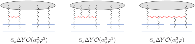
Figure 8: Diagrams contributing to the evolution of two BFKL Pomerons. The third diagram was “missed” in JIMWLK.

By probing with one dipole we will measure only the “one-point” function, say the gluon occupation number. But this will not release any information about the two-point function, since in a dilute system the pair density is affected by the fluctuations and is not simply the square of the single density. Thus one needs to probe with two dipoles in order to measure the non-trivial low density correlations. This analysis also implies that, presumably, the first Balitsky equation will not change. But of course, any mean field approximation to this equation will not be valid any more, since the presence of fluctuations will have a significant impact on its non-linear term. In the next section we shall shortly describe some elementary but essential, for our purposes, features of the color dipole picture. We shall return to give a more quantitative analysis of what we discussed here, in Sec. 10.

9 Evolution of Dipoles

Since we have realized that what we need to correct in the JIMWLK equation is its low-density limit, let us look more carefully at the non-saturated part of the wavefunction of a hadron. We will first consider the large-$N_{c}$ limit case, that is, the hadron is supposed to be composed of color dipoles. When the dipole density is not too high, i.e when $n\ll 1/\alpha_{s}^{2}$, the emission of a soft gluon from a dipole will not be affected by the remaining surrounding dipoles. We have already written the (positive and well-defined) probability for this emission in Eq. (2) with the derivation given in Appendix A. From now on we shall not present the original formulation of this dipole picture [5, 6, 7, 8], rather we will follow the procedure developed in [105] which is better suited to our purposes.

One can write a master equation describing the evolution of the probabilities to find a given configuration. To be more specific, a given configuration is characterized by the number of dipoles $N$ and by $N-1$ transverse coordinates $\{\bm{z}_{\imath}\}=\{\bm{z}_{1},\bm{z}_{2},\dots,\bm{z}_{N-1}\}$, such that the coordinates of the $N$ dipoles are $(\bm{z}_{0},\bm{z}_{1})$, $(\bm{z}_{1},\bm{z}_{2})$,…,$(\bm{z}_{N-1},\bm{z}_{N})$, with $\bm{z}_{0}\equiv\bm{u}_{0}$ and $\bm{z}_{N}\equiv\bm{v}_{0}$, assuming that the initial state was a dipole $(\bm{u}_{0},\bm{v}_{0})$. The probability $P_{N}(\{\bm{z}_{\imath}\};Y)$ to find a given configuration at rapidity $Y$ obeys

$$\frac{\partial P_{N}(\bm{z}_{1},...,\bm{z}_{N-1};\!Y)}{\partial Y}= \!\!\!\!\!\!\frac{\bar{\alpha}_{s}}{2\pi}\!\sum_{\imath=1}^{N-1}\!\mathcal{M}(\bm{z}_{\imath-1},\bm{z}_{\imath+1},\bm{z}_{\imath})P_{N-1}(\bm{z}_{1},...,\not{\bm{z}}_{\imath},...,\bm{z}_{N-1};\!Y)$$ (39)

$$\!\!\!\!\!\!-\frac{\bar{\alpha}_{s}}{2\pi}\sum_{\imath=1}^{N}\int\limits_{\bm{z}}\mathcal{M}(\bm{z}_{\imath-1},\bm{z}_{\imath},\bm{z})\,P_{N}(\bm{z}_{1},...,\bm{z}_{N-1};\!Y),$$

where a slashed variable is omitted. The interpretation is quite obvious; while the gain (first) term describes the formation of an $N$-dipoles state through the splitting of a dipole in a pre-existing state with $N-1$ dipoles, the second term describes the emission of a soft gluon from the $N$-dipoles state, which leads to a state with $N+1$ dipoles and therefore to a loss of probability. It is straightforward to show that the total probability is conserved, which is one of the requirements that Eq. (39) be well-defined. The expectation value of an operator $\mathcal{O}$ which depends only on dipole coordinates is given by

$$\langle\mathcal{O}(Y)\rangle\,=\,\sum_{N=1}^{\infty}\int{\rm d}\Gamma_{N}\,P_{N}(\{\bm{z}_{\imath}\};Y)\,\mathcal{O}_{N}(\{\bm{z}_{\imath}\}),$$ (40)

where the phase space integration is simply ${\rm d}\Gamma_{N}\,=\,{\rm d}^{2}\bm{z}_{1}{\rm d}^{2}\bm{z}_{2}\dots\rm d^{2}\bm{z}_{N-1}$. Then by using the master equation (39) one can show that

$$\frac{\partial\langle\mathcal{O}(Y)\rangle}{\partial Y}=\frac{\bar{\alpha}_{s}}{2\pi}\sum_{N=1}^{\infty}\int \!\!\!\!\!\!{\rm d}\Gamma_{N}\,P_{N}(\{\bm{z}_{\imath}\};Y)\,\sum_{i=1}^{N}\int\limits_{\bm{z}}\,{\mathcal{M}}({\bm{z}}_{\imath-1},{\bm{z}}_{\imath},{\bm{z}})$$ (41)

$$\!\!\!\!\!\!\times\left[-{\mathcal{O}}_{N}(\{\bm{z}_{\imath}\})+{\mathcal{O}}_{N+1}(\{\bm{z}_{\imath},\bm{z}\})\,\right],$$

where the $\bm{z}$ argument in ${\mathcal{O}}_{N+1}$ is to be placed between $\bm{z}_{\imath-1}$ and $\bm{z}_{\imath}$. In what follows, we shall use Eq. (41) to derive evolution equations for the dipole number densities. Consider first the average number density of dipoles at $(\bm{u},\bm{v})$. The corresponding part for an $N$-dipole configuration is

$$n_{N}(\bm{u},\bm{v})=\sum_{\jmath=1}^{N}\delta(\bm{z}_{\jmath-1}-\bm{u})\delta(\bm{z}_{\jmath}-\bm{v}),$$ (42)

so that $\langle n_{\bm{u}\bm{v}}\rangle$ will be given by the r.h.s. of Eq. (40) if we let $O_{N}\to n_{N}$. Then by making use of Eq. (41) and after relatively simple manipulations one arrives at the evolution equation for the average of the dipole number density $\langle n_{\bm{u}\bm{v}}\rangle$ which reads

$$\frac{\partial\langle n_{\bm{u}\bm{v}}\rangle}{\partial Y} \!\!\!\!\!\!=\frac{\bar{\alpha}_{s}}{2\pi}\int\limits_{\bm{z}}\left[{\mathcal{M}}_{{\bm{u}}{\bm{z}}{\bm{v}}}\langle n_{\bm{u}\bm{z}}\rangle+{\mathcal{M}}_{{\bm{z}}{\bm{v}}{\bm{u}}}\langle n_{\bm{z}\bm{v}}\rangle-{\mathcal{M}}_{{\bm{u}}{\bm{v}}{\bm{z}}}\langle n_{\bm{u}\bm{v}}\rangle\right]$$ (43)

$$\!\!\!\!\!\!\equiv\frac{\bar{\alpha}_{s}}{2\pi}\int\limits_{\bm{z}}\mathcal{K}_{\bm{u}\bm{v}\bm{z}}\otimes\langle n_{\bm{u}\bm{v}}\rangle.$$

This is simply the BFKL equation for the dipole density, and its pictorial representation is given in Fig. 9. This equation should be read in the “passive” point of view, in contrast to Eq. (3). That is, as it was obvious in the derivation, the r.h.s. contains what was existing before the evolution step. The first term is proportional to the probability for a dipole $(\bm{u},\bm{z})$ to split into two new dipoles $(\bm{u},\bm{v})$ and $(\bm{v},\bm{z})$ times the initial density at $(\bm{u},\bm{z})$. Since we want to find the change in the density at $(\bm{u},\bm{v})$ only the first of these two child dipoles is measured. Similarly for the second term. The last term is proportional to the probability for a dipole $(\bm{u},\bm{v})$ to split into two new dipoles times the initial density at $(\bm{u},\bm{v})$ and naturally gives a negative contribution. Notice that the loss term in Eq. (39) was crucial in order to obtain this virtual contribution.

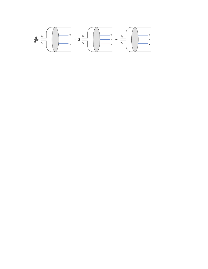
Figure 9: Evolution of the dipole density for a dilute hadron at large $N_{c}$.

As we show in Appendix C, this equation leads to the BFKL equation, Eq. (3), for the scattering amplitude of a projectile dipole off the dilute hadron, when we assume the two gluon exchange approximation which is appropriate in this dilute limit.

Now we can follow the same procedure to derive the analogous equation for the dipole pair density [38]. The corresponding part for a given $N$-dipole configuration is

$$n_{N}^{(2)}(\bm{u}_{1}\bm{v}_{1};\bm{u}_{2},\bm{v}_{2})=\!\sum_{\begin{subarray}{c}\jmath,k=1\\ \jmath\neq k\end{subarray}}^{N}\!\delta(\bm{z}_{\jmath-1}\!-\!\bm{u}_{1})\delta(\bm{z}_{\jmath}\!-\!\bm{v}_{1})\delta(\bm{z}_{k-1}\!-\!\bm{u}_{2})\delta(\bm{z}_{k}\!-\!\bm{v}_{2}),$$ (44)

and following the same procedure as in the case of the dipole density, we arrive at the evolution equation

$$\frac{\partial\langle n^{(2)}_{\bm{u}_{1}\bm{v}_{1};\bm{u}_{2}\bm{v}_{2}}\rangle}{\partial Y}=\frac{\bar{\alpha}_{s}}{2\pi}\,\bigg{[} \!\!\!\!\!\!\int_{\bm{z}}\mathcal{K}_{\bm{u}_{1}\bm{v}_{1}\bm{z}}\otimes\langle n^{(2)}_{\bm{u}_{1}\bm{v}_{1};\bm{u}_{2}\bm{v}_{2}}\rangle$$ (45)

$$\!\!\!\!\!\!+\,\delta_{\bm{u}_{2}\bm{v}_{1}}\mathcal{M}_{\bm{u}_{1}\bm{v}_{2}\bm{u}_{2}}\langle n_{\bm{u}_{1}\bm{v}_{2}}\rangle\bigg{]}\,+\,1\leftrightarrow 2.$$

with the notation introduced in Eq. (43). The two terms on the r.h.s. correspond to the two typical contributing diagrams in Fig. 10. The first term (which in turn is a sum of three terms) corresponds to the BFKL evolution of the first dipole while the second dipole remains a spectator. The second term corresponds to a single dipole initial density and the mother dipole splits into two new dipoles both of which are “measured”. We shall refer to this term as the “splitting” term, and this in the sense that a lower moment of the density gives rise to a higher moment of the density.

Of course one can continue and write the evolution equation for the $\kappa$-th density [106]. We shall not do it here, since it is just a matter of proper combinatorics. It is clear that there will be $\kappa$ terms corresponding to normal BFKL evolution where only one dipole is evolving and $\kappa\!-\!1$ are spectators. Furthermore, there will be $\kappa(\kappa-1)$ splitting terms, according to the terminology we just defined, which will be proportional to the $\kappa\!-\!1$-th density where the $\kappa\!-\!2$ dipoles will be spectators.

Figure 10: Evolution of the dipole pair density for a dilute hadron at large $N_{c}$. The loss term of the normal BFKL evolution is not shown.

These splitting contributions, or to be more precise their analogue, were not included in the JIMWLK equation. We already start to see the consequences, since it is trivial to show that the hierarchy of equations obeyed by the density moments is not consistent with any sort of factorization, for example

$$\langle n^{(2)}_{\bm{u}_{1}\bm{v}_{1};\bm{u}_{2}\bm{v}_{2}}\rangle\neq c\langle n_{\bm{u}_{1}\bm{v}_{1}}\rangle\langle n_{\bm{u}_{2}\bm{v}_{2}}\rangle.$$ (46)

This factorization is “broken” because of the splittings terms which become important in the region $n\sim 1$ (or equivalently when $T\sim\alpha_{s}^{2}$), that is, when fluctuations in the number density of particles become a significant effect. We need to say here that in the original formulation of the dipole picture the equation for the dipole-pair density (and the higher moments) was not written as given in Eq. (45), but in an equivalent form in which the fluctuations were more difficult to recognize. Nevertheless, based on that picture, these low-density fluctuations and some of their consequences were in fact “seen” in the numerical simulations of the wavefunction of an evolved dipole and of the approach to unitarity [36, 37].

10 Splittings of Pomerons, Large-$N_{c}$ Equations and the Langevin Equation

Now that we have derived the equation for the dipole-pair density, it is not hard to transform to the corresponding equation for the amplitude of two given external dipoles to scatter off the target. To the order of accuracy it is enough to consider that dipoles scatter in the two-gluon exchange approximation. This elementary scattering amplitude for two dipoles $(\bm{x},\bm{y})$ and $(\bm{u},\bm{v})$ is calculated in Appendix B and it reads (see e.g. [107, 108])

$$T_{0}(\bm{x}\bm{y}|\bm{u}\bm{v})= \!\!\!\!\!\!\frac{\alpha_{s}^{2}}{8}\,\frac{N_{c}^{2}-1}{N_{c}^{2}}\,\ln^{2}\left[\frac{(\bm{x}-\bm{v})^{2}(\bm{y}-\bm{u})^{2}}{(\bm{x}-\bm{u})^{2}(\bm{y}-\bm{v})^{2}}\right]$$

$$\equiv \!\!\!\!\!\!\,\alpha_{s}^{2}\,\frac{N_{c}^{2}-1}{N_{c}^{2}}\,\mathcal{A}_{0}(\bm{x}\bm{y}|\bm{u}\bm{v}).$$ (47)

For what follows, we shall set the fraction involving the color factor equal to one, since we have already assumed the large-$N_{c}$ limit in our analysis. To this end, the amplitude for the projectile dipole $(\bm{x},\bm{y})$ to scatter off the target will be

$$\langle T_{\bm{x}\bm{y}}\rangle=\alpha_{s}^{2}\int\limits_{\bm{u}\bm{v}}\mathcal{A}_{0}(\bm{x}\bm{y}|\bm{u}\bm{v})\,\langle n_{\bm{u}\bm{v}}\rangle\Rightarrow\langle n_{\bm{u}\bm{v}}\rangle+\langle n_{\bm{v}\bm{u}}\rangle=\frac{4}{g^{4}}\,\nabla_{\bm{u}}^{2}\nabla_{\bm{v}}^{2}\langle T_{\bm{u}\bm{v}}\rangle,$$ (48)

where in the second part, valid for $\bm{u}\neq\bm{v}$, we have inverted the equation to obtain the symmetrized dipole density in terms of the amplitude for our later convenience. Now let us consider the scattering of a pair of dipoles $(\bm{x}_{1},\bm{y}_{1})$ and $(\bm{x}_{2},\bm{y}_{2})$ off the target. Then the extension of Eq. (48) reads

$$\langle T_{\bm{x}_{1}\bm{y}_{1}}T_{\bm{x}_{2}\bm{y}_{2}}\rangle=\alpha_{s}^{4}\int\limits_{\bm{u}_{\imath}\bm{v}_{\imath}}\mathcal{A}_{0}(\bm{x}_{1}\bm{y}_{1}|\bm{u}_{1}\bm{v}_{1})\,\mathcal{A}_{0}(\bm{x}_{2}\bm{y}_{2}|\bm{u}_{2}\bm{v}_{2})\,\langle n^{(2)}_{\bm{u}_{1}\bm{v}_{1};\bm{u}_{2}\bm{v}_{2}}\rangle.$$ (49)

Clearly, in writing the above equation, we have assumed that two dipoles do not interact with the same dipole. We need to say that neither a large-$N_{c}$ nor a small coupling argument justifies this assumption. Nevertheless, such processes will be suppressed at higher energies, as they will grow like a single BFKL Pomeron. Now by differentiating Eq. (49) and using the last, linear in $\langle n\rangle$, term in Eq. (45) for the evolution of the dipole pair density (the bilinear terms give rise to the normal BFKL evolution of $\langle TT\rangle$, which we already know how to write), we obtain the splitting contribution to the evolution of the dipole-pair amplitude, which reads [38, 39, 40, 43] (see also [109, 110])

$$\frac{\partial\langle T_{\bm{x}_{1}\bm{y}_{1}}T_{\bm{x}_{2}\bm{y}_{2}}\rangle}{\partial Y}\,\bigg{|}_{\rm split}=\left(\frac{\alpha_{s}}{2\pi}\right)^{2}\frac{\bar{\alpha}_{s}}{2\pi}\!\int\limits_{\bm{u}\bm{v}\bm{z}} \!\!\!\!\!\!\mathcal{M}_{\bm{u}\bm{v}\bm{z}}\,\mathcal{A}_{0}(\bm{x}_{1}\bm{y}_{1}|\bm{u}\bm{z})\,\mathcal{A}_{0}(\bm{x}_{2}\bm{y}_{2}|\bm{z}\bm{v})\,$$ (50)

$$\!\!\!\!\!\!\times\nabla_{\bm{u}}^{2}\nabla_{\bm{v}}^{2}\,\langle T_{\bm{u}\bm{v}}\rangle.$$

Notice that the poles of the kernel cancel with the zeros of the dipole-dipole scattering amplitude. The pictorial interpretation of this equation is given in Fig. 11. A dipole $(\bm{u},\bm{v})$ of the target splits into two new dipoles $(\bm{u},\bm{z})$ and $(\bm{z},\bm{v})$, leading to the dipole kernel in Eq. (50). The two daughter dipoles scatter with the two projectile dipoles, as represented by the two $\mathcal{A}_{0}$’s in the equation. Finally the last term is proportional to the initial dipole density, which has been expressed in terms of the single scattering amplitude by making use of Eq. (48).

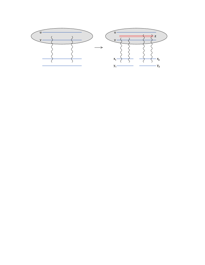
Figure 11: Splitting contribution to the dipole pair scattering.

This is the term that we would like to add to the r.h.s. of the second (large-$N_{c}$) Balitsky equation. It corresponds to the splitting of one Pomeron into two, and this is really the mechanism for the generation of correlations in higher-point functions which have important consequences to the subsequent evolution of the system. For example, through Eq. (50) the single scattering amplitude will give rise to correlations in the dipole-pair scattering amplitude and their significance will be realized when they feedback to the single amplitude through the first Balitsky equation.

It is trivial to add the corresponding splitting term in the $\kappa$-th equation of the large-$N_{c}$ Balitsky hierarchy. In the r.h.s. of the evolution equation for the amplitude for $\kappa$ dipoles there will be $\kappa(\kappa\!-\!1)/2$ terms proportional to the amplitude for $\kappa\!-\!1$ dipoles, and where in each term $\kappa\!-\!2$ dipoles will be simply spectators. Therefore, the new hierarchy can be easily inferred from Eqs. (3), (12) and (50), since in the $\kappa$-th evolution equation the relevant processes are $1\to 1$, $1\to 2$ and $2\to 1$ Pomeron transitions, with all other Pomerons being just spectators, and one just needs to take into account all the possible permutations. Thus, it is not necessary to present the full set of equations here (we shall give an equivalent compact form in Eq. (52) below), rather we shall indicate only its structure by suppressing the transverse coordinates. It reads

$$\frac{\partial\langle T^{\kappa}\rangle}{\partial Y}=\kappa\,\bar{\alpha}_{s}\,\langle T^{\kappa}\rangle-\kappa\,\bar{\alpha}_{s}\,\langle T^{\kappa+1}\rangle+\frac{\kappa(\kappa-1)}{2}\,\bar{\alpha}_{s}\,\alpha_{s}^{2}\,\langle T^{\kappa\!-\!1}\rangle,$$ (51)

where the $\kappa$-dependent coefficients stand for the number of terms arising from the permutations.

For the reasons analyzed in Sec. 9, it is clear that our hierarchy is not consistent with any sort of factorizing solution; the low density behavior of the theory has totally changed with respect to the theory without Pomeron splittings. Therefore, one has to find alternative ways to deal with this set of equations. One way to do that, is to reformulate the problem as a single stochastic equation. Indeed, the Langevin equation

$$\!\!\!\!\!\frac{1}{\bar{\alpha}_{s}}\frac{\partial T_{\bm{x}\bm{y}}}{\partial Y} \!\!\!\!\!\!=\frac{1}{2\pi}\int\limits_{\bm{z}}\mathcal{M}_{\bm{x}\bm{y}\bm{z}}\,[T_{\bm{x}\bm{z}}+T_{\bm{z}\bm{y}}-T_{\bm{x}\bm{y}}-T_{\bm{x}\bm{z}}T_{\bm{z}\bm{y}}]$$ (52)

$$\!\!\!\!\!\!+\,\frac{\alpha_{s}}{2\pi}\,\sqrt{\frac{1}{2\pi}}\!\int\limits_{\bm{u}\bm{v}\bm{z}}\!\mathcal{A}_{0}(\bm{x}\bm{y}|\bm{u}\bm{z})\,\frac{|\bm{u}-\bm{v}|}{(\bm{u}-\bm{z})^{2}}\,\sqrt{\nabla_{\bm{u}}^{2}\nabla_{\bm{v}}^{2}T_{\bm{u}\bm{v}}}\,\,\nu(\bm{u}\bm{v}\bm{z};Y),$$

where the noise satisfies

$$\langle\nu(\bm{u}_{1}\bm{v}_{1}\bm{z}_{1};Y)\nu(\bm{u}_{2}\bm{v}_{2}\bm{z}_{2};Y^{\prime})\rangle=\delta_{\bm{u}_{1}\bm{v}_{2}}\delta_{\bm{v}_{1}\bm{u}_{2}}\delta_{\bm{z}_{1}\bm{z}_{2}}\delta(\bar{\alpha}_{s}Y\!-\!\bar{\alpha}_{s}Y^{\prime}),$$ (53)

and where all other noise correlators vanish, gives an equivalent description [39]. We show this equivalence in Appendix I for a simple zero-dimensional model, while the generalization to the QCD problem at hand is straightforward. However, because of the complexity of the noise correlation, this form may not be the best option in the search for numerical solutions. Nevertheless, one can rely on certain approximations to gain a first idea on the new features of the evolution. Assuming that the elementary dipole-dipole scattering amplitude is local in transverse coordinates, performing a coarse-graining in impact parameter space and defining the Bessel transformation $\varphi$ of the scattering amplitude one arrives at [38]

$$\frac{1}{\bar{\alpha}_{s}}\frac{\partial\varphi(\bm{k})}{\partial Y}= \!\!\!\!\!\!\frac{1}{2\pi}\int\limits_{\bm{p}}\frac{\bm{k}^{2}}{\bm{p}^{2}(\bm{k}-\bm{p})^{2}}\left[2\,\frac{\bm{p}^{2}}{\bm{k}^{2}}\,\varphi(\bm{p})-\varphi(\bm{k})\right]-\varphi^{2}(\bm{k})$$ (54)

$$\!\!\!\!\!\!+\sqrt{2\,c\,\alpha_{s}^{2}\,\varphi(\bm{k})}\,\,\nu(\bm{k,Y}),$$

with $\nu(\bm{k},Y)$ a Gaussian white noise, i.e. the only non-vanishing correlator is $\langle\nu(\bm{k}_{1},Y)\,\nu(\bm{k}_{2},Y^{\prime})\rangle=\delta(\bar{\alpha}_{s}Y-\bar{\alpha}_{s}Y^{\prime})\,\delta(\bm{k}_{1}^{2}-\bm{k}_{2}^{2})\,\bm{k}_{1}^{2}$, and where $c$ is a constant of order $\mathcal{O}(1)$. Notice that, up to an overall normalization factor of order $\mathcal{O}(1/\bar{\alpha}_{s})$, $\varphi(\bm{k})$ is the unintegrated gluon distribution. A numerical solution to this equation has been given in [112]. Furthermore, if one performs a saddle point approximation to the BFKL kernel in Eq. (54), the resulting equation is the stochastic FKPP equation which has been studied numerically in [113]. So long as the energy dependence of $Q_{s}$ is concerned, the results from these numerics are consistent with the ones from the analytical approach that we will present in Sec. 15.

It is appropriate to make here a few important comments on the hierarchy we have derived, and which is compactly written in the “exact” Langevin Eq. (52). The first is with respect to the strength of each term. In the low density region where $T\sim\alpha_{s}^{2}$, one can see in the Langevin equation that both the noise (splitting) term and the BFKL terms are of the same order, while the merging term is suppressed by a factor $\mathcal{O}(\alpha_{s}^{2})$. In the intermediate region where $\alpha_{s}^{2}\ll T\ll 1$, the BFKL terms dominate, and in the region near the unitarity limit $T\sim 1$, the BFKL terms and the merging term are of the same order, while the noise term is subdominant by a factor $\mathcal{O}(\alpha_{s}^{2})$. The second comment we should make is that, as in the case of the Balitsky equations, $T=1$ is still a fixed point of the evolution; the noise term in the Langevin equation vanishes for constant $T$ due to the presence of the Laplacians. We should also say that we do not expect the term we added to describe properly the Pomeron splittings in the high density region, since we have heavily relied on the two-gluon exchange approximation. In fact, even though we expect on general grounds the Pomeron splittings to be positive, the term we added can be negative in some regions [115]. Nevertheless, this is not very worrisome, since Pomeron splittings are supposed to dominate in the low density region, and to this end the leading contribution has been taken into account. In that region the r.h.s. of Eq. (50) is clearly positive, since $\nabla_{\bm{u}}^{2}\nabla_{\bm{v}}^{2}T_{\bm{u}\bm{v}}$ is in fact proportional to the dipole density which is positive, while away from that region the term is anyway suppressed with respect to the other contributions as we have just seen.

Before closing this section, and in order to cross-check that our approach was correct, let us compare with a well-known result obtained from the construction of Pomeron vertices in perturbative QCD. By neglecting the non-linear evolution terms, it is clear that one arrives at a solvable problem. Thus, by first solving the BFKL equation, and subsequently solving the second equation in the hierarchy, which is an inhomogeneous one, and assuming the initial condition $\langle TT\rangle=0$, we find [39]

$$\langle T_{\bm{x}_{1}\bm{y}_{1}}T_{\bm{x}_{2}\bm{y}_{2}}\rangle=\left(\frac{\alpha_{s}}{2\pi}\right)^{2}\frac{\bar{\alpha}_{s}}{2\pi}\,\int\limits_{0}^{Y}{\rm d}y\int\limits_{\bm{u}\bm{v}\bm{z}} \!\!\!\!\!\!\mathcal{M}_{\bm{u}\bm{v}\bm{z}}\,\mathcal{A}_{Y-y}(\bm{x}_{1}\bm{y}_{1}|\bm{u}\bm{z})\,\mathcal{A}_{Y-y}(\bm{x}_{2}\bm{y}_{2}|\bm{z}\bm{v})\,$$ (55)

$$\!\!\!\!\!\!\times\nabla_{\bm{u}}^{2}\nabla_{\bm{v}}^{2}\langle T_{\bm{u}\bm{v}}\rangle.$$

This coincides with the large-$N_{c}$ triple Pomeron vertex as given in [31].

11 Loops of Pomerons

Since the hierarchy presented in the previous section contains both splittings and mergings of Pomerons, it is clear that Pomeron loops will be generated in the course of evolution. For example, let us find the minimal loop, which will be formed after a two step evolution. This is depicted in the middle diagram of Fig. 12. In the first step the dipole emits a soft gluon which, as always, can be considered as a quark-antiquark pair and the two daughter dipoles “radiate” two “elementary” Pomerons. In the second step, the two Pomerons merge into one through the emission of another soft gluon.

Of course one understands that a “real” Pomeron loop will be formed after a large number of steps, if we dress all parts of the process with normal BFKL evolution. Following this procedure we can construct the Pomeron loop vertex and let us make a short digression here, to say that one can do the same for all kinds of such Pomeron vertices (i.e. vertices integrated over a large rapidity interval) that one can imagine, e.g. for the triple Pomeron vertex given at the end of the previous section. Of course this is a very tedious procedure, and at the end one has to embed all possible allowed combinations of these vertices into a huge diagram, which has the two initial colliding objects at its two ends. Furthermore, given the non-linearities of the system, it is not clear whether this approach to the problem can be successful or not. Therefore it seems that, instead of trying to calculate building blocks of the theory, it is more advantageous to deal with the full theory as a whole, i.e. the hierarchy of equations we just presented, or its generalization to finite-$N_{c}$ (when the latter becomes available). Of course, in order to construct the evolution equations it is necessary to know the “reggeized” gluon transition vertices (i.e. the vertices for a single step in rapidity) [9, 30]. In the large-$N_{c}$ limit, and for the specific observables that we were interested in, we only needed to have the $2\to 4$ vertex in coordinate space which is simply the dipole kernel $\mathcal{M}_{\bm{x}\bm{y}\bm{z}}$.

Let us now return to the calculation of the minimal Pomeron loop, since the result will reveal some very interesting features. In terms of the evolution equations, and starting from the single scattering amplitude $\langle T\rangle$, the diagram in Fig. 12 corresponds to the generation of $\langle TT\rangle$ through the fluctuation (splitting) term given in Eq. (50), which subsequently gives feedback to $\langle T\rangle$ through the non-linear term of the first Balitsky equation. Assuming that the initial state of the target was described by a single dipole at $(\bm{u},\bm{v})$ and the projectile dipole is at $(\bm{x},\bm{y})$, it is easy to show that [43]

$$\mathbb{PL}^{0}=-2\,\alpha_{s}^{4}\left(\frac{\bar{\alpha}_{s}}{2\pi}\right)^{2}\int\limits_{\bm{z}\bm{w}}\mathcal{M}_{\bm{x}\bm{y}\bm{z}}\,\mathcal{M}_{\bm{u}\bm{v}\bm{w}}\,\mathcal{A}_{0}(\bm{x}\bm{z}|\bm{u}\bm{w})\,\mathcal{A}_{0}(\bm{z}\bm{y}|\bm{w}\bm{v})$$ (56)

times a factor of order $(\Delta Y)^{2}=({\rm step})^{2}$ which we have suppressed. We immediately see that this result is free of any possible divergencies, since the poles of the dipole kernels are canceled by the zeros of the $\mathcal{A}_{0}$’s. Furthermore, and as expected, the contribution of the Pomeron loop is negative and leads to a decrease of the scattering amplitude(s) in the course of evolution.

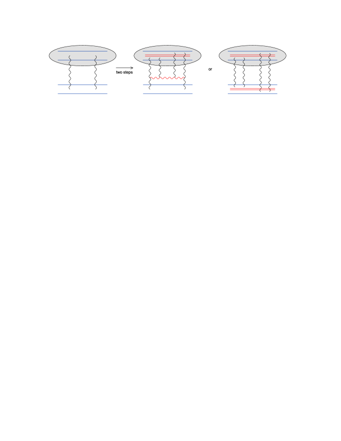
Figure 12: Formation of a loop under a two step evolution.

Even though we were thinking that we put the “whole” evolution in the wavefunction of the target dipole $(\bm{u},\bm{v})$, it is clear that Eq. (56) serves for an alternative interpretation, as shown in the last diagram in Fig. 12. Both the original, target and projectile, dipoles split into two child dipoles (each of them), processes which are represented by the two dipole kernels times $\bar{\alpha}_{s}^{2}$. Afterwards, the ensuing dipoles scatter with each other at the two-gluon exchange level, and this gives rise to the two $\mathcal{A}_{0}$’s accompanied by a factor $\alpha_{s}^{4}$. Therefore one arrives at the conclusion, that a merging of Pomerons in one of the scattering objects (here the target) can be equivalently considered as a splitting of Pomerons in the other object (here the projectile). Of course, one should keep in mind that whichever is the way we want to view the process, the soft gluon (the red horizontal gluon in the figures) is always emitted in the wavefunction of one of the two objects. This feature of exchanging splittings with mergings by jumping from the one wavefunction to the other, was already valid at the level of the Balitsky-JIMWLK evolution, where the mergings à la JIMWLK could be viewed as splittings à la Balitsky. But Eq. (56) contains more than that, since it allows for both type of processes inside the same wavefunction. Putting all these properties together, we shall see in the next section that we can formulate a precise duality condition, which is satisfied by the Hamiltonian governing the evolution of the hadronic system.

12 COM Frame, Duality and a Pomeron Effective Theory

Now we will discuss a remarkable duality property which is presumably satisfied by the complete Hamiltonian at high energy and at the leading logarithmic level. Here we shall describe the simplified case where the two colliding hadrons are described by non-saturated wavefunctions [43], while an approach to the general proof has been given in [42], where the idea of the duality was explicitly written for the first time.

So let us consider the scattering of two evolved dipoles. Assuming that the right (R) moving object is evolved by $Y-y$ and the left (L) moving one by $y$, one can write the average $S$-matrix as [105]

$$\langle S\rangle=\int\mathcal{D}\alpha_{\rm R}\,\mathcal{D}\alpha_{\rm L}\,Z_{Y\!-y}[\alpha_{\rm R}]\,Z_{y}[\alpha_{\rm L}]\,\exp\left[{\rm i}\int\limits_{\bm{z}}\rho^{a}_{\rm L}(\bm{z})\,\alpha^{a}_{\rm R}(\bm{z})\right].$$ (57)

The last exponential factor stands for the $S$-matrix for a given state of both the R and L evolved dipoles, and it is just the eikonal coupling between the color charge in the L object and the field created by the R object. Notice that it can be brought into a symmetric form under the exchange R$\leftrightarrow$L, by using the Poisson equation $\nabla_{\bm{z}}^{2}\alpha^{a}_{\rm R/L}(\bm{z})=-\rho^{a}_{\rm R/L}(\bm{z})$ and integrating by parts. To obtain the average $S$-matrix we simply integrate over all possible configurations for both wavefunctions. This formula would be exact in QED, however it has a restricted range of validity in QCD. As we have seen in QCD, and if one wants to include all multiple scattering contributions, one needs to use path order exponentials to account for the color matrices non-commutativity in the interaction vertices, so Eq. (57) cannot be correct in general. Nevertheless, it contains the possibility that any number of projectile dipoles interact with the same number of target dipoles, even though each individual dipole interacts, at most, only once. This simultaneous scattering of many dipoles is equivalent to a “multiple Pomeron exchange” and one expects the final result to respect unitarity limits. Thus, Eq. (57) goes much beyond the BFKL equation. We can show that all the above approximations and conclusions are meaningful in a frame which is not fully asymmetric, i.e. when $y=\kappa Y$, with $\kappa$ a constant of order $\mathcal{O}(1)$, but of course smaller than one, for example in the center of mass (COM) frame $y=Y/2$. Requiring that the two wavefunctions be unsaturated, one determines the critical rapidity $Y_{c}$ up to which the approach will be valid. In the center of mass frame one will have

$$n_{\rm R/L}(Y/2)\sim\alpha_{s}^{2}\exp[\omega_{\mathbb{P}}Y/2]\lesssim 1\Rightarrow Y_{c}\sim\frac{2}{\omega_{\mathbb{P}}}\ln\frac{1}{\alpha_{s}^{2}},$$ (58)

while in the case of a not fully symmetric frame one has to replace the factor of 2 in $Y_{c}$ with $1/{\rm max}(\kappa,1\!-\!\kappa)>1$. But the onset of unitarity will come at a much lower rapidity [7]. Indeed, for $Y=Y_{c}/2$, with $Y_{c}$ given by Eq. (58), the contributions of the previously mentioned simultaneous scatterings is

$$\left[\alpha_{s}^{2}\,n_{\rm R}(Y_{c}/4)\,n_{\rm L}(Y_{c}/4)\right]^{n}\sim 1,$$ (59)

while in the case of a not fully symmetric frame unitarity will come at $Y\sim{\rm max}(\kappa,1\!-\!\kappa)\,Y_{c}\sim(1/\omega_{\mathbb{P}})\ln(1/\alpha_{s}^{2})<Y_{c}$, which is of course a frame independent value as it should. Simply, the choice of the COM frame is the optimal one, if one wants to study unitarity without having to worry about saturation. The integer $n$ in Eq. (59) refers to the number of Pomeron exchanges, for example $n=1$ simply gives the BFKL contribution. By proper summation of all these terms, which are of the same strength and of order $\mathcal{O}(1)$, the total $S$-matrix will respect the unitarity constraints [7].

After this short digression to justify the use of Eq. (57), let us return to the proof of the duality property, which is based on two natural conditions [42, 43]. The first is that both objects are described by the same physics, more precisely both wavefunctions appearing in Eq. (57) obey the same evolution law in rapidity. The second is that the total averaged $S$-matrix is independent of $y$, i.e. independent of the precise separation of the total rapidity interval $Y$, a condition which is clearly dictated by Lorentz (boost) invariance. Thus, by setting the derivative of Eq. (57) with respect to $y$ equal to zero, and assuming that the evolution Hamiltonian has the same functional form for both hadrons, we easily find that

$$0 \!\!\!\!\!\!\,=\int\mathcal{D}\alpha_{\rm R}\,\mathcal{D}\alpha_{\rm L}\,\exp\left[{\rm i}\int\limits_{\bm{z}}\rho^{a}_{\rm L}(\bm{z})\,\alpha^{a}_{\rm R}(\bm{z})\right]$$ (60)

$$\!\!\!\!\!\!\times\!\left\{Z_{Y\!-y}[\alpha_{\rm R}]\,H\!\!\left[\alpha_{\rm L},\frac{\delta}{{\rm i}\delta\alpha_{\rm L}}\right]\!Z_{y}[\alpha_{\rm L}]\!-\!Z_{y}[\alpha_{\rm L}]\,H\!\!\left[\alpha_{\rm R},\frac{\delta}{{\rm i}\delta\alpha_{\rm R}}\right]\!Z_{Y\!-y}[\alpha_{\rm R}]\right\}.$$

Now, by performing an integration by parts with respect to $\alpha_{\rm R}$ in the second term, using the identity $H[\alpha,\delta/({\rm i}\delta\alpha_{\rm R})]S=H^{{\dagger}}[\delta/({\rm i}\delta\rho_{\rm L}),\rho_{\rm L}]S$, where $S$ is the exponential standing for the eikonal $S$-matrix, and finally performing another integration by parts again in the second term, but with respect to $\alpha_{\rm L}$ this time (recall that $\nabla_{\bm{z}}^{2}\alpha^{a}_{\rm L}(\bm{z})=-\rho^{a}_{\rm L}(\bm{z})$), we find

$$0= \!\!\!\!\!\!\int\mathcal{D}\alpha_{\rm R}\,\mathcal{D}\alpha_{\rm L}\,\exp\left[{\rm i}\int\limits_{\bm{z}}\rho^{a}_{\rm L}(\bm{z})\,\alpha^{a}_{\rm R}(\bm{z})\right]$$ (61)

$$\!\!\!\!\!\!\times Z_{Y\!-y}[\alpha_{\rm R}]\left\{H\!\left[\alpha_{\rm L},\frac{\delta}{{\rm i}\delta\alpha_{\rm L}}\right]-H^{{\dagger}}\!\left[\frac{\delta}{{\rm i}\delta\rho_{\rm L}},\rho_{\rm L}\right]\right\}\!Z_{y}[\alpha_{\rm L}].$$

The term in the square bracket must vanish and we arrive at the duality property

$$H\!\left[\alpha,\frac{\delta}{{\rm i}\,\delta\alpha}\right]=H^{\dagger}\!\left[\frac{\delta}{{\rm i}\,\delta\rho},\rho\right],$$ (62)

where in $H$ all the functional derivatives stand to the left, while in its Hermitian conjugate $H^{\dagger}$ they stand to the right.

This duality constraint provides an alternative way to see that the JIMWLK Hamiltonian given in Eq. (19) can not be the end of the story. Indeed, while it contains an arbitrary number of color fields $\alpha^{a}$ (through the expansion of the Wilson lines), it contains only two functional derivatives with respect to those fields. Of course Eq. (62) cannot determine the “complete” Hamiltonian, but it could facilitate the search for it, or at least help us to construct an “approximate” one which contains all the essential physics. For example, we shall first try to find out how the evolution equations we presented in Sec. 10 can be put in a Hamiltonian form [43].

To this end, we shall recall the Hamiltonian proposed in [40] in order to describe the splittings of Pomerons. For our purposes it is more convenient to present it in the form

$$H^{\dagger}_{1\to 2}=-\frac{g^{2}}{16N_{c}^{3}}\,\frac{\bar{\alpha}_{s}}{2\pi}\int\limits_{\bm{u}\bm{v}\bm{z}}\mathcal{M}_{\bm{u}\bm{v}\bm{z}}\,\rho^{a}_{\bm{u}}\,\rho^{a}_{\bm{v}}\left[\frac{\delta}{\delta\rho^{b}_{\bm{u}}}-\frac{\delta}{\delta\rho^{b}_{\bm{z}}}\right]^{2}\left[\frac{\delta}{\delta\rho^{c}_{\bm{z}}}-\frac{\delta}{\delta\rho^{c}_{\bm{v}}}\right]^{2}.$$ (63)

The notation $1\to 2$ is clear, since the Hamiltonian contains two factors of $\rho$ and four factors of $\delta/\delta\rho$ and therefore can lead to a transition from one to two Pomerons (and thus from two to four exchange gluons). Indeed, the dipole density is bilinear in the charge density, more precisely

$$\bar{n}_{\bm{u}\bm{v}}\equiv\frac{n_{\bm{u}\bm{v}}+n_{\bm{v}\bm{u}}}{2}=-\,\frac{1}{g^{2}N_{c}}\,\rho_{\bm{u}}^{a}\,\rho_{\bm{v}}^{a},$$ (64)

and then by acting the Hamiltonian on $\bar{n}_{\bm{u}_{1}\bm{v}_{1}}\bar{n}_{\bm{u}_{2}\bm{v}_{2}}$, which corresponds to the, symmetrized under the exchange of quark and antiquark legs, dipole-pair density (with the appropriate assumptions that the two dipoles have not zero size and cannot coincide), it is straightforward to show that the outcome is the splitting term in Eq. (45). For this to happen, one needs to assume the large-$N_{c}$ limit, and this means that one neglects the terms arising from the action of two derivatives with the same color index on two sources of different color. Similarly, and as a cross-check, we can act on $T_{\bm{x}_{1}\bm{y}_{1}}T_{\bm{x}_{2}\bm{y}_{2}}$, which corresponds to the simultaneous scattering of two external dipoles off the target. Assuming the two-gluon exchange approximation (for each dipole), and making use of the Poisson equation, we obtain the splitting term as given in Eq. (50).

Of course this Hamiltonian is not the dual of the JIMWLK one, as can be seen by just comparing the relevant expressions, two of the reasons being that the latter does not involve any large-$N_{c}$ approximation and it can describe any $n\to 2$ vertex, with $n\geq 2$. However, in order to build our approximate Hamiltonian let us construct the dual part of Eq. (63). By letting $\rho\to-{\rm i}\delta/\delta\alpha$ and $\delta/\delta\rho\to{\rm i}\alpha$ we find

$$H^{\dagger}_{2\to 1}=\frac{g^{2}}{16N_{c}^{3}}\,\frac{\bar{\alpha}_{s}}{2\pi}\int\limits_{\bm{u}\bm{v}\bm{z}}\mathcal{M}_{\bm{u}\bm{v}\bm{z}}\,[\alpha^{a}_{\bm{u}}-\alpha^{a}_{\bm{z}}]^{2}[\alpha^{b}_{\bm{z}}-\alpha^{b}_{\bm{v}}]^{2}\frac{\delta}{\delta\alpha^{c}_{\bm{u}}}\,\frac{\delta}{\delta\alpha^{c}_{\bm{v}}}.$$ (65)

By acting on the dipole scattering amplitude $T_{\bm{x}\bm{y}}$, again at the two-gluon exchange level, we see that we obtain the non-linear term in the first Balitsky equation. To complete the construction within the present approximations, let us extract the BFKL part of the JIMWLK Hamiltonian. By expanding Eq. (19) to quadratic order in the color field $\alpha^{a}$, integrating over the longitudinal coordinate $x^{-}$ and “taking the large-$N_{c}$ limit by an appropriate contraction of color indices” [43], we obtain

$$H_{0}^{{\dagger}}=\frac{1}{2N_{c}^{2}}\,\frac{\bar{\alpha}_{s}}{2\pi}\int\limits_{\bm{u}\bm{v}\bm{z}}\mathcal{M}_{\bm{u}\bm{v}\bm{z}}[\alpha^{a}_{\bm{u}}-\alpha^{a}_{\bm{z}}][\alpha^{a}_{\bm{z}}-\alpha^{a}_{\bm{v}}]\,\frac{\delta}{\delta\alpha^{b}_{\bm{u}}}\,\frac{\delta}{\delta\alpha^{b}_{\bm{v}}}.$$ (66)

This part of the Hamiltonian will generate the normal BFKL evolution for the amplitude for a projectile dipole to scatter off the target (always at the two-gluon exchange level). Furthermore, it is self-dual; if we let $\alpha\to-{\rm i}\delta/\delta\rho$ and $\delta/\delta\alpha\to{\rm i}\rho$, the obtained Hamiltonian will generated the normal BFKL evolution for the target dipole density, which is equivalent to the evolution of $T_{\bm{x}\bm{y}}$ as we show in Appendix C.

By adding the three pieces given in Eqs. (63), (65) and (66), we obtain the total Hamiltonian

$$H^{{\dagger}}=H^{{\dagger}}_{0}+H^{{\dagger}}_{1\to 2}+H^{{\dagger}}_{2\to 1},$$ (67)

which gives rise to the hierarchy of equations we have presented in Sec. 10. It satisfies the self-duality condition (62) and it describes $\kappa\to\kappa$, $\kappa\to\kappa+1$ and $\kappa+1\to\kappa$ Pomeron transitions, where, in all cases, $\kappa-1$ of the Pomerons are simply spectators. Of course we should emphasize again that this is not the complete solution. Nevertheless, it contains the essential features of “Pomeron dynamics” and a possible numerical solution to this Hamiltonian problem would presumably describe the approach to unitarity in a realistic way.

Before closing this section, and in order for any possible confusion to be avoided, we should stress that the duality transformation interchanges Pomeron splittings with Pomeron mergings within the same wavefunction, i.e. it changes the physical process. Thus, if the Hamiltonian contains both processes, then it will be self-dual, i.e. invariant under the transformation. On the other hand, a given process can be always viewed either as a Pomeron splitting in the wavefunction of the one hadron, or as a Pomeron merging in the wavefunction of the other hadron.

13 The Dual of JIMWLK

Before proceeding to the quest of a complete Hamiltonian, let us try to construct a generalization of the splitting Hamiltonian $H^{{\dagger}}_{1\to 2}$ [40] written in the previous section. Recall that the JIMWLK Hamiltonian is written in terms of Wilson lines and can describe any $n\to 2$, with $n\geq 2$, transition vertex at finite-$N_{c}$, as sketched in the left part of Fig. 13. Therefore it seems reasonable to try and find a similar way to describe all $2\to n$ vertices, as shown in the right part of Fig. 13, without restricting ourselves to the large-$N_{c}$ limit. We shall not give the derivation here, but rather we shall present the answer as the dual of JIMWLK, which reads [41] (see also [44])

$$\bar{H}=\frac{1}{16\pi^{3}}\,\int\limits_{\bm{u}\bm{v}\bm{z}}\mathcal{M}_{\bm{u}\bm{v}\bm{z}}\,\rho^{a}_{\bm{u}}\,\rho^{b}_{\bm{v}}\,\left[1+\tilde{W}_{\bm{u}}\tilde{W}^{\dagger}_{\bm{v}}-\tilde{W}_{\bm{u}}\tilde{W}^{\dagger}_{\bm{z}}-\tilde{W}_{\bm{z}}\tilde{W}^{\dagger}_{\bm{v}}\right]^{ab},$$ (68)

where the Wilson lines in the adjoint representation are defined through

$$\tilde{W}_{\bm{x}}={\rm P}\,\exp\left[g\int\limits_{-\infty}^{\infty}{\rm d}x^{+}\frac{\delta}{\delta\rho^{a}(x^{+},\bm{x})}\,T^{a}\right],$$ (69)

and with the sources appearing in $\bar{H}$ evaluated at light-cone time $x^{+}=\infty$. One way to see why the light-cone time $x^{+}$ appears in the above equations (while at the same time $x^{-}$ is absent, or better it has been integrated over), is that the $2\to n$ vertex inside the wavefunction of the right mover (target) can be also viewed as an $n\to 2$ vertex inside the wavefunction of the left mover (projectile). Then the appropriate longitudinal variable for this left mover is $x^{+}$. In general when one applies the duality transformation, one needs to let $x^{+}\,\leftrightarrow x^{-}$.

Thus, given this Hamiltonian we could write the equations of motion for our observables. Here we shall do things in a way which is a little bit different than, but equivalent to, the one we followed in the JIMWLK case. The variables appearing in Eq. (68) are the color charges $\rho^{a}$ and the temporal Wilson lines $\tilde{W}$, which satisfy the commutation relationships

$$\!\!\!\!\!\!\big{[}\rho^{a}_{\bm{u}},\tilde{W}^{bc}_{\bm{v}}\big{]}=g\big{(}T^{a}\tilde{W}_{\bm{u}}\big{)}^{bc}\delta_{\bm{u}\bm{v}}=-{\rm i}gf^{abd}\tilde{W}_{\bm{u}}^{dc}\delta_{\bm{u}\bm{v}},$$

$$\!\!\!\!\!\!\big{[}\tilde{W}^{ab}_{\bm{u}},\tilde{W}^{cd}_{\bm{v}}\big{]}=0,$$

$$\!\!\!\!\!\!\big{[}\rho^{a}_{\bm{u}},\rho^{b}_{\bm{v}}\big{]}=-{\rm i}gf^{abc}\rho^{c}_{\bm{u}}\,\delta_{\bm{u}\bm{v}},$$ (70)

where the first two arise from the definition of the Wilson line in Eq. (69), while the last is imposed dy the Jacobi identity

$$\big{[}\rho^{a}_{\bm{u}},\big{[}\rho^{b}_{\bm{v}},\tilde{W}_{\bm{z}}^{cd}\big{]}\big{]}+\big{[}\rho^{b}_{\bm{v}},\big{[}\tilde{W}_{\bm{z}}^{cd},\rho^{a}_{\bm{u}}\big{]}\big{]}+\big{[}\tilde{W}_{\bm{z}}^{cd},\big{[}\rho^{a}_{\bm{u}},\rho^{b}_{\bm{v}}\big{]}\big{]}=0.$$ (71)

Perhaps the non-commutativity of the color charges should not come as a surprise since we are interested in describing a system whose density is not high.

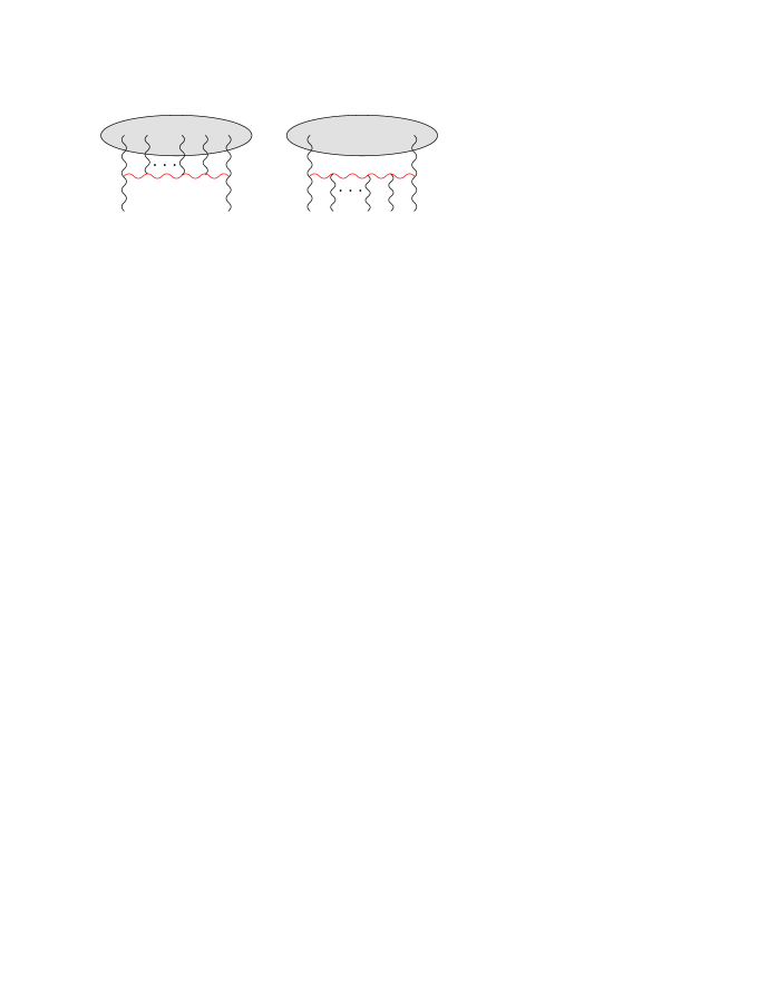
Figure 13: Vertices of JIMWLK and its dual.

In fact, close to the fluctuation line we defined earlier, the dipole density is of order $\mathcal{O}(1)$, and therefore charge densities are of order $\mathcal{O}(g)$ (of course $\langle\rho\rangle=0$ due to color neutrality, but $\langle\rho\rho\rangle=\mathcal{O}(g^{2})$ and so on). For the same reasons, in the JIMWLK evolution there was not such an issue, since $\rho$ was always much bigger than $g$, and the commutator was subleading. Now the evolution equation for an appropriate observable $\mathcal{O}$ may be written in the form

$$\frac{\partial\langle\mathcal{O}\rangle}{\partial Y}=\langle[\bar{H},\mathcal{O}]\rangle.$$ (72)

Based on the above considerations, it becomes obvious that if we consider gauge invariant observables built from the temporal Wilson lines in the fundamental representation, and starting from ${\rm tr}(W_{\bm{x}}W^{{\dagger}}_{\bm{y}})$, we shall generate the dual of the Balitsky hierarchy. This is not so surprising after all, since the diagram on the right part of Fig. 13 when viewed upside-down corresponds to the JIMWLK evolution of a left mover, while the correlators of the temporal Wilson lines correspond to the amplitudes for right movers to scatter of these evolved left movers. But of course this trivial aspect is not what we were looking for, rather we are interested to see how $\bar{H}$ can describe the low density fluctuations. Before that, and as a first check, one can see that Eq. (72), with $\mathcal{O}$ the bilinear of the charge density as defined in Eq. (64), will lead to the BFKL equation for the dipole density of the target hadron. To measure the fluctuations we need to consider a higher order correlator of charges, for example the dipole pair density $\bar{n}_{\bm{u}_{1}\bm{v}_{1}}\bar{n}_{\bm{u}_{2}\bm{v}_{2}}$ with $\bar{n}$ defined in Eq. (64). Here, one will obtain Eq. (45) but there will be additional terms to the right hand side of the equation. The same will happen if we consider the scattering of two projectile dipoles in order to probe these fluctuations; acting with $\bar{H}$ on $T_{\bm{x}_{1}\bm{y}_{1}}T_{\bm{x}_{2}\bm{y}_{2}}$ at the two-gluon exchange approximation, we obtain the normal BFKL evolution terms, the splitting term in Eq. (50) plus additional terms. Some of these terms will be suppressed in the large-$N_{c}$ limit, but some will not. For example there will be terms which correspond to the simultaneous scattering off the same target dipole, and this process is not subdominant in the multi-color limit. More generally the two dipoles could scatter off more complicated combinations of the target color sources.

One may have already seen that there are some subtleties associated with the dual Hamiltonian and the particular observables that we are interested in. Since the color charges are non-commutative, one has a difficulty in defining the observables at equal time $x^{+}$. For example, even though there is no problem with the single dipole density, since $[\rho^{a}_{\bm{u}},\rho^{a}_{\bm{v}}]=0$, there is an ambiguity in defining the dipole-pair density since $[\bar{n}_{\bm{u}_{1}\bm{v}_{1}},\bar{n}_{\bm{u}_{2}\bm{v}_{2}}]\neq 0$ and similarly for the dipole-pair scattering amplitude, since the color field $\alpha^{a}$ is related to the charge $\rho^{a}$ through the solution of the Poisson equation. Thus one needs a prescription to circumvent the problem, for example by considering symmetrized observables.

Of course these difficulties should disappear when one assumes that the target be composed of dipoles. The dipoles are color neutral, and therefore there should be no non-commutativity issues any more. In that case, one may ask if the dual Hamiltonian $\bar{H}$ will reduce to $H^{{\dagger}}_{1\to 2}$ in Eq. (63) since the latter was derived on the basis of the dipole picture. But one cannot really answer this question, since the assumption that the relevant degrees of freedom are dipolar, is a condition to be imposed on the wavefunction of the system and is not a property of the Hamiltonian. So let us assume that the wavefunction is of the form

$$Z_{Y}[\rho]=\sum_{N=1}^{\infty}\int{\rm d}\Gamma_{N}\,P_{N}(\{z_{\imath}\};Y)\prod_{\imath=1}^{N}\frac{1}{N_{c}}\,{\rm tr}\big{(}W_{\bm{z}_{\imath-1}}W^{{\dagger}}_{\bm{z}_{\imath}}\big{)}\delta(\rho),$$ (73)

with the notation introduced in Sec. 9. Now in order to find the evolution equation of $\langle\mathcal{O}\rangle$, it is much easier to obtain first the evolution of the wavefunction $Z_{Y}[\rho]$, then multiply with $\mathcal{O}$ and finally integrate over $\rho$. When we apply this procedure to the dipole-pair density we obtain the standard evolution equation given in Eq. (45), provided that during the calculation we drop terms which are suppressed in the multi-color limit [116, 117, 118]. Still, this description contains more than the one given by $H^{{\dagger}}_{1\to 2}$. In the latter, only two gluons could be radiated from each color dipole in the wavefunction of the target, while in the former there is no such restriction and a dipole can radiate an arbitrary number of gluons. In particular, this means that two projectile dipoles are allowed to scatter off the same target dipole.

14 Effective Action

The next natural task should be to construct an effective theory which takes into account all the vertices describing $m\to n$ transitions, with $m$ and $n$ arbitrary (and greater or equal to 2), like the generic one appearing in Fig. 14. Whether this is the full set of vertices contributing at the leading logarithmic level in $\bar{\alpha}_{s}\ln(1/x)$ or not (presumably not), is a separate issue and if not it could turn out that the search for the “final solution” be a formidable and too ambitious task. In any case, it seems reasonable to avoid the discussion of this problem here.

The diagram in Fig. 14, and in the spirit of the CGC approach, corresponds to the propagation of a semi-fast gluon (the horizontal red gluon) in the presence of two types of background fields, and it represents the modes that we need to integrate as we go to higher and higher values of rapidity. The two background fields (in the Coulomb gauge) are the $A^{+}$ component of the color field, represented by the vertical gluons above the semi-fast one, and the radiative part of the $A^{-}$ component, represented by the vertical gluons below the semi-fast one. The semi-fast gluon will be slow with respect to the $A^{+}$ component of the background field, so it will appear to the latter as moving fast to the positive $x^{-}$ direction. Thus it will couple to that component through a Wilson line in the longitudinal direction. Similarly, it will be fast with respect to the $A^{-}$ component, it will appear to the latter as moving fast in the positive $x^{+}$ direction, and thus it will couple to that component through a Wilson line in the temporal direction. Therefore, and not surprisingly, both types of Wilson lines which we encountered (separately) in the cases of the JIMWLK Hamiltonian and its dual will appear in the final form of our effective action, and in fact these will be the only degrees of freedom.

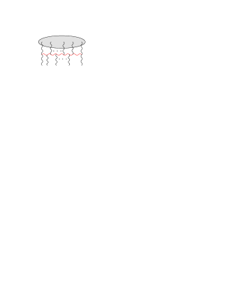
Figure 14: Generic vertex for an $m\to n$ transition.

In our current notation these Wilson lines in the adjoint representation (and by dropping the tilde we have been using so far) will read

$$\!\!\!\!\!\!V^{\dagger}_{x^{+}}(\bm{x})={\rm P}\,\exp\left[{\rm i}\,g\int\limits_{-\infty}^{\infty}{\rm d}x^{-}A^{+}_{a}(x^{+},x^{-},{\bm{x}})\,T^{a}\right],$$ (74)

$$\!\!\!\!\!\!W_{x^{-}}(\bm{x})={\rm P}\,\exp\left[{\rm i}\,g\int\limits_{-\infty}^{\infty}{\rm d}x^{+}A^{-}_{a}(x^{+},x^{-},{\bm{x}})\,T^{a}\right].$$ (75)

Again we will just present the final result for the change of the effective action under a rapidity step, and it can be given in the form [44]

$$\frac{\Delta S_{\rm eff}}{\Delta Y}=\frac{{\rm i}}{2\pi g^{2}N_{c}}\int\limits_{\bm{x}}{\rm Tr}\left[V^{\dagger}_{\infty}(\partial^{i}W_{-\infty})(\partial^{i}V_{-\infty})W^{\dagger}_{\infty}\right]\,\,+\,\,{\rm perm},$$ (76)

where “perm” stands for the three more terms arising from the possible permutations in the position of the spatial derivatives, and with the indices in the longitudinal and temporal Wilson lines standing for their $x^{+}$ and $x^{-}$ dependence respectively, in accordance with their definitions given above. This expression for the effective action has also been obtained in [45] by studying the scattering of two “shock waves” as developed in [119], while an earlier stage of the same expression has been reached in [42]. The four Wilson lines are not independent, rather they satisfy the constraint

$$V^{\dagger}_{\infty}W_{-\infty}V_{-\infty}W^{\dagger}_{\infty}=1\Rightarrow\frac{1}{N_{c}^{2}-1}\,{\rm Tr}\,W_{\diamondsuit}=1,$$ (77)

where $W_{\diamondsuit}$ is the Wilson loop shown in Fig. 15.

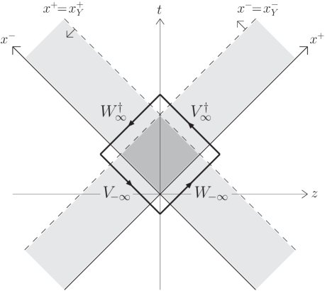
Figure 15: Wilson lines and the distribution of the background color fields in the $x^{+}-x^{-}$ plane.

This loop encloses the diamond defining the “interaction” area; the color field $A^{+}$ has support in the strip $0\leq x^{-}\leq x_{Y}^{-}\sim x_{0}^{-}{\rm e}^{Y}$ and its width expands with increasing rapidity, while the color field $A^{-}$ has support in the strip $0\leq x^{+}\leq x_{Y}^{+}\sim x_{0}^{+}{\rm e}^{-Y}$ and its width contracts with increasing rapidity. Notice that the value of the effective action in Eq. (76) depends only on the value of the fields on the boundary of this diamond-shaped area, and therefore it seems that the high energy problem reduces to a two-dimensional effective theory. Of course, at the same time, one will not be able to probe $x^{-}$ and/or $x^{+}$ dependent correlations of the system (but this was the case in both JIMWLK and its dual anyway), since the construction of $S_{\rm eff}$ results in a coarse-graining along these longitudinal and temporal directions.

This effective action is invariant under duality transformations as anticipated [44]. Indeed, if we let

$$W_{\infty}\rightarrow V^{{\dagger}}_{\infty},\qquad W_{-\infty}\rightarrow V^{{\dagger}}_{-\infty},$$ (78)

$S_{\rm eff}$ transforms to an expression which is fully equivalent to the one given in Eq. (76). Furthermore, the effective action will reduce to known expressions in limiting cases. Expanding the temporal Wilson lines to lowest non-trivial order, integrating over $x^{+}$, letting $A^{-}\!\to-{\rm i}\delta/\delta\rho$ and using the Poisson equation to relate $\rho$ to $A^{+}\equiv\alpha$, one obtains the JIMWLK Hamiltonian as given in Eq. (19). Similarly, an expansion of the longitudinal Wilson lines leads to the dual of JIMWLK as given in Eq. (68).

However, we should stress that Eq. (76) is not the complete answer to our problem. What we would really like to have is a Hamiltonian, that is, the effective action should be accompanied by well-defined commutators satisfied by its degrees of freedom, i.e. the Wilson lines. Then we would be able to find how the wavefunction of the system and the average values of the observables evolve with rapidity, as we did in the two limiting (JIMWLK and its dual) cases. For example, we have not been able to do the “simplest” but most natural exercise; to write the evolution equations obeyed by the dipole scattering amplitudes in this general case where all $m\to n$ transitions are possible, as this would allow us to generalize the hierarchy presented in Sec. 10. This problem is still “open” and therefore we shall not discuss it here. Let us just mention that the simple rule $A^{-}\to-{\rm i}\delta/\delta\rho$ for promoting an action into a Hamiltonian, and which is valid in the two limiting cases, will presumably not work any more. First of all, $A^{-}$ is not the natural degree of freedom, rather the latter is given by the corresponding temporal Wilson line. Furthermore, a replacement like the one mentioned above would lead to commutators which depend on “broken” Wilson lines (lines in, say $x^{-}$, which run from $-\infty$ to an upper limit different than $\infty$), a feature that makes the whole approach ill-defined.

15 The Saturation Momentum Revisited

In this last section we shall try to find the corrections in the energy dependence of the saturation momentum, which are induced by the splitting terms in the evolution equations. The result will be the one found in [34], even though we shall present a much simpler calculation while at the same time we will attempt to “improve” it. As was claimed in [34] and in Sec. 7, one needs to introduce an ultraviolet absorptive boundary to cut all the contributions from the region where the amplitude is such that $T\lesssim\alpha_{s}^{2}$, since they correspond to unitarity violating paths. Put it another way, a splitting of Pomerons in the target point of view, corresponds to a merging of Pomerons in the projectile point of view and therefore this boundary is like a saturation boundary for the projectile. The result of [34] has also been confirmed in [35], by identifying and studying the analogy to a similar problem in statistical physics. Indeed, as we saw in Sec. 10, the full large-$N_{c}$ hierarchy can be reduced, under certain but justified for our purposes approximations, to a Langevin problem [38] which is similar to the sFKPP equation. This equation shares the same features as the, deterministic, FKPP equation, when the latter is supplied with a cutoff at $\alpha_{s}^{2}$.

Therefore we would like to solve the BFKL equation with two absorptive boundaries. The separation, in logarithmic units, between these two boundaries, the saturation line and the fluctuation line, should be

$$\Delta=\frac{1}{1-\gamma_{\rm r}}\,\ln\frac{1}{\alpha_{s}^{2}}+\mathcal{O}(\rm const),$$ (79)

as shown in Fig. 6, since within $\Delta$ the amplitude will drop from a value of order $\mathcal{O}(1)$ to a value of order $\mathcal{O}(\alpha_{s}^{2})$, as determined from its leading power behavior in $Q^{2}$ (in Eq. (79) we have anticipated that the real part of the anomalous dimension will not be $\gamma_{s}$ any more and its value $\gamma_{\rm r}$ is to be determined). The constant in Eq. (79) is not really under control, since it can be affected, for example, by the precise value of $T$ on the boundaries. Even though this constant should not affect the leading correction, since it is suppressed with respect to the leading term when $\alpha_{s}\to 0$, it will turn out to have an important influence on the results for small, but reasonable, values of the coupling constant.

By making a change of variables, from $(\ln(Q^{2}/\mu^{2}),Y)$ to $(z,Y)$, with $z\equiv\ln(Q^{2}/Q_{s}^{2}(Y))$, one can write the BFKL equation as

$$\left[\chi\left(1+\frac{\partial}{\partial z}\right)-\lambda_{s}\,\frac{\partial}{\partial z}\right]T=0.$$ (80)

The above expression has been set equal to zero, instead of $(1/\bar{\alpha}_{s})\,\partial T/\partial Y$, since we are looking for lines of constant scattering amplitude $T$, that is, $Y$-independent solutions for $T$. In Eq. (80), $\lambda_{s}$ is the logarithmic derivative of the saturation momentum, which is to be determined. Now let us recall that the BFKL eigenfunctions are exponentials in $z$, where the anomalous dimension is in general complex, i.e. $\gamma=\gamma_{\rm r}+{\rm i}\,\gamma_{{\rm i}}$, with obvious notation. Then one can see that the unique real linear combination of eigenfunctions, which satisfies the boundary conditions $T(z=0)=T(z=\Delta)=0$ is

$$T\propto\exp[-(1-\gamma_{\rm r})\,z]\sin\frac{\pi z}{\Delta}.$$ (81)

In the above equation the sine has been obviously generated by the linear combination of the parts of the two degenerate eigenfunctions that involve the complex piece of the anomalous dimension, which is uniquely determined in terms of $\Delta$ and reads $\gamma_{{\rm i}}=\ \pi/\Delta$. Furthermore, in order for Eq. (81) to satisfy Eq. (80) and since the saturation momentum is a real quantity, the constant $\lambda_{s}$ must be given by

$$\lambda_{s}=\frac{\chi(\gamma)}{1-\gamma}\qquad{\rm with}\qquad{\rm Im}(\lambda_{s})=0.$$ (82)

This last equation is the solution to our problem, since for a given value of $\gamma_{{\rm i}}$ (that is, for a given $\Delta$ or for a given $\alpha_{s}$), there will be a unique value of the real part $\gamma_{\rm r}$ of the anomalous dimension which makes the logarithmic derivative of the saturation momentum $\lambda_{s}$ real. Notice that the solution will not correspond to a saddle point of $\chi(\gamma)/(1-\gamma)$, in contrast to the single boundary case, cf. Eq. (31).

When the separation of the boundaries is large, or equivalently the coupling is extremely small, i.e. $\Delta\gg 1\Leftrightarrow\alpha_{s}\ll 1$, we can expand the r.h.s. of Eq. (82) around the asymptotic anomalous dimension which is $\gamma_{s}$ as expected and as shown in Fig. 16. By setting the imaginary part of this expansion equal to zero, we uniquely determine $\gamma_{\rm r}$ and then the real part gives $\lambda_{s}$. It is not hard to find that in this expansion the logarithmic derivative of the saturation momentum is given by [34]

$$\frac{\lambda_{s}}{\bar{\alpha}_{s}}=\frac{\chi(\gamma_{s})}{1-\gamma_{s}}-\frac{\pi^{2}(1-\gamma_{s})\chi^{\prime\prime}(\gamma_{s})}{2\ln^{2}(\alpha_{s}^{2})}=4.88-\frac{150}{\ln^{2}(\alpha_{s}^{2})},$$ (83)

while the real part of the anomalous dimension reads

$$\gamma_{\rm r}=\gamma_{s}+\left[1+\frac{(1-\gamma_{s})\chi^{\prime\prime\prime}(\gamma_{s})}{3\chi^{\prime\prime}(\gamma_{s})}\right]\frac{\pi^{2}(1-\gamma_{s})}{2\ln^{2}(\alpha_{s}^{2})}=0.372-\frac{0.562}{\ln^{2}(\alpha_{s}^{2})}.$$ (84)

It is obvious that as we let the second boundary to infinity, i.e. when $\alpha_{s}\to 0$, we approach the results of the single boundary problem. The same is true for the scattering amplitude too; as $\Delta\to\infty$, Eq. (81) reduces to the scaling part (the first two factors) of Eq. (33). Of course it is not surprising that the correction in $\lambda_{s}$ is negative, since there is absorption from the two boundaries. Moreover, we should notice that the denominator in the correction of $\lambda_{s}$ has again a simple interpretation; it is proportional to the square of the “effective” transverse phase space, in logarithmic units, for the evolution of the system, which here is $\Delta^{2}\sim\ln^{2}(\alpha_{s}^{2})$, as it was in the single boundary case (cf. Eq. (32) and the discussion after that). A rather important feature of these corrections, which are generated in reality by the negative contribution of the Pomeron loops formed in the course of the evolution, is that they appear to be much more significant that any next to leading order correction; indeed the latter would simply add a term of order $\mathcal{O}(\alpha_{s})$ with respect to the leading term.

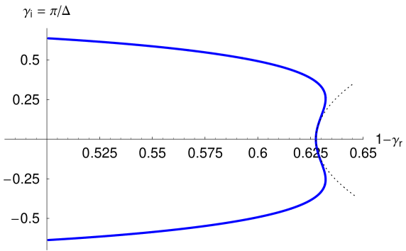
Figure 16: The anomalous dimension in the two boundary approximation (with the thin dotted line corresponding to Eq. (84)).

These corrections have the nice feature that they are universal, that is, they do not depend on the precise width of the boundary. If we let $\alpha_{s}\to\kappa\alpha_{s}$, with $\kappa=\mathcal{O}(1)$, which amounts to the modification of the boundary width by an additive constant, the induced correction in Eqs. (83) and (84) will be of order $\mathcal{O}(1/\ln^{3}(\alpha_{s}^{2}))$. But within the same reasoning, these equations are as far as one can go by using analytical methods, since any higher order correction will depend on the precise value of the boundary width, and thus one cannot rely on the BFKL equation any more.

This brings us in a somewhat difficult situation, since the coefficient in the correction of $\lambda_{s}$ is huge, mostly due to the large value of $\chi^{\prime\prime}(\gamma_{s})$. Indeed, for reasonable values of $\alpha_{s}$ the correction will dominate the leading contribution; $\lambda_{s}$ as given in Eq. (83) will be negative so long as $\alpha_{s}\gtrsim 0.06$. Of course this does not mean that there is something wrong neither with Eq. (83) nor with the problem at hand. Eq. (83) is really supposed to be valid at very small $\alpha_{s}$, while for a realistic value of $\alpha_{s}$ we should rely on a (numerical) solution of the full set of equations, i.e. including non-linearities and fluctuations.

One can already see that the situation will be better if we decide not to expand the BFKL kernel in the diffusion approximation, as we did while going from Eq. (82) to Eq. (83). Eq. (82) is just an algebraic equation which can be easily solved numerically for a given, but arbitrary, value of $\alpha_{s}$. In Fig. 16 we show the solution for the anomalous dimension in the complex plane, while in Fig. 17 we show the dependence of $\lambda_{s}/\bar{\alpha}_{s}$ on $\alpha_{s}$.

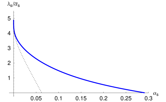
Figure 17: The logarithmic derivative of the saturation momentum in the two boundary approximation (with the thin dotted line corresponding to Eq. (83)).

As we see in Fig. 16 and also in Eq. (84) there is an important correction to the real part of the anomalous dimension, but not as huge as in the case of $\lambda_{s}$. It is amusing, but also natural, that there is no solution for values of $\gamma$ such that $\gamma_{\rm r}\geq\gamma_{\mathbb{P}}=1/2$. This is the point where the saturation line becomes identical to the Pomeron intercept line. That means that the latter becomes a line of constant amplitude (like the saturation line); the negative corrections induced by the boundaries will exactly cancel the leading value $\omega_{\mathbb{P}}=4\bar{\alpha}_{s}\ln 2$. Since the Pomeron intercept line corresponds to the line of fastest increase, we conclude that there will be no high energy growth any more, therefore no saturation, and thus no solution to our problem!

In Fig. 17 we see that $\lambda_{s}$ starts from the, well-known by now, asymptotic value $4.88\bar{\alpha}_{s}$ for vanishing $\alpha_{s}$ and it decreases to become zero at a point which is of course the same as the point in Fig. 16 where $\gamma_{\rm r}=1/2$ and there is no solution any more. The change in the “speed” of the saturation momentum is still significant, but the total result is positive in a much wider region of possible values of $\alpha_{s}$, more precisely one has $\lambda_{s}(\alpha_{s}\lesssim 0.3)>0$. Of course this is not really under control, since one is free to rescale $\alpha_{s}$ by a factor of order $\mathcal{O}(1)$. Nevertheless, this result behaves much better than Eq. (83), while both are solutions to the same problem and under the same definition for the boundary width $\Delta$ as a function of $\alpha_{s}$. Thus, one expects that in a (numerical) solution of the full problem, the outcome will presumably be well-defined for all reasonable values of the coupling constant.

Our presentation would be incomplete, if at this point we would not mention that the scaling behavior of the amplitude will not persist at very high values of rapidity [34] due to the presence of the fluctuations terms in the evolution equations [35, 38]. Since the system is of stochastic nature, different events will lead to different profiles of the scattering amplitude as a function of $Q^{2}$ and at a given fixed rapidity $Y$ [35]. These profiles will be of the same form but shifted with respect to each other according to a probability density, which at a first approximation can be taken as a Gaussian with a diffusive radius which scales as $\scriptstyle{\sqrt{\textstyle{\bar{\alpha}_{s}Y/\ln^{3}(1/\alpha_{s}^{2})}}}$. Averaging over all the events, one finds that [35]

$$\langle T(Q^{2},Y)\rangle=F\left(\frac{\ln(Q^{2}/\langle Q_{s}^{2}\rangle)}{\scriptstyle{\sqrt{\textstyle{\bar{\alpha}_{s}Y/\ln^{3}(1/\alpha_{s}^{2})}}}}\right),$$ (85)

which clearly violates the geometrical scaling of the amplitude. Such violations, and their consequences, for instance the breakdown of the BFKL approximation in the high momentum region [38], have been seen in the existing numerical solutions [112, 113], but the precise value of the critical rapidity that they set in (which could depend on the initial conditions) is not under real control yet.

16 Epilogue

In these lectures I have tried to give a simple introduction (and not only) to the basic theoretical developments, during the last decade or so, in the field of high energy (small-$x$) QCD. To this end, I have introduced, and relied mostly to, the dipole picture of high energy evolution and the Color Glass Condensate formulation of an energetic hadron, since, to my opinion, these are the simplest and perhaps most promising self-consistent approaches to the problem. Even though I have not followed a step by step procedure in the construction of the effective theory governing the dynamics at this high-energy limit, I have tried to describe as much as possible the underlying physical picture, and in the Appendices that follow I give the derivations of some relevant equations in order to have a more complete presentation.

I feel that we have seen important progress in the field during the last year, since we were able to derive evolution equations containing Pomeron loops as one of their building blocks, which is really the mechanism that eventually leads to the unitarization of scattering amplitudes and the saturation of hadronic wavefunctions (even though for an accurate description of the latter one may need to go beyond the large-$N_{c}$ limit).

Of course there are still many open questions and things to be done. For instance, it would be natural to look for the extension of the evolutions equations to finite-$N_{c}$ which allow transitions among arbitrary numbers of Pomerons, even though the solution of such generalized equations may turn out to be not much different for most interesting quantities (in the same way that the BK and JIMWLK equations share, at some level, the same features). So, at the moment, we would like to have a better analytical insight to the current set of equations, and presumably this can be achieved by analyzing their stochastic nature, while at the same time more accurate solutions are needed. Clearly this is rather important if one aims to see the implications at the phenomenological level. To this purpose, and for a more complete analysis, one would really like to go beyond this hierarchy, which is good for the description of total cross sections, and extend it, if possible, to the case of diffractive scattering (such attempts, but restricted to BK and/or JIMWLK evolution have been already made [122, 123, 124]). On the theoretical side, I believe that it is important to investigate the relationship with the other approaches to the problem and the possible equivalence between them, so that at the end of the day one will have a unified and concrete description of the dynamics in high-energy QCD.

Appendix A The Dipole Kernel

In this Appendix we will derive the expression given in Eq. (2) for the dipole emission kernel [5]. Let us look at the left diagram in Fig. 18, where a soft gluon is emitted by the quark line. With the 4-momenta of the quark and the gluon being $p^{\mu}=(p^{-}\!=\bm{p}^{2}/2p^{+}\!\to\!0,p^{+}\!\!\to\!\infty,\bm{p}\!\to\!\bm{0})$ and $k^{\mu}=(k^{-}=\bm{k}^{2}/2k^{+},k^{+}=xp^{+},\bm{k})$ respectively, the probability amplitude for this emission in light-cone old fashioned perturbation theory is given by

$$\mathcal{M}_{\lambda}^{a}(k^{+},\bm{k})=\frac{g\,t^{a}\epsilon_{\lambda}^{-}}{\sqrt{(2\pi)^{3}2k^{+}}}\,\frac{1}{k^{-}}=\frac{2g\,t^{a}}{\sqrt{(2\pi)^{3}2k^{+}}}\,\frac{\bm{\epsilon}_{\lambda}\!\cdot\!\bm{k}}{\bm{k}^{2}}.$$ (86)

Here, $\lambda$ stands for the polarization of the gluon, $g\,t^{a}\epsilon_{\lambda}^{-}$ is the quark gluon vertex in the high energy approximation, $1/k^{-}$ corresponds to the energy denominator which is dominated by the gluon, and the square root factor arises from the usual normalization of the color field. We have also used the fact that, in the light cone gauge $A^{+}=0$, the condition $k_{\mu}\epsilon_{\lambda}^{\mu}=0$ implies $\epsilon_{\lambda}^{-}=\bm{\epsilon}_{\lambda}\!\cdot\!\bm{k}/k^{+}$. It is straightforward to perform a Fourier transformation in order to obtain the probability amplitude in transverse coordinate space, which reads

$$\mathcal{M}_{\lambda}^{a}(k^{+},\bm{x}\!-\!\bm{z})= \!\!\!\!\!\!\int\limits_{\bm{k}}\frac{\exp\left[{\rm i}\bm{k}\!\cdot\!(\bm{x}\!-\!\bm{z})\right]}{(2\pi)^{2}}\,\mathcal{M}_{\lambda}^{a}(k^{+},\bm{k})$$

$$= \!\!\!\!\!\!\frac{1}{2\pi}\,\frac{2{\rm i}g\,t^{a}}{\sqrt{(2\pi)^{3}2k^{+}}}\,\frac{\bm{\epsilon}_{\lambda}\!\cdot\!(\bm{x}\!-\!\bm{z})}{(\bm{x}\!-\!\bm{z})^{2}}.$$ (87)

Similarly the probability amplitude for emission from the antiquark line of the dipole will be $\mathcal{M}_{\lambda}^{a}(k^{+},\bm{z}\!-\!\bm{y})$. Then the differential emission probability in the interval ${\rm d}^{2}\bm{z}$ and from $k^{+}$ to $k^{+}\!-{\rm d}k^{+}$ (we anticipate that the change in the probability will be positive when $k^{+}$ decreases and therefore the longitudinal phase space “opens up”) will be given by

$${\rm d}P=-(2\pi)^{2}\sum_{a,\lambda}\left|\mathcal{M}_{\lambda}^{a}(k^{+},\bm{x}\!-\!\bm{z})+\mathcal{M}_{\lambda}^{a}(k^{+},\bm{z}\!-\!\bm{y})\right|^{2}{\rm d}^{2}\bm{z}\,{\rm d}k^{+}.$$ (88)

The factor $(2\pi)^{2}$ arises when we transform the (square of the) wavefunction of the initial state in momentum space to the one in coordinate space. By using $t^{a}t^{a}=(N_{c}^{2}-1)/(2N_{c})\to N_{c}/2$ to sum over color indices in the large-$N_{c}$ limit, and $\sum_{\lambda}\epsilon_{\lambda}^{\imath}\epsilon_{\lambda}^{*\jmath}=\delta^{\imath\jmath}$ to sum over polarization indices, we finally arrive at

$${\rm d}P=\frac{\bar{\alpha}_{s}}{2\pi}\,\frac{(\bm{x}-\bm{y})^{2}}{(\bm{x}-\bm{z})^{2}(\bm{z}-\bm{y})^{2}}\,{\rm d}^{2}\bm{z}\,{\rm d}Y.$$ (89)

In the above equation, we have introduced the rapidity increment ${\rm d}Y$. Notice that this factor arises from the longitudinal phase space $-{\rm d}k^{+}/k^{+}=-{\rm d}x/x={\rm d}\ln(1/x)={\rm d}Y$.

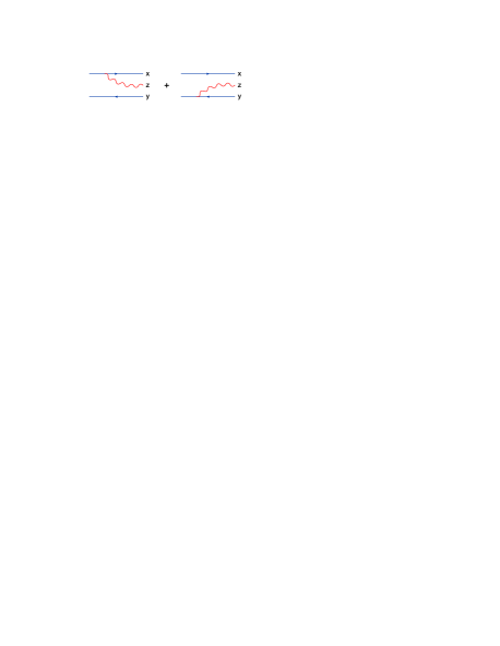
Figure 18: The two diagrams contributing to the splitting amplitude.

Appendix B The Elementary Dipole-Dipole Scattering Amplitude

Here we will calculate the imaginary part of the dipole-dipole scattering amplitude in the two-gluon exchange approximation. In this limit only tree diagrams need to be considered and one can simply use classical field equations. Let us assume that the dipole $(\bm{u},\bm{v})$ creates a field $\alpha^{a}$ which is “seen” from the dipole $(\bm{x},\bm{y})$. In general, the amplitude for the dipole $(\bm{x},\bm{y})$ to scatter off a classical field $\alpha^{a}$ is determined by

$$T(\bm{x}\bm{y}|\alpha)=\frac{g^{2}}{4N_{c}}\,\big{[}\alpha^{a}(\bm{x})-\alpha^{a}(\bm{y})\big{]}^{2}.$$ (90)

When this field is created by a source $\rho^{a}$, it can be determined by the solution of the Poisson equation in the Coulomb gauge, more precisely

$$\nabla_{\bm{z}}^{2}\alpha^{a}(\bm{z})=-\rho^{a}(\bm{z})\,\,\Longrightarrow\,\,\alpha^{a}(\bm{z})=-\frac{1}{4\pi}\int\limits_{\bm{w}}\ln\big{[}(\bm{z}-\bm{w})^{2}\mu^{2}\big{]}\rho^{a}(\bm{w}).$$ (91)

Then Eq. (90) becomes

$$T(\bm{x}\bm{y}|\rho)=\frac{g^{2}}{64\pi^{2}N_{c}}\left[\int\limits_{\bm{w}}\ln\bigg{[}\frac{(\bm{x}-\bm{w})^{2}}{(\bm{y}-\bm{w})^{2}}\bigg{]}\,\rho^{a}(\bm{w})\right]^{2}.$$ (92)

In the problem under consideration the source consists of the quark and the antiquark of the dipole $(\bm{u},\bm{v})$, and therefore its charge is given by

$$\rho^{a}(\bm{w})=g\,t^{a}\left[\delta(\bm{w}-\bm{u})-\delta(\bm{w}-\bm{v})\right].$$ (93)

Substituting the expression (93) into Eq. (92) and by making use of

$$t^{a}t^{a}=\frac{N_{c}^{2}-1}{2N_{c}},$$ (94)

we finally arrive at

$$T_{0}(\bm{x}\bm{y}|\bm{u}\bm{v})=\frac{\alpha_{s}^{2}}{8}\,\frac{N_{c}^{2}-1}{N_{c}^{2}}\,\ln^{2}\left[\frac{(\bm{x}-\bm{v})^{2}(\bm{y}-\bm{u})^{2}}{(\bm{x}-\bm{u})^{2}(\bm{y}-\bm{v})^{2}}\right].$$ (95)

Notice that this is invariant under the exchange of the two dipoles, i.e. $\bm{x}\bm{y}\leftrightarrow\bm{u}\bm{v}$ and under the exchange of the quark and the antiquark within the same dipole, i.e. $\bm{x}\leftrightarrow\bm{y}$ and/or $\bm{u}\leftrightarrow\bm{v}$. The latter will not be true, in general, when we relax the two-gluon exchange approximation.

One can also integrate over the impact parameter of the scattering, i.e. over the relative distance $\bm{b}=(\bm{x}\!+\bm{y}\!-\!\bm{u}\!-\!\bm{v})/2$ between the two dipoles, average over the orientation of the two dipoles, and multiply by a factor of 2 to obtain a total cross section

$$\sigma_{\rm DD}(r_{1},r_{2})=2\pi\alpha_{s}^{2}\,r_{<}^{2}\bigg{(}1+\ln\frac{r_{>}}{r_{<}}\bigg{)}.$$ (96)

In the above equation $r_{1}$ and $r_{2}$ are the sizes of the two dipoles $(\bm{x},\bm{y})$ and $(\bm{u},\bm{v})$, $r_{<}={\rm min}(r_{1},r_{2})$ and $r_{>}={\rm max}(r_{1},r_{2})$, while we have also set the color factor equal to its large-$N_{c}$ value. When either of the dipole sizes vanishes, this total cross section vanishes due to color transparency.

Appendix C The BFKL Equation: From Dipole Densities to Scattering Amplitudes

The BFKL equation for the dipole density in the wavefunction of the target reads

$$\frac{\partial\langle n_{\bm{u}\bm{v}}\rangle}{\partial Y}=\frac{\bar{\alpha}_{s}}{2\pi}\int\limits_{\bm{z}}\big{[}{\mathcal{M}}_{\bm{u}\bm{z}\bm{v}}\langle n_{\bm{u}\bm{z}}\rangle+{\mathcal{M}}_{\bm{z}\bm{v}\bm{u}}\langle n_{\bm{z}\bm{v}}\rangle-{\mathcal{M}}_{\bm{u}\bm{v}\bm{z}}\langle n_{\bm{u}\bm{v}}\rangle\big{]}.$$ (97)

In the two-gluon exchange approximation, the amplitude for a dipole $(\bm{x},\bm{y})$ to scatter of the target is given by a linear transformation of the dipole density, namely

$$\langle T_{\bm{x}\bm{y}}\rangle=\int\limits_{\bm{u}\bm{v}}T_{0}(\bm{x}\bm{y}|\bm{u}\bm{v})\,\langle n_{\bm{u}\bm{v}}\rangle,$$ (98)

with $T_{0}(\bm{x}\bm{y}|\bm{u}\bm{v})$ the elementary dipole-dipole scattering amplitude at lowest order in perturbation theory, and when the color-factor is set to its large-$N_{c}$ value, one has (cf. Eq. (95))

$$T_{0}(\bm{x}\bm{y}|\bm{u}\bm{v})=\frac{\alpha_{s}^{2}}{8}\ln^{2}\left[\frac{(\bm{x}-\bm{v})^{2}(\bm{y}-\bm{u})^{2}}{(\bm{x}-\bm{u})^{2}(\bm{y}-\bm{v})^{2}}\right].$$ (99)

Differentiating Eq. (98) with respect to $Y$, using Eq. (97) and making some trivial interchanges of variables we obtain

$$\!\!\!\frac{\partial\langle T_{\bm{x}\bm{y}}\rangle}{\partial Y}=\frac{\bar{\alpha}_{s}}{2\pi}\!\int\limits_{\bm{u}\bm{v}\bm{z}}\!\mathcal{M}_{\bm{u}\bm{v}\bm{z}}\big{[}T_{0}(\bm{x}\bm{y}|\bm{u}\bm{z})+T_{0}(\bm{x}\bm{y}|\bm{z}\bm{v})\!-\!T_{0}(\bm{x}\bm{y}|\bm{u}\bm{v})\big{]}\langle n_{\bm{u}\bm{v}}\rangle.$$ (100)

Let us concentrate on the integration over $\bm{z}$, and make a change of variables through the conformal transformation

$$z\to\frac{z+c_{1}}{c_{2}\,z-1},$$ (101)

with the parameters $c_{1}$ and $c_{2}$ given by

$$c_{1}=-\frac{x^{-1}-y^{-1}+u^{-1}-v^{-1}}{(xu)^{-1}-(yv)^{-1}},\quad c_{2}=\frac{x-y+u-v}{xu-yv},$$ (102)

and where we have defined the complex variable $z=z_{1}+{\rm i}\,z_{2}$, with $\bm{z}=(z_{1},z_{2})$ (and similarly for $\bm{x},\bm{y},\bm{u},\bm{v}$). This particular transformation for $\bm{z}$ does not change the functional form of the integrand, composed of the dipole kernel, the square bracket and the integration measure ${\rm d}^{2}\bm{z}$, but simply performs the mapping $\bm{x}\leftrightarrow\bm{u}$ and $\bm{y}\leftrightarrow\bm{v}$. Therefore Eq. (100) becomes

$$\!\!\!\frac{\partial\langle T_{\bm{x}\bm{y}}\rangle}{\partial Y}=\frac{\bar{\alpha}_{s}}{2\pi}\!\int\limits_{\bm{u}\bm{v}\bm{z}}\!\mathcal{M}_{\bm{x}\bm{y}\bm{z}}\big{[}T_{0}(\bm{x}\bm{z}|\bm{u}\bm{v})+T_{0}(\bm{z}\bm{y}|\bm{u}\bm{v})\!-\!T_{0}(\bm{x}\bm{y}|\bm{u}\bm{v})\big{]}\langle n_{\bm{u}\bm{v}}\rangle,$$ (103)

and now by making use of Eq. (98), we finally arrive at the equation describing the scattering amplitude of a single projectile dipole off the target in the BFKL approximation which reads

$$\frac{\partial\langle T_{\bm{x}\bm{y}}\rangle}{\partial Y}=\frac{\bar{\alpha}_{s}}{2\pi}\int\limits_{\bm{z}}\mathcal{M}_{\bm{x}\bm{y}\bm{z}}\big{[}\langle T_{\bm{x}\bm{z}}\rangle+\langle T_{\bm{z}\bm{y}}\rangle-\langle T_{\bm{x}\bm{y}}\rangle\big{]}.$$ (104)

Appendix D Eigenvalues of the BFKL Equation

Here we shall find the eigenvalues of the BFKL equation in the simplified case where the scattering amplitude satisfies $T_{\bm{x}\bm{y}}=T(r)$, where $r=|\bm{r}|\equiv|\bm{x}-\bm{y}|$ is the size of the dipole. The integration measure on the right hand side of Eq. (104) may be written as

$${\rm d}^{2}\bm{z}=2\pi r_{1}r_{2}{\rm d}r_{1}{\rm d}r_{2}\int\limits_{0}^{\infty}{\rm d}\ell\,\ell\,J_{0}(\ell r)J_{0}(\ell r_{1})J_{0}(\ell r_{2}),$$ (105)

with $r_{1}$ and $r_{2}$ the sizes of the child dipoles $(\bm{x},\bm{z})$ and $(\bm{z},\bm{y})$ respectively, and where $J_{0}$ is a Bessel function of the first kind. Then the right hand side of Eq. (104) (divided by $\bar{\alpha}_{s}$) becomes

$$\mathcal{K}_{\rm BFKL}^{\epsilon}\otimes T(r)\equiv\!\!\int\limits_{r_{1}r_{2}\ell}\!\!\frac{1}{r_{1}^{1-2\epsilon}}\,\frac{1}{r_{2}^{1-2\epsilon}}\,r^{2}\ell\, \!\!\!\!\!\!J_{0}(\ell r)J_{0}(\ell r_{1})J_{0}(\ell r_{2})$$ (106)

$$\!\!\!\!\!\!\times[T(r_{1})+T(r_{2})-T(r)],$$

with $\epsilon$ a positive regularization constant which at the end will be set equal to zero. Since there is no mass scale appearing in the BFKL equation and the kernel combined with the integration measure has no dimension, one expects the eigenfunctions to be pure powers of the dipole size $r$. Indeed, with $T(r)=r^{2(1-\gamma)}$ one can successively integrate over $r_{1}$, $r_{2}$ and $\ell$ in Eq. (106) to obtain

$$\mathcal{K}_{\rm BFKL}^{\epsilon}\!\!\otimes\!r^{2(1\!-\gamma)}\!\!=\!\frac{\Gamma(\epsilon)}{\Gamma(1\!-\!\epsilon)}\!\bigg{[}\frac{\Gamma(\gamma\!-\!2\epsilon)\Gamma(1\!+\!\epsilon\!-\!\gamma)}{\Gamma(\gamma\!-\!\epsilon)\Gamma(1\!+\!2\epsilon\!-\!\gamma)}\!-\!\frac{\Gamma\big{(}\frac{1}{2}\!-\!\epsilon\big{)}}{4^{\epsilon}\Gamma\big{(}\frac{1}{2}\!+\!\epsilon\big{)}}\bigg{]}r^{2(1\!-\gamma)+4\epsilon}.$$ (107)

Taking the limit $\epsilon\to 0$ one finds

$$\mathcal{K}_{\rm BFKL}\otimes r^{2(1-\gamma)}=\chi(\gamma)\,r^{2(1-\gamma)},$$ (108)

where

$$\chi(\gamma)=2\,\psi(1)-\psi(\gamma)-\psi(1-\gamma),$$ (109)

with $\psi(\gamma)$ the logarithmic derivative of the $\Gamma$-function, i.e.

$$\psi(\gamma)\equiv\frac{{\rm d}\ln\Gamma(\gamma)}{{\rm d}\gamma}.$$ (110)

An alternative, and perhaps easier, derivation may be given by noticing that the eigenvalue may be written as

$$\chi(\gamma)=\frac{1}{\pi}\int\limits_{\bm{z}}\frac{\bm{x}^{2}}{\bm{z}^{2}(\bm{x}-\bm{z})^{2}}\left(\frac{\bm{z}^{2-2\gamma}}{\bm{x}^{2-2\gamma}}-\frac{\bm{x}\!\cdot\!\bm{z}}{\bm{x}^{2}}\right),$$ (111)

where we have set $\bm{y}=\bm{0}$, we have used the fact that the first two terms in the BFKL equation give the same result and we have split the virtual term into two parts using $\bm{x}^{2}=\bm{x}\!\cdot\!\bm{z}-\bm{x}\!\cdot\!(\bm{z}\!-\!\bm{x})$, where both parts contribute equally. Now we can make the change of variable $z=xu$ to obtain

$$\chi(\gamma) \!\!\!\!\!\!=\frac{1}{\pi}\int\limits_{0}^{1}{\rm d}u\,\int\limits_{0}^{2\pi}{\rm d}\phi\,\frac{u^{1-2\gamma}+u^{2\gamma-1}-2\cos\phi}{1-2u\cos\phi+u^{2}}$$ (112)

$$\!\!\!\!\!\!=2\int\limits_{0}^{1}{\rm d}u\,\frac{u^{1-2\gamma}+u^{2\gamma-1}-2u}{1-u^{2}},$$

where we have transformed the integration over $u$ from $1$ to $\infty$ to an integration from $0$ to $1$, by letting $u\to 1/u$. Now the integration over $u$ leads to Eq. (109).

Appendix E The JIMWLK Hamiltonian

In this Appendix we “sketch” the derivation of the JIMWLK Hamiltonian. Let us decompose the field $A^{\mu}$ which is associated with the wavefunction of the energetic hadron as

$$A^{\mu}=B^{\mu}+a^{\mu}+\delta A^{\mu},$$ (113)

where $B^{\mu}$ is the background field generated by the source $\rho$, $a^{\mu}$ represents the semi-fast modes with longitudinal momenta such that $b\Lambda^{+}\ll|p^{+}|\ll\Lambda^{+}$ and with $b\ll 1$, while $\delta A^{\mu}$ contains modes with momenta $k^{+}\lesssim b\Lambda^{+}$. Since we want to measure expectation values of observables at scales below or equal to $b\Lambda^{+}$, we need to integrate the semi-fast modes $a^{\mu}$. Therefore we define an effective action as

$$S_{\rm eff}=-{\rm i}\ln\int\limits_{b\Lambda^{+}}^{\Lambda^{+}}\mathcal{D}\alpha\exp\left({\rm i}S\,[A,\rho]\right),$$ (114)

where the action $S\,[A,\rho]$ generates the classical field equations in the presence of a source $\rho$ (cf. Eq. (15)) when $\delta A^{\mu}=0$. The background field $B^{\mu}$ is determined by the solution to the Poisson equation. In the light-cone (LC) gauge, where only the transverse components are non-zero, i.e. $B^{\mu}=\delta^{\mu\imath}B^{\imath}$, we have

$$D_{\nu}F^{\nu+}=-D_{\imath}\,\partial^{+}B^{\imath}=\rho(x^{-},\bm{x}).$$ (115)

In writing the above equation we have used that $F^{-+}=-\partial^{+}\delta A^{-}\simeq 0$, which follows from the fact that $\delta A^{-}$ contains modes with very small longitudinal momenta and therefore it varies very slowly with $x^{-}$. We can write the solution to Eq. (115) as

$$B^{\imath}=\frac{{\rm i}}{g}\,\tilde{U}(x^{-},\bm{x})\,\partial^{\imath}_{\bm{x}}\,\tilde{U}^{{\dagger}}(x^{-},\bm{x}),$$ (116)

where the Wilson line $\tilde{U}^{{\dagger}}$ is given by

$$\tilde{U}^{{\dagger}}(x^{-},\bm{x})={\rm P}\exp\Bigg{[}{\rm i}\,g\int\limits_{-\infty}^{x^{-}}{\rm d}z^{-}\alpha^{a}(z^{-},\bm{x})\,T^{a}\Bigg{]},$$ (117)

and similarly for $U$. In the above equation $\alpha\equiv\hat{B}^{+}$ is the background field in the Coulomb gauge and, with $\hat{\rho}$ the corresponding Coulomb gauge source, it satisfies

$$\nabla_{\bm{x}}^{2}\,\alpha^{a}(x^{-},\bm{x})=-\hat{\rho}^{a}(x^{-},{\bm{x}}).$$ (118)

Notice that $B^{\imath}$ is a two-dimensional pure gauge, i.e. $F^{\imath\jmath}=0$. Now we expand the action $S$ around $A^{\mu}_{0}\equiv\delta^{\mu\imath}B^{\imath}+\delta^{\mu-}\delta A^{-}$ and to second order in the semi-fast modes $a^{\mu}$, that is

$$S=S_{0}+\frac{\delta S}{\delta A^{\imath}}\,a^{\imath}+\frac{1}{2}\,a^{\mu}\,G_{\mu\nu}^{-1}\,a^{\nu}.$$ (119)

The coefficient of the linear term may be written as

$$\frac{\delta S}{\delta A^{\imath}}=D_{\nu}F^{\nu\imath}=D_{\jmath}F^{\jmath\imath}+D^{+}F^{-\imath}+D^{-}F^{+\imath}\simeq 2D^{+}F^{-\imath},$$ (120)

where we have used the fact that $F^{\imath\jmath}=0$ and also the approximate equality $D^{-}F^{+\imath}\simeq D^{+}F^{-\imath}$. The latter arises from $\partial^{+}\delta A^{-}\simeq 0$ which was justified earlier just after Eq. (115). In the quadratic term in Eq. (119) $G_{\mu\nu}$ is the propagator in the presence of the background field $B^{\imath}$ (when calculating this propagator, the field $\delta A^{-}$ can be set equal to zero to the order of accuracy). Now we can perform the integration over the semi-fast modes $a^{\mu}$ to obtain the (change of the) effective action. It is given by the four-dimensional double integral

$$\Delta S_{\rm eff}=-\,\frac{1}{2}\int\limits_{xy}(2D^{+}F^{-\imath})_{x}\,G^{\imath\jmath}_{xy}\,(2D^{+}F^{-\imath})_{y}.$$ (121)

Up to now we have been working in the LC gauge. However, the above expression is gauge invariant and it is more convenient to calculate it in the Coulomb gauge (we shall immediately drop the hat denoting the Coulomb gauge quantities so far, like in Eq. (118)). In this gauge the propagator reads

$$G^{\imath\jmath}_{xy}=-\frac{{\rm i}\,\Delta Y}{4\pi}\,\delta^{\imath\jmath}\,\delta_{\bm{x}\bm{y}}\!\left[\Theta(x^{-}\!-\!y^{-})\tilde{U}^{{\dagger}}_{x^{-}y^{-}}(\bm{x})+\Theta(y^{-}\!-\!x^{-})\tilde{U}_{y^{-}x^{-}}(\bm{x})\right],$$ (122)

with $\Delta Y=\ln(1/b)$ representing the differential enhancement in the longitudinal phase space and where the Wilson line $U^{{\dagger}}$ is given by Eq. (117) but with the lower limit replaced by $y^{-}$ (and similarly for the Wilson line $U$). Using the fact that this propagator satisfies $D_{x}^{+}G_{xy}^{\imath\jmath}=0$, it is straightforward to show that the integrand in Eq. (121) is a total derivative with respect to both $x^{-}$ and $y^{-}$, so that the result of the integration comes only from the “surface” terms. Furthermore, since the propagator is independent of the light-cone time, we can immediately integrate over $x^{+}$ and $y^{+}$. Using $F^{-\imath}=-\partial^{\imath}\delta A^{-}$ and defining $A^{-}(x^{-},\bm{x})=\int{\rm d}x^{+}\delta A^{-}(x)$ we arrive at

$$\frac{\Delta S_{\rm eff}}{\Delta Y}=\frac{{\rm i}}{2\pi}\int\limits_{\bm{x}}[ \!\!\!\!\!\!\partial^{\imath}A_{\bm{x}}^{-}(\infty)\,\partial^{\imath}A_{\bm{x}}^{-}(\infty)+\partial^{\imath}A_{\bm{x}}^{-}(-\infty)\,\partial^{\imath}A_{\bm{x}}^{-}(-\infty)$$ (123)

$$\!\!\!\!\!\!-\partial^{\imath}A_{\bm{x}}^{-}(\infty)\,\tilde{V}^{{\dagger}}_{\bm{x}}\,\partial^{\imath}A_{\bm{x}}^{-}(-\infty)\!-\!\partial^{\imath}A_{\bm{x}}^{-}(-\infty)\,\tilde{V}_{\bm{x}}\,\partial^{\imath}A_{\bm{x}}^{-}(\infty)],$$

where the Wilson lines are determined by Eq. (20). Now the evolution Hamiltonian can be obtained via the replacement $A^{-}\to-{\rm i}\delta/\delta\rho$. Using the Poisson equation $\nabla^{2}\alpha=-\rho$ we can express $\delta/\delta\rho$ in terms of $\delta/\delta\alpha$, and recalling that the functional derivatives will act at the end-points of Wilson lines we can infer that

$$\frac{\delta}{\delta\alpha^{a}_{\bm{x}}(-\infty)}=\frac{\delta}{\delta\alpha^{b}_{\bm{x}}(\infty)}(\tilde{V}^{{\dagger}}_{\bm{x}})^{ba}=\tilde{V}^{ab}_{\bm{x}}\frac{\delta}{\delta\alpha^{b}_{\bm{x}}(\infty)},$$ (124)

so that we can express the functional derivatives at $x^{-}=-\infty$ in terms of those at $x^{-}=\infty$. Then we obtain the JIMWLK Hamiltonian in its “standard” form

$$H=-\,\frac{1}{(2\pi)^{3}}\!\int\limits_{\bm{u}\bm{v}\bm{z}}\!K_{\bm{u}\bm{v}\bm{z}}\,\frac{\delta}{\delta\alpha^{a}_{\bm{u}}}\left[1+\tilde{V}_{\bm{u}}^{{\dagger}}\tilde{V}_{\bm{v}}-\tilde{V}_{\bm{u}}^{{\dagger}}\tilde{V}_{\bm{z}}-\tilde{V}_{\bm{z}}^{{\dagger}}\tilde{V}_{\bm{v}}\right]^{ab}\!\frac{\delta}{\delta\alpha^{b}_{\bm{v}}},$$ (125)

where the kernel $K_{\bm{u}\bm{v}\bm{z}}$ is given by

$$K_{\bm{u}\bm{v}\bm{z}}=\frac{(\bm{u}-\bm{z})\!\cdot\!(\bm{z}-\bm{v})}{(\bm{u}-\bm{z})^{2}(\bm{z}-\bm{v})^{2}}.$$ (126)

When the Hamiltonian acts on the gauge-invariant observables defined in Eq. (21) one can let $2K_{\bm{u}\bm{v}\bm{z}}\to\mathcal{M}_{\bm{u}\bm{v}\bm{z}}$ to arrive at the simplified form given in Eq. (19) [26].

Appendix F The Balitsky Equations

Here we derive the first two Balitsky equations starting from the JIMWLK Hamiltonian. The latter is given by

$$H=-\,\frac{1}{16\pi^{3}}\!\int\limits_{\bm{u}\bm{v}\bm{z}}\!\mathcal{M}_{\bm{u}\bm{v}\bm{z}}\left[1+\tilde{V}_{\bm{u}}^{{\dagger}}\tilde{V}_{\bm{v}}-\tilde{V}_{\bm{u}}^{{\dagger}}\tilde{V}_{\bm{z}}-\tilde{V}_{\bm{z}}^{{\dagger}}\tilde{V}_{\bm{v}}\right]^{ab}\frac{\delta}{\delta\alpha^{a}_{\bm{u}}}\,\frac{\delta}{\delta\alpha^{b}_{\bm{v}}},$$ (127)

while the evolution equation for a generic operator $\mathcal{O}$ is determined by

$$\frac{\partial\langle\mathcal{O}\rangle}{\partial Y}=\langle H\mathcal{O}\rangle.$$ (128)

First we would like to find the action of the JIMWLK Hamiltonian on the $S$-matrix

$$S_{\bm{x}\bm{y}}=\frac{1}{N_{c}}\,{\rm tr}\big{(}V^{{\dagger}}_{\bm{x}}V_{\bm{y}}\big{)},$$ (129)

which describes the scattering of a single dipole off the hadronic target. The action of the functional derivative on the Wilson lines is

$$\frac{\delta}{\delta\alpha^{a}_{\bm{u}}}\,V_{\bm{x}}^{{\dagger}}=ig\delta_{\bm{x}\bm{u}}\,t^{a}V_{\bm{x}}^{{\dagger}},$$ (130)

$$\frac{\delta}{\delta\alpha^{a}_{\bm{u}}}\,V_{\bm{x}}=-ig\delta_{\bm{x}\bm{u}}V_{\bm{x}}\,t^{a}.$$ (131)

Now we easily find that

$$\frac{\delta}{\delta\alpha^{a}_{\bm{u}}}\,\frac{\delta}{\delta\alpha^{b}_{\bm{v}}}\,S_{\bm{x}\bm{y}} \!\!\!\!\!\rightarrow\frac{g^{2}}{N_{c}}\,\left[\delta_{\bm{x}\bm{u}}\delta_{\bm{y}\bm{v}}\,{\rm tr}\big{(}t^{b}t^{a}V_{\bm{x}}^{{\dagger}}V_{\bm{y}}\big{)}+\delta_{\bm{x}\bm{v}}\delta_{\bm{y}\bm{u}}\,{\rm tr}\big{(}t^{a}t^{b}V_{\bm{x}}^{{\dagger}}V_{\bm{y}}\big{)}\right]$$ (132)

$$\!\!\!\!\!\rightarrow\frac{2g^{2}}{N_{c}}\,\delta_{\bm{x}\bm{u}}\delta_{\bm{y}\bm{v}}\,{\rm tr}\big{(}t^{b}t^{a}V_{\bm{x}}^{{\dagger}}V_{\bm{y}}\big{)},$$

where we have dropped terms proportional to $\delta_{\bm{u}\bm{v}}$ since the kernel $\mathcal{M}_{\bm{u}\bm{v}\bm{z}}$ vanishes when $\bm{u}=\bm{v}$, and we have anticipated that both terms in the square bracket in the above equation will contribute the same. Let us consider the first term in the square bracket of Eq. (127). Using $t^{a}t^{a}=(N_{c}^{2}-1)/(2N_{c})$, we find the first contribution to $HS_{\bm{x}\bm{y}}$

$${\rm first}=-\frac{N_{c}^{2}-1}{2N_{c}^{2}}\,\frac{\bar{\alpha}_{s}}{2\pi}\,\int\limits_{\bm{z}}\mathcal{M}_{\bm{x}\bm{y}\bm{z}}\,S_{\bm{x}\bm{y}}.$$ (133)

Now consider the contribution coming from the second term in Eq. (127). In order to transform the adjoint Wilson lines to fundamental ones, we shall make use of

$$\big{(}\tilde{V}^{{\dagger}}\big{)}^{ba}t^{b}=\tilde{V}^{ab}t^{b}=V^{{\dagger}}t^{a}\,V.$$ (134)

Then it is straightforward to show that the contribution of the second term is the same as the one of the first, that is

$${\rm second}=-\frac{N_{c}^{2}-1}{2N_{c}^{2}}\,\frac{\bar{\alpha}_{s}}{2\pi}\,\int\limits_{\bm{z}}\mathcal{M}_{\bm{x}\bm{y}\bm{z}}\,S_{\bm{x}\bm{y}}.$$ (135)

The third term involves

$$\big{(}\tilde{V}_{\bm{x}}^{{\dagger}}\big{)}^{ac}\,\tilde{V}_{\bm{z}}^{cb}\,{\rm tr}\big{(}t^{b}\,t^{a}\,V_{\bm{x}}^{{\dagger}}V_{\bm{y}}\big{)}={\rm tr}\big{(}V_{\bm{z}}^{{\dagger}}\,t^{c}\,V_{\bm{z}}V_{\bm{x}}^{{\dagger}}\,t^{c}\,V_{\bm{y}}\big{)},$$ (136)

and by using the identity

$${\rm tr}\big{(}t^{a}A\,t^{a}B\big{)}=\frac{1}{2}\,{\rm tr}(A){\rm tr}(B)-\frac{1}{2N_{c}}\,{\rm tr}(AB),$$ (137)

which arises from the Fierz identity

$$\big{(}t^{a}\big{)}^{\imath\jmath}\big{(}t^{a}\big{)}^{k\ell}=\frac{1}{2}\,\delta^{\imath\ell}\delta^{\jmath k}-\frac{1}{2N_{c}}\,\delta^{\imath\jmath}\delta^{k\ell},$$ (138)

we find that the corresponding contribution (which is also equal to the one coming from the fourth term) is

$${\rm third}={\rm fourth}=\frac{1}{2}\,\frac{\bar{\alpha}_{s}}{2\pi}\,\int\limits_{\bm{z}}\mathcal{M}_{\bm{x}\bm{y}\bm{z}}\left[S_{\bm{x}\bm{z}}S_{\bm{z}\bm{y}}-\frac{1}{N_{c}^{2}}\,S_{\bm{x}\bm{y}}\right].$$ (139)

Combining Eqs. (133), (135) and (139) we finally arrive at the first Balitsky equation

$$\frac{\partial\langle S_{\bm{x}\bm{y}}\rangle}{\partial Y}=\frac{\bar{\alpha}_{s}}{2\pi}\,\int\limits_{\bm{z}}\mathcal{M}_{\bm{x}\bm{y}\bm{z}}\left[\langle S_{\bm{x}\bm{z}}S_{\bm{z}\bm{y}}\rangle-\langle S_{\bm{x}\bm{y}}\rangle\right].$$ (140)

Now we would like to scatter two dipoles $(\bm{x}_{1},\bm{y}_{1})$ and $(\bm{x}_{2},\bm{y}_{2})$ off the hadron. The corresponding $S$-matrix is given by

$$S^{(2)}_{\bm{x}_{1}\bm{y}_{1};\bm{x}_{2}\bm{y}_{2}}=S_{\bm{x}_{1}\bm{y}_{1}}S_{\bm{x}_{2}\bm{y}_{2}},$$ (141)

with $S_{\bm{x}\bm{y}}$ the $S$-matrix for a single dipole as determined by Eq. (129). In order to find the evolution equation for this operator we need again to act with the JIMWLK Hamiltonian. When both functional derivatives act on the same dipole, then the other dipole is just a spectator and the evolution equation can be trivially obtained as a result of the Leibnitz rule and the first Balitsky equation. We have

$$\frac{\partial\langle S_{\bm{x}_{1}\bm{y}_{1}}S_{\bm{x}_{2}\bm{y}_{2}}\rangle}{\partial Y}= \!\!\!\!\!\!\,\frac{\bar{\alpha}_{s}}{2\pi}\,\int\limits_{\bm{z}}\mathcal{M}_{\bm{x}_{1}\bm{y}_{1}\bm{z}}\,\langle(S_{\bm{x}_{1}\bm{z}}S_{\bm{z}\bm{y}_{1}}\!-\!S_{\bm{x}_{1}\bm{y}_{1}})S_{\bm{x}_{2}\bm{y}_{2}}\rangle$$ (142)

$$\!\!\!\!\!\!+\,\{1\leftrightarrow 2\}+\mathcal{O}\left(N_{c}^{-2}\right),$$

where we have anticipated that the remaining terms will be suppressed at large-$N_{c}$, something which will be verified in what follows. Let us consider the terms which arise when each of the functional derivatives acts on a different dipole. For example, there will be a term coming from the action of $\delta/\delta\alpha^{a}_{\bm{u}}$ on $V^{{\dagger}}_{\bm{x}_{1}}$ and the action of $\delta/\delta\alpha^{b}_{\bm{v}}$ on $V_{\bm{y}_{2}}$. For this particular contribution we have

$$\frac{\delta}{\delta\alpha^{a}_{\bm{u}}}\,\frac{\delta}{\delta\alpha^{b}_{\bm{v}}}\,S_{\bm{x}_{1}\bm{y}_{1}}S_{\bm{x}_{2}\bm{y}_{2}}\rightarrow\frac{g^{2}}{N_{c}}\,\delta_{\bm{x}_{1}\bm{u}}\delta_{\bm{y}_{2}\bm{v}}\,{\rm tr}\big{(}t^{a}V_{\bm{x}_{1}}^{{\dagger}}V_{\bm{y}_{1}}\big{)}{\rm tr}\big{(}t^{b}V_{\bm{x}_{2}}^{{\dagger}}V_{\bm{y}_{2}}\big{)}.$$ (143)

Using the identity

$${\rm tr}\big{(}t^{a}A\big{)}{\rm tr}\big{(}t^{a}B\big{)}=\frac{1}{2}\,{\rm tr}(AB)-\frac{1}{2N_{c}}\,{\rm tr}(A){\rm tr}(B),$$ (144)

which arises from the Fierz identity (138) we find that the contribution of the first term in the square bracket in Eq. (127) is

$${\rm first}=-\frac{1}{4N_{c}^{3}}\frac{\bar{\alpha}_{s}}{2\pi}\int\limits_{\bm{z}}\mathcal{M}_{\bm{x}_{1}\bm{y}_{2}\bm{z}}\Big{[} \!\!\!\!\!\!{\rm tr}\big{(}V^{{\dagger}}_{\bm{x}_{1}}V_{\bm{y}_{1}}V^{{\dagger}}_{\bm{x}_{2}}V_{\bm{y}_{2}}\big{)}$$ (145)

$$\!\!\!\!\!\!-\frac{1}{N_{c}}\,{\rm tr}\big{(}V^{{\dagger}}_{\bm{x}_{1}}V_{\bm{y}_{1}}\big{)}{\rm tr}\big{(}V^{{\dagger}}_{\bm{x}_{2}}V_{\bm{y}_{2}}\big{)}\Big{]}.$$

Similarly, and by using Eq. (134), we find that the contribution of the second term is

$${\rm second}=-\frac{1}{4N_{c}^{3}}\frac{\bar{\alpha}_{s}}{2\pi}\int\limits_{\bm{z}}\mathcal{M}_{\bm{x}_{1}\bm{y}_{2}\bm{z}}\Big{[} \!\!\!\!\!\!{\rm tr}\big{(}V_{\bm{y}_{1}}V^{{\dagger}}_{\bm{x}_{1}}V_{\bm{y}_{2}}V^{{\dagger}}_{\bm{x}_{2}}\big{)}$$ (146)

$$\!\!\!\!\!\!-\frac{1}{N_{c}}\,{\rm tr}\big{(}V^{{\dagger}}_{\bm{x}_{1}}V_{\bm{y}_{1}}\big{)}{\rm tr}\big{(}V^{{\dagger}}_{\bm{x}_{2}}V_{\bm{y}_{2}}\big{)}\Big{]},$$

while the third and the fourth term give

$${\rm third}={\rm fourth}=\frac{1}{4N_{c}^{3}}\frac{\bar{\alpha}_{s}}{2\pi}\int\limits_{\bm{z}}\mathcal{M}_{\bm{x}_{1}\bm{y}_{2}\bm{z}}\Big{[} \!\!\!\!\!\!{\rm tr}\big{(}V^{{\dagger}}_{\bm{x}_{1}}V_{\bm{z}}V^{{\dagger}}_{\bm{x}_{2}}V_{\bm{y}_{2}}V^{{\dagger}}_{\bm{z}}V_{\bm{y}_{1}}\big{)}$$

$$-\frac{1}{N_{c}}\, \!\!\!\!\!\!{\rm tr}\big{(}V^{{\dagger}}_{\bm{x}_{1}}V_{\bm{y}_{1}}\big{)}{\rm tr}\big{(}V^{{\dagger}}_{\bm{x}_{2}}V_{\bm{y}_{2}}\big{)}\Big{]}.$$ (147)

Putting Eqs. (145), (146) and (F) together we obtain

$$\frac{1}{4N_{c}^{3}}\frac{\bar{\alpha}_{s}}{2\pi}\int\limits_{\bm{z}}\mathcal{M}_{\bm{x}_{1}\bm{y}_{2}\bm{z}}\Big{[} \!\!\!\!\!\!2\,{\rm tr}\big{(}V^{{\dagger}}_{\bm{x}_{1}}V_{\bm{z}}V^{{\dagger}}_{\bm{x}_{2}}V_{\bm{y}_{2}}V^{{\dagger}}_{\bm{z}}V_{\bm{y}_{1}}\big{)}-{\rm tr}\big{(}V^{{\dagger}}_{\bm{x}_{1}}V_{\bm{y}_{1}}V^{{\dagger}}_{\bm{x}_{2}}V_{\bm{y}_{2}}\big{)}$$ (148)

$$\!\!\!\!\!\!-{\rm tr}\big{(}V_{\bm{y}_{1}}V^{{\dagger}}_{\bm{x}_{1}}V_{\bm{y}_{2}}V^{{\dagger}}_{\bm{x}_{2}}\big{)}\Big{]}.$$

There are seven more terms like the one in Eq. (148). Three terms are obtained when $\delta/\delta\alpha^{a}_{\bm{u}}$ acts on the first dipole (and therefore $\delta/\delta\alpha^{b}_{\bm{v}}$ acts on the second dipole). They can be read from Eq. (148) with the replacement $\mathcal{M}_{\bm{x}_{1}\bm{y}_{2}\bm{z}}\to\mathcal{M}_{\bm{y}_{1}\bm{x}_{2}\bm{z}},-\mathcal{M}_{\bm{x}_{1}\bm{x}_{2}\bm{z}},-\mathcal{M}_{\bm{y}_{1}\bm{y}_{2}\bm{z}}$. The last four terms are obtained when $\delta/\delta\alpha^{a}_{\bm{u}}$ acts on the second dipole (and therefore $\delta/\delta\alpha^{b}_{\bm{v}}$ acts on the first dipole) and they can be simply read from the first four terms with the replacement $1\leftrightarrow 2$. Putting everything together we finally find that the non-leading (in the number of colors) contribution to the evolution of $\langle S_{\bm{x}_{1}\bm{y}_{1}}S_{\bm{x}_{2}\bm{y}_{2}}\rangle$ is given by

$$\frac{\partial\langle S_{\bm{x}_{1}\bm{y}_{1}}S_{\bm{x}_{2}\bm{y}_{2}}\rangle}{\partial Y}\Big{|}_{\rm NL}= \!\!\!\!\!\!\,\frac{1}{2N_{c}^{3}}\frac{\bar{\alpha}_{s}}{2\pi}\,\int\limits_{\bm{z}}\big{[}\mathcal{M}_{\bm{x}_{1}\bm{y}_{2}\bm{z}}+\mathcal{M}_{\bm{y}_{1}\bm{x}_{2}\bm{z}}\!-\!\mathcal{M}_{\bm{x}_{1}\bm{x}_{2}\bm{z}}\!-\!\mathcal{M}_{\bm{y}_{1}\bm{y}_{2}\bm{z}}\big{]}$$ (149)

$$\!\!\!\!\!\!\times\big{[}{\rm tr}\big{(}V^{{\dagger}}_{\bm{x}_{1}}V_{\bm{z}}V^{{\dagger}}_{\bm{x}_{2}}V_{\bm{y}_{2}}V^{{\dagger}}_{\bm{z}}V_{\bm{y}_{1}}\big{)}+{\rm tr}\big{(}V^{{\dagger}}_{\bm{x}_{2}}V_{\bm{z}}V^{{\dagger}}_{\bm{x}_{1}}V_{\bm{y}_{1}}V^{{\dagger}}_{\bm{z}}V_{\bm{y}_{2}}\big{)}$$

$$\!\!\!\!\!\!-{\rm tr}\big{(}V^{{\dagger}}_{\bm{x}_{1}}V_{\bm{y}_{1}}V^{{\dagger}}_{\bm{x}_{2}}V_{\bm{y}_{2}}\big{)}-{\rm tr}\big{(}V_{\bm{y}_{1}}V^{{\dagger}}_{\bm{x}_{1}}V_{\bm{y}_{2}}V^{{\dagger}}_{\bm{x}_{2}}\big{)}\big{]}.$$

One sees that the terms in Eq. (149) are of non-dipolar structure and of order $\mathcal{O}(1/N_{c}^{2})$ when compared to the terms in Eq. (142), as one had anticipated. The second Balitsky equation is obtained by identifying the antiquark of the first dipole with the quark of the second dipole. With the slight change of notation $\bm{x}_{1}\to\bm{x}$, $\bm{y}_{1}=\bm{x}_{2}\to\bm{z}$, $\bm{y}_{2}\to\bm{y}$ and $\bm{z}\to\bm{w}$, we can write this second equation as

$$\!\!\!\!\!\!\frac{\partial\langle S_{\bm{x}\bm{z}}S_{\bm{z}\bm{y}}\rangle}{\partial Y}=\frac{\bar{\alpha}_{s}}{2\pi}\,\int\limits_{\bm{w}} \!\!\!\!\!\!\mathcal{M}_{\bm{x}\bm{z}\bm{w}}\,\langle(S_{\bm{x}\bm{w}}S_{\bm{w}\bm{z}}-S_{\bm{x}\bm{z}})S_{\bm{z}\bm{y}}\rangle$$

$$\!\!\!\!\!\!+\frac{\bar{\alpha}_{s}}{2\pi}\,\int\limits_{\bm{w}} \!\!\!\!\!\!\mathcal{M}_{\bm{z}\bm{y}\bm{w}}\,\langle S_{\bm{x}\bm{z}}(S_{\bm{z}\bm{w}}S_{\bm{w}\bm{y}}-S_{\bm{z}\bm{y}})\rangle$$ (150)

$$\!\!\!\!\!\!+\frac{1}{2N_{c}^{2}}\,\frac{\bar{\alpha}_{s}}{2\pi}\,\int\limits_{\bm{w}}(\mathcal{M}_{\bm{x}\bm{y}\bm{w}}\!-\!\mathcal{M}_{\bm{x}\bm{z}\bm{w}}\!-\!\mathcal{M}_{\bm{z}\bm{y}\bm{w}})\langle Q_{\bm{x}\bm{z}\bm{w}\bm{y}}+Q_{\bm{x}\bm{w}\bm{z}\bm{y}}\rangle,$$

where the quadrupole operator $Q$ is

$$Q_{\bm{x}\bm{z}\bm{w}\bm{y}}\equiv\frac{1}{N_{c}}\left[{\rm tr}\big{(}V^{{\dagger}}_{\bm{x}}V_{\bm{w}}V^{{\dagger}}_{\bm{z}}V_{\bm{y}}V^{{\dagger}}_{\bm{w}}V_{\bm{z}}\big{)}-{\rm tr}\big{(}V^{{\dagger}}_{\bm{x}}V_{\bm{y}}\big{)}\right].$$ (151)

Appendix G Solving the BK equation in the High Density Region

Let us derive the limiting form of the $S$-matrix for dipole-hadron scattering in the region $\Lambda_{{\rm QCD}}^{2}\ll Q^{2}\ll Q_{s}^{2}$, with $1/Q$ the dipole size, as determined from the solution of the BK equation, that is from the factorized form of Eq. (26). Since we are looking for the solution in a regime where the $S$-matrix approaches its black-disk limit, i.e. $S\to 0$, we can neglect the quadratic in $S$ term in the BK equation. In order to do this properly, we need to restrict the region of integration in the transverse coordinates according to

$$1/Q_{s}^{2}\ll(\bm{x}-\bm{z})^{2},(\bm{z}-\bm{y})^{2}\ll 1/Q^{2}.$$ (152)

The lower limit arises from the fact that $Q_{s}^{2}$ is the boundary determining the transition from a region where the scattering is weak to a region where it becomes strong, while the upper limit determines the dominant logarithmic contribution to the r.h.s. of the BK equation. Thus, we easily find that

$$\frac{\partial\ln\langle S\rangle}{\partial Y}=-\bar{\alpha}_{s}\int\limits_{1/Q_{s}^{2}}^{1/Q^{2}}\frac{{\rm d}z^{2}}{z^{2}}=-\bar{\alpha}_{s}\ln(Q_{s}^{2}/Q^{2}).$$ (153)

Using the leading behavior for the energy dependence of $Q_{s}$ given in Eq. (32), we can write the derivative with respect to $Y$ as

$$\frac{\partial}{\partial Y}=\frac{\partial\ln(Q_{s}^{2}/Q^{2})}{\partial Y}\,\frac{\partial}{\partial\ln(Q_{s}^{2}/Q^{2})}=\bar{\alpha}_{s}\,\frac{\chi(\gamma_{s})}{1\!-\!\gamma_{s}}\,\frac{\partial}{\partial\ln(Q_{s}^{2}/Q^{2})}.$$ (154)

Then it is trivial to solve Eq. (153) to obtain [37, 90, 83]

$$\langle S\rangle\approx\exp\left[-\frac{1-\gamma_{s}}{2\chi(\gamma_{s})}\,\ln^{2}\frac{Q_{s}^{2}}{Q^{2}}\right].$$ (155)

It is very likely that this form remains the same when one takes into account the effects of fluctuations, but with a coefficient in the exponent which is reduced by a factor of 2 [125].

Appendix H The Diffusion to the Ultraviolet

In this Appendix we shall show the significance of the high momenta contributions to the evolution. Since at these high momenta the system is dilute, we shall deal only with the BFKL equation and for simplicity we will even suppress the effects of the absorptive IR boundary. So let us consider the amplitude for a dipole of size $1/Q$ to scatter off a dipole of size $1/\mu$. The general (rotationally symmetric and integrated over impact parameter) solution is given by Eq. (6) with the replacement $r\to 1/Q$. Now we would like to find the solution for $\bar{\alpha}_{s}Y\gg 1$ and close to the momentum $Q_{0}^{2}$ defined by

$$Q_{0}^{2}(Y)=\mu^{2}\exp\left[\frac{\bar{\alpha}_{s}\chi(\gamma_{s})}{1-\gamma_{s}}Y\right].$$ (156)

Notice that this is a line parallel to the saturation one if we neglect the prefactors. In the diffusion approximation, we can write the solution to the BFKL equation as

$$T(Q,Y)=\frac{2\pi\alpha_{s}^{2}}{\mu^{2}}\,T_{0}(\gamma_{s})\left(\frac{Q_{0}^{2}}{Q^{2}}\right)^{1-\gamma_{s}}\!\!\frac{1}{\sqrt{\pi D_{s}Y}}\,\exp\left[-\frac{\ln^{2}(Q^{2}/Q_{0}^{2})}{D_{s}Y}\right].$$ (157)

Now let us try to obtain the same solution, by performing two global evolution steps, from $0$ to $Y_{1}$ and then from $Y_{1}$ to $Y$. Then one can write the solution, which we denote as $\tilde{T}$, in the form

$$\tilde{T}(Q,Y)= \!\!\!\!\!\!\int\limits_{0}^{\infty}\frac{{\rm d}Q_{1}^{2}}{Q_{1}^{2}}\,T(Q_{1},Y_{1})$$ (158)

$$\!\!\!\!\!\!\times\int\limits_{\mathcal{C}}\frac{{\rm d}\gamma}{2\pi{\rm i}}\exp\left[\bar{\alpha}_{s}\chi(\gamma)(Y\!-\!Y_{1})\!-\!(1-\gamma)\ln\left(Q^{2}/Q_{1}^{2}\right)\right],$$

which has a simple interpretation; the amplitude at $Y_{1}$ and for a given momentum $Q_{1}$ is evolved to $Y$, and then an integration is performed over the initial condition (at $Y_{1}$). Performing the integration over $\gamma$ in the diffusion approximation and using the solution given above in Eq. (157) with $Q\to Q_{1}$ and $Y\to Y_{1}$, we obtain

$$\tilde{T}(Q,Y)= \!\!\!\!\!\!\frac{2\pi\alpha_{s}^{2}}{\mu^{2}}\,T_{0}(\gamma_{s})\left(\frac{Q_{0}^{2}}{Q^{2}}\right)^{1-\gamma_{s}}\!\!\frac{1}{\sqrt{\pi D_{s}Y_{1}}}\,\frac{1}{\sqrt{\pi D_{s}(Y\!-\!Y_{1})}}$$ (159)

$$\!\!\!\!\!\!\times\int\limits_{0}^{\infty}\frac{{\rm d}Q_{1}^{2}}{Q_{1}^{2}}\,\exp\left[-\frac{\ln^{2}(Q^{2}/Q_{1}^{2})}{D_{s}(Y\!-\!Y_{1})}-\frac{\ln^{2}(Q_{1}^{2}/Q_{0}^{2})}{D_{s}Y_{1}}\right].$$

It is straightforward to show that the integration over $Q_{1}$ will lead to a result identical to the one in Eq. (157). But say we want to find the region in $Q_{1}$, that contributes the most in order to get Eq. (157). Imposing an ultraviolet cutoff at $Q_{\rm UV}$ and setting, for example, $Y_{1}=Y/2$, we find

$$\frac{\tilde{T}(Q,Y)}{T(Q,Y)}=1-\frac{1}{2}\,{\rm erfc}\left[\frac{2\ln(Q_{\rm UV}^{2}/Q_{0}^{2})-\ln(Q^{2}/Q_{0}^{2})}{\sqrt{D_{s}Y}}\right],$$ (160)

where ${\rm erfc}(x)$ is the complimentary error function, for which we recall that

$${\rm erfc}(x)=\begin{cases}\displaystyle{2-\frac{\exp(-x^{2})}{\sqrt{\pi}x}}&\text{ for\, $x\ll-1$}\\[2.84544pt] \displaystyle{1}&\text{ for\, $x=0$}\\[2.84544pt] \displaystyle{\frac{\exp(-x^{2})}{\sqrt{\pi}x}}&\text{ for\, $x\gg 1$}.\end{cases}$$ (161)

If we want to calculate the amplitude, say close to $Q_{0}$, the second term in the argument of the error function can be neglected. Therefore, the two results $T(Q,Y)$ and $\bar{T}(Q,Y)$ will agree so long as $\ln(Q_{\rm UV}^{2}/Q_{0}^{2})\gg\sqrt{D_{s}Y}$. Thus, even if at the final rapidity $Y$ we are interested in the amplitude very close to the “central line” $Q_{0}$, at the intermediate steps of evolution all values of $Q$ that extend up to the diffusion radius contribute to the final result.

Appendix I The Langevin Equation and the Hierarchy

Let us show in a simplified zero-dimensional case, how a particular Langevin equation is equivalent to an infinite hierarchy describing splitting and merging processes. Consider the equation

$$\frac{{\rm d}n}{{\rm d}Y}=\alpha\,n-\beta\,n^{2}+\sqrt{\gamma\,n}\,\nu\equiv A+B\nu,$$ (162)

where $\nu(Y)$ is a Gaussian white noise; $\langle\nu(Y)\rangle=0$ and $\langle\nu(Y)\,\nu(Y^{\prime})\rangle=\delta(Y-Y^{\prime})$, and with all other higher noise correlators vanishing. This Langevin equation should be understood with the Ito prescription for the discretization of time, namely, if one writes $Y=\jmath\,\epsilon$, where $\jmath$ is a non-negative integer and $\epsilon$ the time step, Eq. (162) should read

$$\frac{n_{\jmath+1}-n_{\jmath}}{\epsilon}=A_{\jmath}+B_{\jmath}\,\nu_{\jmath+1},$$ (163)

with $\langle\nu_{\jmath}\rangle=0$ and $\langle\nu_{\imath}\nu_{\jmath}\rangle=(1/\epsilon)\,\delta_{\imath\jmath}$. Then it is a simple exercise to show that the evolution of the expectation value of an arbitrary function $F(n)$ is determined by the equation

$$\frac{{\rm d}\langle F(n)\rangle}{{\rm d}Y}=\langle AF^{\prime}(n)\rangle+\frac{1}{2}\,\langle B^{2}F^{\prime\prime}(n)\rangle.$$ (164)

With $F(n)=n^{\kappa}$ and with $A$ and $B$ as defined in Eq. (162), the above equation leads to

$$\frac{{\rm d}\langle n^{\kappa}\rangle}{{\rm d}Y}=\alpha\,\kappa\,\langle n^{\kappa}\rangle-\beta\,\kappa\,\langle n^{\kappa+1}\rangle+\gamma\,\frac{\kappa(\kappa\!-\!1)}{2}\,\langle n^{\kappa-1}\rangle.$$ (165)

The generalization to the, two-dimensional and with non-local vertices, large-$N_{c}$ QCD case is straightforward.

References

-
[1]
L.N. Lipatov, Sov. J. Nucl. Phys. 23, 338 (1976);
V.S. Fadin, E.A. Kuraev, L.N. Lipatov, Sov. Phys. JETP 45, 199 (1977);
Ya.Ya. Balitsky, L.N. Lipatov, Sov. J. Nucl. Phys. 28, 822 (1978). - [2] L.V. Gribov, E.M. Levin, M.G. Ryskin, Phys. Rept. 100, 1 (1983).
- [3] A.H. Mueller, J. Qiu, Nucl. Phys. B 268, 427 (1986).
- [4] L.N. Lipatov, Sov. Phys. JETP 63, 904 (1986).
- [5] A.H. Mueller, Nucl. Phys. B 415, 373 (1994).
- [6] A.H. Mueller, B. Patel, Nucl. Phys. B 425, 471 (1994).
- [7] A.H. Mueller, Nucl. Phys. B 437, 107 (1995).
- [8] Z. Chen, A.H. Mueller, Nucl. Phys. B 451, 579 (1995).
- [9] J. Bartels, M. Wüsthoff, Z. Phys. C 66, 157 (1995).
-
[10]
L. McLerran, R. Venugopalan, Phys. Rev. D 49, 2233 (1994);
L. McLerran, R. Venugopalan, Phys. Rev. D 49, 3352 (1994);
L. McLerran, R. Venugopalan, Phys. Rev. D 50, 2225 (1994). - [11] H. Verlinde, E. Verlinde, hep-th/9302104.
-
[12]
R. Kirschner, L.N. Lipatov, L. Szymanowski, Nucl. Phys. B 425, 579 (1994);
R. Kirschner, L.N. Lipatov, L. Szymanowski, Phys. Rev. D 51, 838 (1995). - [13] L.N. Lipatov, Nucl. Phys. B 452, 369 (1995).
-
[14]
L.N. Lipatov, hep-th/9311037;
L.N. Lipatov, JETP Lett. 59, 596 (1994). -
[15]
L.D. Faddeev, G.P. Korchemsky, Phys. Lett. B 342, 311 (1995);
G.P. Korchemsky, Nucl. Phys. B 443, 255 (1995). -
[16]
J. Jalilian-Marian, A. Kovner, A. Leonidov, H. Weigert,
Nucl. Phys. B 504, 415 (1997);
J. Jalilian-Marian, A. Kovner, A. Leonidov, H. Weigert, Phys. Rev. D 59, 014014 (1999). -
[17]
E. Iancu, A. Leonidov, L. McLerran, Nucl. Phys. A 692, 583 (2001);
E. Iancu, A. Leonidov, L. McLerran, Phys. Lett. B 510, 133 (2001). - [18] E. Ferreiro, E. Iancu, A. Leonidov, L. McLerran, Nucl. Phys. A 703, 489 (2002).
- [19] H. Weigert, Nucl. Phys. A 703, 823 (2002).
-
[20]
I. Balitsky, Nucl. Phys. B 463, 99 (1996);
I. Balitsky, Phys. Lett. B 518, 235 (2001);
I. Balitsky, hep-ph/0101042, in “At the Frontier of Particle Physics, Handbook of QCD, Vol. 2, Boris Ioffe Festschrift”, Ed. M. Shifman, World Scientific, 2001. -
[21]
Yu.V. Kovchegov, Phys. Rev. D 60, 034008 (1999);
Yu.V. Kovchegov, Phys. Rev. D 61, 074018 (2000). - [22] J. Bartels, Nucl. Phys. B 175, 365 (1980).
- [23] T. Jaroszewicz, Acta Phys. Polon. B 11, 965 (1980).
- [24] J. Kwieciński, M. Praszałowicz, Phys. Lett. B 94, 413 (1980).
- [25] Yu.V. Kovchegov, L. Szymanowski, S. Wallon, Phys. Lett. B 586, 267 (2004).
- [26] Y. Hatta, E. Iancu, K. Itakura, L. McLerran, Nucl. Phys. A 760, 172 (2005).
- [27] V.S. Fadin, L.N. Lipatov, Phys. Lett. B 429, 127 (1998).
- [28] M. Ciafaloni, G. Camici, Phys. Lett. B 430, 349 (1998).
- [29] J. Bartels, L.N. Lipatov, M. Wüsthoff, Nucl. Phys. B 464, 298 (1996).
- [30] J. Bartels, C. Ewerz, JHEP 9909, 026 (1999).
- [31] M. Braun, G.P. Vacca, Eur. Phys. J. C 6, 147 (1999).
- [32] C. Ewerz, V. Schatz, Nucl. Phys. A 736, 371 (2004).
- [33] J. Bartels, L.N. Lipatov, G.P. Vacca, Nucl. Phys. B 706, 391 (2005).
- [34] A.H. Mueller, A.I. Shoshi, Nucl. Phys. B 692, 175 (2004).
- [35] E. Iancu, A.H. Mueller, S. Munier, Phys. Lett. B 606, 342 (2005).
-
[36]
G.P. Salam, Nucl. Phys. B 449, 589 (1995);
G.P. Salam, Nucl. Phys. B 461, 512 (1996). - [37] A.H. Mueller, G.P. Salam, Nucl. Phys. B 475, 293 (1996).
- [38] E. Iancu, D.N. Triantafyllopoulos, Nucl. Phys. A 756, 419 (2005).
- [39] E. Iancu, D.N. Triantafyllopoulos, Phys. Lett. B 610, 253 (2005).
- [40] A.H. Mueller, A.I. Shoshi, S.M.H. Wong, Nucl. Phys. B 715, 440 (2005).
- [41] A. Kovner, M. Lublinsky, Phys. Rev. D 71, 085004 (2005).
- [42] A. Kovner, M. Lublinsky, Phys. Rev. Lett. 94, 181603 (2005).
- [43] J.-P. Blaizot, E. Iancu, K. Itakura, D.N. Triantafyllopoulos, Phys. Lett. B 615, 221 (2005).
- [44] Y. Hatta, E. Iancu, L. McLerran, A. Staśto, D.N. Triantafyllopoulos, hep-ph/0504182 [To appear in Nucl. Phys. A].
- [45] I. Balitsky, Phys. Rev. D 72, 074027 (2005).
- [46] A.H. Mueller, Acta Phys. Polon. B 28, 2557 (1997).
- [47] L. McLerran, Acta Phys. Polon. B 30, 3707 (1999).
- [48] A.H. Mueller, hep-ph/9911289, in “QCD: Perturbative or nonperturbative”, Eds. L.S. Ferreira, P. Nogueira, J.I. Silva-Marcos, World Scientific, 2001.
- [49] R. Venugopalan, Acta Phys. Polon. B 30, 3731 (1999).
- [50] A.H. Mueller, hep-ph/0111244, in “QCD Perspectives on Hot and Dense Matter”, Eds. J.-P. Blaizot, E. Iancu, NATO Science Series, Kluwer, 2002.
- [51] E. Iancu, A. Leonidov, L. McLerran, hep-ph/0202270, in “QCD Perspectives on Hot and Dense Matter”, Eds. J.-P. Blaizot, E. Iancu, NATO Science Series, Kluwer, 2002.
- [52] E. Iancu, R. Venugopalan, hep-ph/0303204, in “Quark-Gluon Plasma 3”, Eds. R.C. Hwa, X.-N. Wang, World Scientific, 2003.
- [53] A.M. Staśto, Acta Phys. Polon. B 35, 3069 (2004).
- [54] H. Weigert, Prog. Part. Nucl. Phys. 55, 461 (2005).
- [55] A. Kovner, hep-ph/0508232, in these proceedings.
- [56] Yu.V. Kovchegov, J. Jalilian-Marian, Prog. Part. Nucl. Phys. 56, 104 (2006).
-
[57]
K. Golec-Biernat, M. Wüsthoff, Phys. Rev. D 59, 014017 (1999);
K. Golec-Biernat, M. Wüsthoff, Phys. Rev. D 60, 114023 (1999). - [58] A.M. Staśto, K. Golec-Biernat, J. Kwieciński, Phys. Rev. Lett. 86, 596 (2001).
- [59] E. Gotsman, E. Levin, M. Lublinsky, U. Maor, Eur. Phys. J. C 27, 411 (2003).
- [60] E. Iancu, K. Itakura, S. Munier, Phys. Lett. B 590, 199 (2004).
- [61] D. Kharzeev, E. Levin, L. McLerran, Phys. Lett. B 561, 93 (2003).
- [62] F. Gelis, J. Jalilian-Marian, Phys. Rev. D 67, 074019 (2003).
- [63] D. Kharzeev, Yu.V. Kovchegov, K. Tuchin, Phys. Rev. D 68, 094013 (2003).
- [64] J.L. Albacete, N. Armesto, A. Kovner, C.A. Salgado, U.A. Wiedemann, Phys. Rev. Lett. 92, 082001 (2004).
- [65] E. Iancu, K. Itakura, D.N. Triantafyllopoulos, Nucl. Phys. A 742, 182 (2004).
- [66] D. Kharzeev, Yu.V. Kovchegov, K. Tuchin, Phys. Lett. B 599, 23 (2004).
-
[67]
J.-P. Blaizot, F. Gelis, R. Venugopalan, Nucl. Phys. A 743, 13 (2004);
J.-P. Blaizot, F. Gelis, R. Venugopalan, Nucl. Phys. A 743, 57 (2004). - [68] N.N. Nikolaev, B.G. Zakharov, Z. Phys. C 49, 607 (1991).
- [69] N.N. Nikolaev, B.G. Zakharov, V.R. Zoller, JETP Lett. 59, 6 (1994).
- [70] M. Froissart, Phys. Rev. 123, 1053 (1961).
- [71] A. Martin, Nuovo Cim. A 42, 930 (1965).
- [72] L. Lukaszuk, A. Martin, Nuovo Cim. A 52, 122 (1967).
- [73] W. Heisenberg, Z. Phys. 133, 65 (1952).
-
[74]
V.N. Gribov, L.N. Lipatov, Sov. J. Nucl. Phys. 15, 438 (1972);
G. Altarelli, G. Parisi, Nucl. Phys. B 126, 298 (1977);
Yu.L. Dokshitzer, Sov. Phys. JETP 46, 641 (1977). - [75] M. Braun, Eur. Phys. J. C 16, 337 (2000).
- [76] K. Golec-Biernat, L. Motyka, A.M. Staśto, Phys. Rev. D 65, 074037 (2002).
- [77] A.H. Mueller, D.N. Triantafyllopoulos, Nucl. Phys. B 640, 331 (2002).
-
[78]
Yu.V. Kovchegov, Phys. Rev. D 54, 5463 (1996);
Yu.V. Kovchegov, Phys. Rev. D 55, 5445 (1997). - [79] J. Jalilian-Marian, A. Kovner, H. Weigert, Phys. Rev. D 59, 014015 (1999).
- [80] A. Kovner, J.G. Milhano, H. Weigert, Phys. Rev. D 62, 114005 (2000).
- [81] A.H. Mueller, Phys. Lett. B 523, 243 (2001).
- [82] O. Nachtmann, Ann. Phys. 209, 436 (1991).
- [83] E. Iancu, L. McLerran, Phys. Lett. B 510, 145 (2001).
- [84] E. Levin, M. Lublinsky, Nucl. Phys. A 730, 191 (2004).
- [85] R.A. Janik, Phys. Lett. B 604, 192 (2004).
- [86] A.H. Mueller, Nucl. Phys. B 558, 285 (1999).
- [87] E. Iancu, K. Itakura, L. McLerran, Nucl. Phys. A 708, 327 (2002).
- [88] S. Munier, R. Peschanski, Phys. Rev. D 69, 034008 (2004).
- [89] D.N. Triantafyllopoulos, Nucl. Phys. B 648, 293 (2003).
- [90] E. Levin, K. Tuchin, Nucl. Phys. B 573, 833 (2000).
- [91] S. Munier, R. Peschanski, Phys. Rev. Lett. 91, 232001 (2003).
- [92] S. Munier, R. Peschanski, Phys. Rev. D 70, 077503 (2004).
- [93] K. Rummukainen, H. Weigert, Nucl. Phys. A 739, 183 (2004).
- [94] D.A. Ross, Phys. Lett. B 431, 161 (1998).
- [95] G.P. Salam, JHEP 9807, 019 (1998).
- [96] M. Ciafaloni, D. Colferai, Phys. Lett. B 452, 372 (1999).
- [97] M. Ciafaloni, D. Colferai, G.P. Salam, Phys. Rev. D 60, 114036 (1999).
- [98] G.P. Salam, Acta Phys. Polon. B 30, 3679 (1999).
- [99] Yu.V. Kovchegov, A.H. Mueller, Phys. Lett. B 439, 428 (1998).
- [100] A.H. Mueller, Nucl. Phys. A 724, 223 (2003).
- [101] N. Armesto, M. Braun, Eur. Phys. J. C 20, 517 (2001).
- [102] M. Lublinsky, Eur. Phys. J. C 21, 513 (2001).
- [103] J.L. Albacete, N. Armesto, J.G. Milhano, C.A. Salgado, U.A. Wiedemann, Phys. Rev. D 71, 014003 (2005).
- [104] C. Marquet, G. Soyez, Nucl. Phys. A 760, 208 (2005).
- [105] E. Iancu, A.H. Mueller, Nucl. Phys. A 730, 460 (2004).
- [106] E. Levin, M. Lublinsky, Phys. Lett. B 607, 131 (2005).
- [107] H. Navelet, S. Wallon, Nucl. Phys. B 522, 237 (1998).
- [108] A. Babansky, I. Balitsky, Phys. Rev. D 67, 054026 (2003).
- [109] E. Levin, M. Lublinsky, hep-ph/0501173.
- [110] M. Braun, hep-ph/0504002.
- [111] J.-P. Blaizot, E. Iancu, H. Weigert, Nucl. Phys. A 713, 441 (2003).
- [112] G. Soyez, Phys. Rev. D 72, 016007 (2005).
- [113] R. Enberg, K. Golec-Biernat, S. Munier, Phys. Rev. D 72, 074021 (2005).
- [114] I. Balitsky, A.V. Belitsky, Nucl. Phys. B 629, 290 (2002).
- [115] E. Iancu, G. Soyez, D.N. Triantafyllopoulos, hep-ph/0510094.
- [116] Y. Hatta, E. Iancu, L. McLerran, A. Staśto, Nucl. Phys. A 762, 272 (2005).
- [117] C. Marquet, A.H. Mueller, A.I. Shoshi, S.M.H. Wong, Nucl. Phys. A 762, 252 (2005).
- [118] A. Kovner, M. Lublinsky, Phys. Rev. D 72, 074023 (2005).
-
[119]
I. Balitsky, Phys. Rev. D 60, 014020 (1999);
I. Balitsky, Phys. Rev. D 70, 114030 (2004). - [120] J.C. Collins, P.V. Landshoff, Phys. Lett. B 276, 196 (1992).
-
[121]
M.F. McDermott, J.R. Forshaw, G.G. Ross, Phys. Lett. B 349, 189 (1995);
M.F. McDermott, J.R. Forshaw, Nucl. Phys. B 484, 283 (1997). - [122] Yu.V. Kovchegov, E. Levin, Nucl. Phys. B 577, 221 (2000).
- [123] A. Kovner, U.A. Wiedemann, Phys. Rev. D 64, 114002 (2001).
- [124] M. Hentschinski, A. Schäfer, H. Weigert, hep-ph/0509272.
- [125] E. Iancu, A.H. Mueller, Nucl. Phys. A 730, 494 (2004).
- [126] D. Binosi, L. Theussl, Comput. Phys. Commun. 161, 76 (2004).