Visualizing Color Plasma Instabilities

Abstract

I discuss recent advances in the understanding of non-equilibrium gauge field dynamics in plasmas which have particle distributions which are locally anisotropic in momentum space. In contrast to locally isotropic plasmas such anisotropic plasmas have a spectrum of soft unstable modes which are characterized by exponential growth of transverse (chromo)-magnetic fields at short times. The long-time behavior of such instabilities depends on whether or not the gauge group is abelian or non-abelian. I will report on recent numerical simulations which attempt to determine the long-time behavior of an anisotropic non-abelian plasma within hard-loop effective theory. For novelty I will present an interesting method for visualizing the time-dependence of SU(2) gauge field configurations produced during our numerical simulations.

1 Introduction

One of the mysteries emerging from the RHIC ultrarelativistic heavy-ion collision experiments is that the matter produced in the collisions seems to be well-described by hydrodynamic models. In order to apply hydrodynamical models the chief requirement is that the stress-energy tensor be isotropic in momentum space. Additionally, current hydrodynamic codes also assume that they can use an equilibrium equation of state to describe the time evolution of the produced matter. Therefore, the success of these models suggests that the bulk matter produced is isotropic and thermal at very early times, $t<1$ fm/c. Estimates of the isotropization and thermalization times from perturbation theory [1], however, indicate that the time scale for thermalization is more on the order of $t\sim 2-3$ fm/c. This contradiction has led some to conclude that perturbation theory should be abandoned and replaced by some other (as of yet unspecified) calculational framework. However, it has been proven recently that previous perturbative estimates of the isotropization and equilibration times had overlooked an important aspect of nonequilibrium gauge field dynamics, namely the possibility of plasma instabilities.

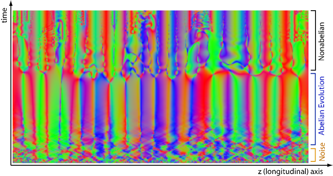
Fig. 1.: Visualization of the spacetime dependence of the color-absolute value of the $x$-component of the induced current obtained from a 1+1-dimensional simulation.

One of the chief obstacles to thermalization in ultrarelativistic heavy-ion collisions is the intrinsic expansion of the matter produced. If the matter expands too quickly then there will not be time enough for its constituents to interact before flying apart into non-interacting particles and therefore the system will not reach thermal equilibrium. In a heavy-ion collision the expansion which is most relevant is the longitudinal expansion of the matter since at early times it’s much larger than the transverse expansion. In the absence of interactions the longitudinal expansion causes the system to quickly become much colder in the longitudinal direction than in the transverse direction, $\langle p_{L}\rangle\ll\langle p_{T}\rangle$. We can then ask how long it would take for interactions to restore isotropy in the $p_{T}$-$p_{L}$ plane. In the bottom-up scenario [1] isotropy is obtained by hard collisions between the high-momentum modes which interact via an isotropically screened gauge interaction. The bottom-up scenario assumed that the underlying soft gauge modes responsible for the screening were the same in an anisotropic plasma as in an isotropic one. In fact, this turns out to be incorrect and in anisotropic plasmas the most important collective mode corresponds to an instability to transverse magnetic field fluctuations [2]. Recent works have shown that the presence of these instabilities is generic for distributions which possess a momentum-space anisotropy [3, 4] and have obtained the full hard-loop action in the presence of an anisotropy [5].

Here I will discuss numerical results obtained within the last year which address the question of the long-time behavior of the instability evolution [6, 7, 8, 9] within the hard-loop framework. This question is non-trivial in QCD due to the presence of non-linear interactions between the gauge degrees of freedom. These non-linear interactions become important when the vector potential amplitudes become $\langle A\rangle_{\rm soft}\sim p_{\rm soft}/g\sim(gp_{\rm hard})/g$, where $p_{\rm hard}$ is the characteristic momentum of the hard particles. In QED there is no such complication and the fields grow exponentially until $\langle A\rangle_{\rm hard}\sim p_{\rm hard}/g$ at which point the hard particles undergo large-angle scattering in the soft background field invalidating the assumptions underpinning the hard-loop effective action. Initial numerical toy models indicated that non-abelian theories in the presence of instabilities would “abelianize” and fields would saturate at $\langle A\rangle_{\rm hard}$ [6]. This picture was largely confirmed by simulations of the full hard-loop gauge dynamics which assumed that the soft gauge fields depended only on the direction parallel to the anisotropy vector and time [7]. However, recent numerical studies have now included the transverse dependence of the gauge field and it seems that the result is then that the gauge field’s dynamics changes its behavior from exponential to linear growth when its amplitude reaches the soft scale, $\langle A\rangle_{\rm soft}\sim p_{\rm hard}$ [8, 9]. This linear growth regime is characterized by a cascade of the energy pumped into the soft scale by the instability to higher momentum plasmon-like modes [10]. Below I will briefly describe the setup which is used by these numerical simulations and then discuss questions which remain in the study of non-abelian plasma instabilities.

In Sec. 4 I will present the method which is used to generate Fig. 1 which shows the spacetime dependence of SU(2) gauge field configurations obtained from a 1+1 dimensional simulation of an anisotropic quark-gluon plasma. Due to the coarseness of our current 3+1-dimensional lattice simulations I will present only visualizations coming from 1d lattice simulations, however, the method is easily adapted to the 3+1-dimensional case.

2 Discretized Hard-Loop Dynamics

At weak gauge coupling $g$, there is a separation of scales in hard momenta $|\mathbf{p}|=p^{0}$ of (ultrarelativistic) plasma constituents, and soft momenta $\sim g|\mathbf{p}|$ pertaining to collective dynamics. The effective field theory for the soft modes that is generated by integrating out the hard plasma modes at one-loop order and in the approximation that the amplitudes of the soft gauge fields obey $A_{\mu}\ll|\mathbf{p}|/g$ is that of gauge-covariant collisionless Boltzmann-Vlasov equations [11]. In equilibrium, the corresponding (nonlocal) effective action is the so-called hard-thermal-loop effective action which has a simple generalization to plasmas with anisotropic momentum distributions [5]. The resulting equations of motion are

$$D_{\nu}(A)F^{\nu\mu} = -g^{2}\int{d^{3}p\over(2\pi)^{3}}{1\over 2|\mathbf{p}|}\,p^{\mu}\,{\partial f(\mathbf{p})\over\partial p^{\beta}}W^{\beta}(x;\mathbf{v})\,,$$

$$F_{\mu\nu}(A)v^{\nu} = \left[v\cdot D(A)\right]W_{\mu}(x;\mathbf{v})\,,$$ (1)

where $f$ is a weighted sum of the quark and gluon distribution functions [5] and $v^{\mu}\equiv p^{\mu}/|\mathbf{p}|=(1,\mathbf{v})$.

At the expense of introducing a continuous set of auxiliary fields $W_{\beta}(x;\mathbf{v})$ the effective field equations are local. These equations of motion are then discretized in spacetime and ${\mathbf{v}}$, and solved numerically in the temporal gauge, $A_{0}=0$. The discretization in ${\mathbf{v}}$-space corresponds to including only a finite set of the auxiliary fields $W_{\beta}(x;\mathbf{v}_{i})$ with $1\leq i\leq N_{W}$. For details on the precise discretizations used see Refs. [8, 9].

3 Numerical Results

During the process of instability growth the soft gauge fields get the energy for their growth from the hard particles. In an abelian plasma this energy grows exponentially until the energy in the soft field is of the same order of magnitude as the energy remaining in the hard particles. As mentioned above in a non-abelian plasma one must rely on numerical simulations due to the presence of strong gauge field self-interactions. Here I will present results for a particle momentum distribution which has been squeezed along the $z$-axis.

3.1 1+1 dimensional simulation

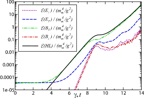
Fig. 2.: Time dependence of energy densities obtained from 1+1-dimensional simulation. Here $\gamma^{*}$ is the growth rate for the dominant unstable mode and $N_{w}=100$, see [7, 9] for details.

In Fig. 2 I have plotted the time dependence of the energy density extracted from the hard particles obtained in a 1+1 dimensional simulation of an anisotropic plasma initialized with very weak random SU(2) color noise [7]. From this Figure we see that after an initial period during which various stable and unstable modes are competing the system enters a period in which the energy density in transverse magnetic fields, ${\cal E}(B_{T})$ (green dot-dot-dashed), grows exponentially with a growth rate of the maximally unstable mode until $\gamma^{*}t\sim 9$. In addition we see that the energy density extracted from the hard particles, ${\cal E}(HL)$ (solid black), also grows exponentially at the same rate during this time indicating that energy extracted from the hard particles primarily goes into producing large amplitude chromo-magnetic fields.

At $\gamma^{*}t\sim 9$ the system enters the “non-linear” regime in which the three- and four-gluon couplings become relevant and there is a brief slowdown in the growth of all quantities shown. However, after some field rearrangement the energy extracted from the particles and the produced soft fields then all grow at approximately the same rate. In this case, the fields would continue to grow until the energy in the soft fields was on the order of the energy in the hard particles, at which time the hard particles would undergo large-angle deflections off the soft fields. This picture, however, only holds in QED or QCD restricted to 1+1 dimensional field configurations (fields are independent of directions transverse to the instability vector). As I will discuss in the next section when the dependence of the chromo-electromagnetic fields on the transverse directions is included the system’s behavior changes dramatically in the non-linear regime. However, in Sec. 4 I will present visualizations which can be produced from these (unrealistic and therefore somewhat academic) 1+1 dimensional simulations.

3.2 3+1 dimensional simulation

As mentioned in the previous section the late-time behavior of the system has a dependence on the dimensionality of the fields assumed in the simulation. In Fig. 3 I have plotted the time dependence of the energy extracted from the hard particles obtained in a 3+1 dimensional simulation of an anisotropic plasma initialized with very weak random color noise [9]. As can be seen from this figure at $m_{\infty}t\sim 60$ there is a change from exponential to linear growth with the late-time linear slope decreasing as $N_{W}$ is increased.

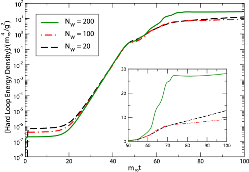
Fig. 3.: Comparison of the energy transferred from hard to soft scales, $\mathcal{E}({\rm HL})$, for 3+1-dimensional simulations with $N_{w}=20,100,200$ on $96^{3},88^{3},69^{3}$ lattices. Inset shows late-time behavior on a linear scale.

The first conclusion that can be drawn from this result is that within non-abelian plasmas instabilities will be less efficient at isotropizing the plasma than in abelian plasmas. However, from a theoretical perspective “saturation” at the soft scale implies that one can still apply the hard-loop effective theory self-consistently to understand the behavior of the system at late times.

4 Visualizations of 1+1 Results

In this section I present visualizations of the gauge-invariant currents generated from our 1+1 dimensional simulation. As mentioned previously, these are merely of academic interest since the 1+1 dimensional simulations do not seem to give the correct late-time behavior for non-abelian gauge groups. However, the visualizations are still interesting in a pedagogical sense and allow one to easily “see” the instabilities in action.

To make these visualizations I use the representation of SU(2) vectors as
$O(3)/Z(2)$ vectors. At each time (vertical axis in Figs. 1, 4, and 5) I loop over the one spatial dimension (horizontal axis), map each SU(2) vector to an O(3) vector, and normalize this vector such that it lies on a unit sphere centered at zero. In order to remove the ambiguity coming from the antipodal equivalence associated with the Z(2) above I then take the absolute value of the vectors obtained from the initial map so that the vectors all map to the positive octant. The vectors in this positive octant of the unit sphere are then mapped directly to RGB colors.

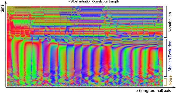
Fig. 4.: Visualization of the spacetime dependence of the color-absolute value of the $x$-component of the induced current obtained from a 1+1-dimensional simulation. Here all color charges have been parallel transported to the leftmost site.

In Fig. 1 I have plotted the spacetime dependence of the $x$-component of the induced current, $j_{x}$, resulting from our 1+1 dimensional simulations with periodic boundary conditions. The bottom-most line in this figure contains the small-amplitude random color initial condition which was used. Proceeding upwards in time the system first goes through a noisy stage in which different unstable and stable modes are competing with the stable left- and right-movers visible as diagonal lines resulting in a ‘criss-cross’ pattern. Next, the system goes through an abelian phase in which the current colors evolve almost independently with a typical spatial wavelength given by the wavelength of the maximally unstable mode [7, 9]. However, once the amplitudes of the color fields reach the non-abelian scale the field self-interactions start to induce ‘splittings’ and the currents begin color-oscillating in time.

Since our simulations are performed in the temporal gauge, $A_{0}=0$, Fig. 1 is the best way to visualize the time-dependence of the gauge field since in this gauge the time-parallel transporter is an identity matrix. However, for assessing the spatial color correlations in the current it is more appropriate to parallel transport the color matrices to a fixed spatial point for comparison. In Fig. 4 I show the result of parallel transporting the same data shown in Fig. 1 to the left-most spatial lattice point ($z=0$). As can be seen, in the abelian phase when the link variables are nearly unity, there is little difference between Figs. 1 and 4; however, as the system approaches the non-abelian phase and the parallel transporters start to differ significantly from unity the two figures are dramatically different. In Fig. 4 at late times, in fact, we can see that local regions where the color is approximately in the same direction emerge. The distance scale over which this occurs is the “abelianization correlation length”. This abelianization correlation length is finite and given approximately by the spatial wavelength of the most unstable mode.

Finally, I include, for comparison, a visualization of the current parallel to the anisotropy vector, $j_{z}$, in Fig. 5.

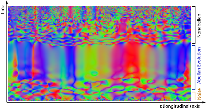
Fig. 5.: Visualization of the spacetime dependence of the color-absolute value of the $z$-component of the induced current obtained from a 1+1-dimensional simulation.

5 Conclusions

The visualizations presented here are mostly novelty but they do allow one to easily see the time evolution of the system and therefore can provide important intuitive information. However, they can provide some insight into the evolution of the system at times prior to when the cascade to higher-momentum modes would set in within the full 3+1-dimensional dynamics. Perhaps, when applied to finer 3+1-dimensional simulations and using surface finding routines they could even be used to better understand the complicated color dynamics occurring at late times.

Looking forward, I note that the latest 3+1-dimensional simulations [8, 9] have only presented results for distributions with a finite ${\mathcal{O}}(1-10)$ anisotropy and these seem to imply that in this case the induced instabilities will not have a significant effect on the hard particles. This means, however, that due to the continued expansion of the system that the anisotropy will increase. It is therefore important to understand the behavior of the system for more extreme anisotropies. Additionally, it would be very interesting to study the hard-loop dynamics in an expanding system. Naively, one expects this to change the growth from $\exp(\tau)$ to $\exp(\sqrt{\tau})$ at short times but there is no clear expectation of what will happen in the linear regime. The short-time picture has been confirmed by early simulations of instability development in an expanding system of classical fields [14]. It would therefore be interesting to incorporate expansion in collisionless Boltzmann-Vlasov transport in the hard-loop regime and study the late-time behavior in this case.

I note in closing that the application of this framework to phenomenologically interesting couplings is suspect since the results obtained strictly only apply at very weak couplings; however, the success of hard-thermal-loop perturbation theory at couplings as large as $g\sim 2$ [11, 12] suggests that the nonequilibrium hard-loop theory might also apply at these large couplings. For going to even larger couplings perhaps colored particle-in-cell simulations [13] could be used if they are extended to include collisions and full 3+1 dynamics.

References

- [1] S. M. H. Wong, Phys. Rev. C54, 2588 (1996); ibid. C56, 1075 (1997). R. Baier, A. H. Mueller, D. Schiff and D. T. Son, Phys. Lett. B 502, 51 (2001); A. H. Mueller, A. I. Shoshi and S. M. H. Wong, arXiv:hep-ph/0505164.
- [2] St. Mrówczyński, Phys. Lett. B 214, 587 (1988); ibid., Phys. Lett. B 314, 118 (1993); ibid., Phys. Rev. C 49, 2191 (1994); ibid., Phys. Lett. B 393, 26 (1997); St. Mrówczyński and M. H. Thoma, Phys. Rev. D 62, 036011 (2000).
- [3] P. Romatschke and M. Strickland, Phys. Rev. D 68, 036004 (2003); ibid., Phys. Rev. D 70, 116006 (2004).
- [4] P. Arnold, J. Lenaghan and G. D. Moore, JHEP 0308, 002 (2003).
- [5] St. Mrówczyński, A. Rebhan and M. Strickland, Phys. Rev. D 70, 025004 (2004).
- [6] P. Arnold and J. Lenaghan, Phys. Rev. D 70, 114007 (2004).
- [7] A. Rebhan, P. Romatschke and M. Strickland, Phys. Rev. Lett. 94, 102303 (2005).
- [8] P. Arnold, G. D. Moore and L. G. Yaffe, Phys. Rev. D 72, 054003 (2005).
- [9] A. Rebhan, P. Romatschke and M. Strickland, JHEP 09, 041 (2005).
- [10] P. Arnold and G. D. Moore, arXiv:hep-ph/0509206; ibid., arXiv:hep-ph/0509226.
- [11] J. P. Blaizot, E. Iancu and A. Rebhan, In R. C. Hwa and X.-N. Wang (eds.): Quark gluon plasma 3, 60-122, arXiv:hep-ph/0303185; U. Kraemmer and A. Rebhan, Rept. Prog. Phys. 67, 351 (2004).
- [12] J. O. Andersen and M. Strickland, Annals Phys. 317, 281 (2005); J. O. Andersen, E. Petitgirard and M. Strickland, Phys. Rev. D 70, 045001 (2004); J. O. Andersen, E. Braaten, E. Petitgirard and M. Strickland, Phys. Rev. D 66, 085016 (2002); J. O. Andersen, E. Braaten and M. Strickland, Phys. Rev. D 61, 074016 (2000); ibid., Phys. Rev. D 61, 014017 (2000); ibid., Phys. Rev. Lett. 83, 2139 (1999).
- [13] A. Dumitru and Y. Nara, Phys. Lett. B 621, 89 (2005).
- [14] P. Romatschke and R. Venugopalan, arXiv:hep-ph/0510121.