Automatized analytic continuation of Mellin-Barnes integrals

Abstract

I describe a package written in MATHEMATICA that automatizes typical operations performed during evaluation of Feynman graphs with Mellin-Barnes (MB) techniques. The main procedure allows to analytically continue a MB integral in a given parameter without any intervention from the user and thus to resolve the singularity structure in this parameter. The package can also perform numerical integrations at specified kinematic points, as long as the integrands have satisfactory convergence properties. I demonstrate that, at least in the case of massive graphs in the physical region, the convergence may turn out to be poor, making naïve numerical integration of MB integrals unusable. I present possible solutions to this problem, but argue that full automatization in such cases may not be achievable.

WUE-ITP-2005-014

PROGRAM SUMMARY

Title of program: MB

Version: 1.1

Catalogue identifier:

Program obtainable from: http://theorie.physik.uni-wuerzburg.de/~mczakon

Computers: All

Operating systems: All

Programming language used: MATHEMATICA, Fortran 77 for numerical evaluation

Memory required to execute with typical data: Sufficient for a typical installation of MATHEMATICA.

No. of bytes in distributed program, including test data: 337900

Distribution format: ASCII

Libraries used: CUBA [1] for numerical evaluation of multidimensional integrals and CERNlib [2] for the implementation of $\Gamma$ and $\psi$ functions in Fortran.

Keywords: Mellin-Barnes integrals, analytic continuation, numerical evaluation, Feynman integrals.

Nature of physical problem: Analytic continuation of Mellin-Barnes integrals in a parameter and subsequent numerical evaluation . This is necessary for evaluation of Feynman integrals from Mellin-Barnes representations.

Method of solution: Recursive accumulation of residue terms occurring when singularities cross integration contours. Numerical integration of multidimensional integrals with the help of the CUBA library.

Restrictions on the complexity of the problem: Limited by the size of the available storage space.

Typical running time: Depending on the problem. Usually seconds for moderate dimensionality integrals.

1 Introduction

The synergy between experiment and theory in the area of elementary particle physics is constantly driving perturbative calculations to higher and higher orders. This is particularly true close to the beginning of the Large Hadron Collider’s operation. Therefore, recent years have seen the emergence of several powerful methods of evaluation of subsequent terms of the perturbative expansion. As far as multiloop Feynman integrals are concerned, the method of differential equations Ref. [3, 4] and Mellin-Barnes integral representations Ref. [5, 6] have proved to be the most successful. Some complicated problems turned out to even require a mixed approach, as advocated, for example, in the case of Bhabha scattering in Ref. [7]. In parallel to analytical approaches, new numeric techniques have been devised, among which the sector decomposition method Ref. [8] occupies a prominent place. Very recently in Ref. [9], the role of Mellin-Barnes integral representations as sources of numeric approximations in the physical region has also been stressed.

In the present work, I will concentrate on Mellin-Barnes integral representations. There are two advantages of this approach. First, it allows for systematic extraction of singularities. Second, the dimensionality of the representation is not directly connected to the number of lines in the graph and therefore, one often arrives at integrals of low dimensionality even for complicated graphs. The calculation of a Feynman integral proceeds in this method in three steps. At first, one derives a representation, then performs the analytic continuation in $\epsilon$, where $d=4-2\epsilon$ is the dimension of spacetime, and finally evaluates the resulting integrals. The first step above can be performed in several different ways, aiming at the simplest possible representation. The various possibilities are described in Ref. [10]. A general algorithm is here only interesting in the case of subsequent numeric integration, see Ref. [9]. The third step cannot be generalized apart from numerical integration, even though some classes of problems can be solved algorithmically, e.g. by reduction to nested sums, see Ref. [11]. It is only in the second step, the analytic continuation, that one can provide an algorithmic solution that would be satisfactory for both analytic and numeric evaluation. This solution is provided by the MATHEMATICA package MB introduced in the present work.

Numeric evaluation of MB integrals has already been mentioned more than once above. Whether just for testing or for the actual calculation, automatization of this step is of value by itself. The package MB can perform the necessary integration by means of FORTRAN, the CUBA library [1] of integration routines, and the CERN library implementation of gamma and psi functions [2]. Since the integrals are infinite range and multidimensional, their feasibility depends strongly on their convergence. In all tested examples, where invariants are in the Euclidean range, the behaviour is exponential and therefore poses no problems. In [9], physical kinematics have also been considered, but the presented examples were restricted to massless graphs exclusively. Here, I notice that massive graphs have worse properties. In fact, I give examples of integrals, which are not even absolutely integrable, and the integral is similar to the Fourier transform of the inverse square root. Such cases can still be treated, but some initial analysis is necessary and it is difficult to see how it could be automatized. Moreover, the techniques will rapidly become inefficient for higher dimensional integrals.

The paper is organized as follows. In the next section, I define the main concepts and present the algorithm for analytic continuation. Subsequently, I describe the package starting with the user interface, low level routines, examples, numerical integration routines and some additional tools. Finally, I briefly summarize and conclude the paper.

2 Analytic continuation of Mellin-Barnes integrals

At the core of the Mellin-Barnes method lies the following representation

$$\frac{1}{(A+B)^{\nu}}=\frac{1}{\Gamma(\nu)}\frac{1}{2\pi i}\int_{-i\infty}^{i\infty}dz\frac{A^{z}}{B^{\nu+z}}\Gamma(-z)\Gamma(\nu+z),$$ (1)

where the contour is chosen in such a way, that the poles of the $\Gamma$ function with $+z$ are separated from the poles of the $\Gamma$ function with $-z$.

This representation can be used in Feynman integral computations in several ways. The easiest is to turn massive propagators into massless and integrate the massless integral, if a formula for general powers of propagators exists. In more complicated cases, one can use some parametric representation of the Feynman integral, which is usually an integral of a product of polynomials raised to some powers, and split the polynomials into pieces that are then integrable by some generalization of the Euler formula

$$\int_{0}^{1}dx\;x^{\alpha-1}(1-x)^{\beta-1}=\frac{\Gamma(\alpha)\Gamma(\beta)}{\Gamma(\alpha+\beta)}.$$ (2)

An extensive discussion of the methods with examples can be found in Ref. [10]. Irrespective of the method, however, the expression for any Feynman integral assumes the form

$$\!\!\!\!\!\!\!\!\!\!\!\!\frac{1}{(2\pi i)^{n}}\int_{-i\infty}^{i\infty}\dots\int_{-i\infty}^{i\infty}\Pi_{i}dz_{i}\;f(z_{1},\dots,z_{n},s_{1},\dots,s_{p},a_{1},\dots,a_{q},\epsilon)\frac{\Pi_{j}\Gamma(A_{j}+V_{j}+c_{j}\epsilon)}{\Pi_{k}\Gamma(B_{k}+W_{k}+d_{k}\epsilon)},$$

(3)

where $s_{i}$ are some kinematic parameters and masses; $a_{i}$ are the powers of the propagators; $A_{i}$, $B_{i}$ are linear combinations of the $a_{i}$; $V_{i}$, $W_{i}$ are linear combinations of $z_{i}$; and $c_{i}$, $d_{i}$ are some numbers. The function $f$ is analytic, in practice a product of powers of the $s_{i}$, with exponents being linear combinations of the remaining parameters.

Because of the assumptions inherent in Eq. (1), the above equation is well defined and corresponds to the original Feynman integral, if the real parts of all of the $\Gamma$ functions have positive arguments. If these conditions cannot be satisfied with $\epsilon=0$, then the integral may develop divergences and analytic continuation to $0$ is necessary to make an expansion in $\epsilon$.

The purpose of the presented package is to perform the analytic continuation of Eq. (3) in $\epsilon$ to some chosen value $\epsilon_{0}$. The algorithm requires to generalize Eq. (3) to allow for $\psi$ functions in the fraction, with $\psi(z)=d\log\Gamma(z)/dz$ and $\psi^{(n)}(z)=d^{n}\psi(z)/dz^{n}$, with the same structure of arguments as those of the $\Gamma$ functions.

2.1 The algorithm

There are two known ways to perform the analytic continuation. The first, introduced in Ref. [5] consists in deforming the integration contours and then shifting them past the poles of the $\Gamma$ functions, which results in residue integrals. It is not clear how to make this method algorithmic, although some attempts in the specific case of massless on-shell double boxes have been undertaken in [12].

The second method, introduced in Ref. [6] assumes fixed contours parallel to the imaginary axis, and the analytic continuation consists in accounting for pole crossings past the contours. As described in Ref. [6], this method is an algorithm. I make one modification with respect to the original, namely I assume that the contours are such that no two contours can be crossed simultaneously. This assumption can always be satisfied by infinitesimal shifts of one of the concerned contours.

It should be clear from the above considerations, that the imaginary parts of the involved variables do not play any role. It is therefore assumed that $z_{i}$, $a_{i}$ and $\epsilon$ are real. With ${\bf z}=(z_{1},\dots,z_{n})$, ${\bf a}=(a_{1},\dots,a_{q})$, and $(I,\epsilon_{I})$ some MB integral with fixed contours and the value of $\epsilon$ fixed at $\epsilon_{I}$, the algorithm can be formalized as in Fig. 1.

Figure 1: Analytic continuation algorithm.

The algorithm has been written for $\Gamma$ functions, but one should add $\psi$ functions, wherever $\Gamma$ functions occur. Upon termination, the set $C$ contains all the integrals following from the analytic continuation. It should be clear that it is the “if” clause that does not allow for crossings of two different contours at a time.

A comment about the choice of the contours is in order. Even though all the choices are equivalent, one would like to have the smallest possible number of contributions. An improvement implemented in the package is to first gather all the residue points, and then try to add additional constraints on the contours such that these residues would not occur. If some subset of these constraints can be satisfied, then the number of residues will be reduced. This is not an algorithm that leads to an absolute minimum of the number of residues, it gives, however, at least some reduction of the number of contributions.

Finally, one should notice that the technique of Ref. [6] has been similarly formalized in Ref. [9].

3 The package

3.1 User interface

The main routine performing the analytic continuation is

MBcontinue[integrand, limit, {fixedVarRules, intVarRules}, options]

where the input arguments are

• integrand: any object accepted by MATHEMATICA. Notice that the singularities are determined by analyzing $\Gamma$ and $\psi$ functions only.

• limit: a rule, x -> x0, which specifies at the same time the variable, x, in which the analytic continuation is performed and the point, x0, which the user wants to reach.

• fixedVarRules: a list of rules giving the values of the real parts of the variables, which are not integrated over. In particular, it must contain the starting value of the variable, in which the analytic continuation is performed.

• intVarRules: a list of rules giving the real parts of the integration variables.

• options:

  • Level: an integer specifying the level at which the recursive analytic continuation will be stopped. By default, it is set to infinity.

  • Skeleton: a boolean value. If True, the residues will be identified, but not calculated. This is achieved by replacing all $\Gamma$ and $\psi$ functions by a dummy function MBgam. The purpose of this option is to quickly determine the total number of integrals. By default this option is set to False.

  • Residues: a boolean value. If True, the output will also contain the list of Residue points besides the actual values of the residues. This is mainly for internal use and is set by default to False.

  • Verbose: a boolean value. If True, the level is printed as well as the position on the list of the currently continued integral and the residue points together with the signs of the residues. This option is switched on by default.

The output is a nested list obtained by replacing, at every level, the integral to be continued by its residues and the original integral at the limit. The elements are

MBint[integrand, {fixedVarRules, intVarRules}]

objects, where the integrand can be expanded around the limit, which is placed on the fixedVarRules list. If the user specified a finite level, then there might also occur

MBitc[integrand, limit, {fixedVarRules, intVarRules}, Options]

objects, where “itc” stands for “integral to continue”. These are not yet regular at the limit and require further recursive analytic continuation. Furthermore, if the user set the Residues option to True, there will also be a list of

MBres[sign, var, val],

objects, which signal that there was a residue taken in the variable, var, at the value, val, with sign.

Restricted input checking has been implemented, and as long as the input is syntactically correct, the only error that may occur is (see Section 2.1 for further details)

contour starts and/or ends on a pole of Gamma[z]

In this case the procedure stops and gives an inequality for an integration variable that is sufficient to remove the problem.

The integration contours are found with

MBoptimizedRules[integrand, limit, constraints, fixedVars, options]

For a description of the integrand and limit see MBcontinue. The remaining input parameters are as follows

• constraints: a list of additional constraints (inequalities) specified by the user. This should usually be left empty, but might be used for experimentation in order to search for contours that might possibly give less residues.

• fixedVars: a list of variables, which should be considered fixed during analytic continuation. The integration variables are determined automatically from the arguments of the $\Gamma$ and $\psi$ functions.

• options:

  • Level: specifies the level up to which optimization of the contours will be performed. This option should only be used for very large calculations. Since in this case, the contours are only partially tested, the user will have to correct them himself, if poles lying on a contour are encountered. In practice, independent, small shifts should be sufficient for this purpose.

The output matches precisely the form needed in the input of MBcontinue, i.e.

{fixedVarRules, intVarRules}

Notice that this procedure not only reduces the number of residues, but also generates such contours that, during analytic continuation, no contours will start or end on a pole.

During the determination of the real parts, warning messages are generated. These can be ignored apart from the case when there is a single message

no rules could be found to regulate this integral

and the output is an empty list. In this case, the integral cannot be regulated and the user has to provide another one, e.g. by introducing a further regulator parameter, for example a propagator power, and performing two subsequent analytic continuations.

Once the integrals are determined, they can be either merged, i.e. those that have the same contour will be added by linearity; preselected, i.e. those that would vanish in a given order of expansion in some parameter are rejected; or expanded. These tasks are achieved with the following utilities.

MBmerge[integrals]

Merges MBint objects on the integrals list by linearity, if they have the same contours. Vanishing integrals are rejected.

MBpreselect[integrals, {x, x0, n}]

Rejects those MBint objects on the integrals list that would vanish after expansion in the variable x, around the point x0, up to order n.

MBexpand[integrals, norm, {x, x0, n}]

Expands MBint objects on the integrals list around the point x0, in the variable x, up to order n. A normalization factor, norm, is included in every integrand.

3.2 Low level routines

The routines described in the previous section form the interface. It might happen that the user would like to use the low level routines, which actually perform the calculation.

MBresidues[integrand, limit, {fixedVarRules, intVarRules}, options]

Performs a single step in the recursive analytic continuation algorithm, i.e. it finds all the residues for a given integral, but does not proceed with the analytic continuation of the resulting integrals. All the arguments and options are the same as in MBcontinue, apart from Level, which is in this case meaningless.

MBrules[integrand, constraints, fixedVars]

Finds the real parts of all the fixed and integration variables, such that the real parts of the arguments of all the $\Gamma$ and $\psi$ functions be positive. The difference to MBoptimizedRules is that no attempt is made to optimize the number of residues or even check whether the contours will not lead to problems with MBcontinue. To perform these tests, MBoptimizedRules needs the limit of the continuation, which is left unspecified here. This routine is of particular interest, because one may use it to write another contour optimization algorithm.

MBrules[integrand, limit, constraints, fixedVars]

Same as MBrules, but check the contours, so that a complete analytic continuation with MBcontinue can be performed.

3.3 Examples

Figure 2: The $B_{0}(s,ms,ms)$ function, with $s=p^{2}$ and $ms=m^{2}$.

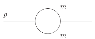
As a first example, I consider the $B_{0}$ function with two equal masses, Fig. 2. After introduction of two MB integrations (the integral can be further simplified by the use of the first Barnes lemma, see Section 3.5) and normalization of the integration measure with $1/(i\pi^{d/2})$, the expression reads

In[1]:= int = b0[s, 1+z1, 1+z2]*ms^z1*ms^z2*
        Gamma[-z1]*Gamma[1+z1]*Gamma[-z2]*Gamma[1+z2] /. z1 -> z1-z2

Out[1]:= (m1s^z1*(-s)^(-ep - z1)*Gamma[ep + z1]*Gamma[1 - ep - z2]*
         Gamma[-z2]*Gamma[-z1 + z2]*Gamma[1 - ep - z1 + z2])/ Gamma[2
         - 2*ep - z1]
    

The user must now determine the contours, or more precisely, the real parts of the contours.

In[2]:= rules = MBoptimizedRules[int, ep -> 0, {}, {ep}]

MBrules::norules: no rules could be found to regulate this integral

MBrules::norules: no rules could be found to regulate this integral

Out[2]:= {{ep -> 7/8}, {z1 -> -3/4, z2 -> -1/2}}
    

As explained above, the two warning messages have been generated during the determination of the contours, and since some real parts have been found, they are harmless.

The user can now perform the analytic continuation

In[3]:= cont = MBcontinue[int, ep -> 0, rules]

Level 1

Taking +residue in z1 = -ep

Level 2

Integral {1}

Taking +residue in z2 = -ep

Level 3

Integral {1, 1}

3 integral(s) found

Out[3]:= {{{MBint[(Gamma[1 - ep]*Gamma[ep])/ (m1s^ep*Gamma[2 - ep]),
              {{ep -> 0}, {}}]},  MBint[(Gamma[1 - ep -
              z2]*Gamma[-z2]*Gamma[1 + z2]* Gamma[ep +
              z2])/(m1s^ep*Gamma[2 - ep]),  {{ep -> 0}, {z2 ->
              -1/2}}]},  MBint[(m1s^z1*(-s)^(-ep - z1)*Gamma[ep + z1]*
              Gamma[1 - ep - z2]*Gamma[-z2]*Gamma[-z1 + z2]* Gamma[1 -
              ep - z1 + z2])/Gamma[2 - 2*ep - z1],  {{ep -> 0}, {z1 ->
              -3/4, z2 -> -1/2}}]}
    

At this stage, the user can, for example, expand the integrals to determine the divergence

In[4]:= div = MBexpand[cont, Exp[ep EulerGamma], {ep, 0, -1}]

Out[4]:= {{{MBint[ep^(-1), {{ep -> 0}, {}}]}}}
    

This is the well known value for the $B_{0}$ function. The integral header, MBint, is kept, because in general, even the divergences may be given by nontrivial MB integrals.

Figure 3: First planar QED box master integral, B1. The wavy lines are massless, whereas the continuous are massive and on-shell.

Figure 4: Second planar QED box master integral, B2. The notation is the same as in Fig. 3.

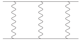
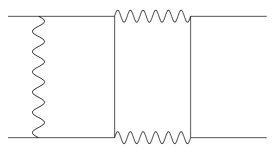
Together with the MB.m package, two example notebooks are provided. The first one, MBexamples1.nb, contains massive box integrals, in particular, the first and the second planar 7-line QED box master integrals, Fig. 3 and Fig. 4 respectively. It is found that in the first case, only 5 integrals contribute to the finite part, which is less than has been determined in Ref. [13] by another method of analytic continuation. After merging, both integrals have just 4 contributions. I have checked by numerical integration that the results agree with Ref. [13] and Ref. [14].

Figure 5: The B5l3md2 integral. The notation is the same as in Fig. 3.

Figure 6: A regularized version of the B5l3md2 integral. A finite result can be derived from the general representation for B2, when $a_{6}\rightarrow 0$.

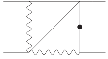
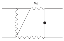
An interesting example is the B5l3md2 integral, Fig. 5, from Ref. [15]. If one uses the general representation from Ref. [14], and simply sets the powers of the propagators to appropriate values, then the integral seems to vanish, due to a $\Gamma$ function in the denominator, $1/\Gamma(0)=0$. To overcome this problem, one keeps one of the powers as a parameter, as in Fig. 6 and does first an analytic continuation in this parameter. In this way, one obtains the following MB representation

$$\!\!\!\!\!\!\!\!\!\!\!\!\!\!\!\frac{1}{(2\pi i)^{4}}\frac{1}{\Gamma(-2\epsilon)}\int_{-i\infty}^{i\infty}\int_{-i\infty}^{i\infty}\int_{-i\infty}^{i\infty}\int_{-i\infty}^{i\infty}\;\;dz_{1}\;dz_{2}\;dz_{5}\;dz_{6}\;(-s)^{-2-2\epsilon-z_{5}-z_{6}}\left(\frac{t}{s}\right)^{z_{1}}$$

$$\times \frac{\Gamma(-z_{1})\Gamma(1+z_{1})\Gamma(-1-2\epsilon-z_{2})\Gamma(1+z_{2})\Gamma(-3-4\epsilon-2z_{1}-z_{2}-2z_{5})}{\Gamma(-1-2\epsilon-z_{2}-2z_{5})\Gamma(-3\epsilon-z_{5})\Gamma(-3-4\epsilon-2z_{1}-z_{2}-2z_{5}-2z_{6})}$$

$$\times \Gamma(-1-\epsilon-z_{5})\Gamma(-\epsilon-z_{2}-z_{5})\Gamma(-z_{5})\Gamma(2+\epsilon+z_{1}+z_{2}+z_{5})$$

$$\times \Gamma(-1-2\epsilon-z_{1}-z_{5}-z_{6})\Gamma(-2-2\epsilon-z_{1}-z_{2}-z_{5}-z_{6})\Gamma(-z_{6})$$

$$\times \Gamma(2+2\epsilon+z_{1}+z_{5}+z_{6}).$$

The presence of the $1/\Gamma(-2\epsilon)$ factor means that as long as we are only interested in the finite part, the integral is just threefold. This is, of course, confirmed by explicit continuation as can be checked in MBexamples1.nb, where three contributions are obtained. This result has been numerically checked against the one obtained by the sector decomposition method.

Figure 7: Massless on-shell non-planar double box integral, NP.

Figure 8: Massless on-shell triple box integral, T.

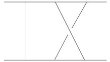
The second notebook, MBexamples2.nb, contains two massless on-shell box integrals, the two-loop non-planar NP, Fig. 7, and the three-loop planar T, Fig. 8. In the first case, I evaluate the first three poles of the expansion and obtain at the symmetric point, $s=-1,t=-1,u=-1$

$$\mbox{NP}=\Gamma(3+2\epsilon)\left(\frac{7}{4\epsilon^{4}}-\frac{3}{\epsilon^{3}}-\frac{1}{\epsilon^{2}}\left(\frac{7}{2}+\frac{47\pi^{2}}{24}\right)+\dots\right),$$ (4)

in perfect agreement with Ref. [6]. Similarly, I recover the value of the first three poles of the triple-box integral Ref. [16]

$$\mbox{T}=-\frac{e^{-3\epsilon\gamma_{E}}}{s^{3}(-t)^{1+3\epsilon}}\left(\frac{16}{9\epsilon^{6}}-\frac{5\log(s/t)}{3\epsilon^{5}}-\frac{3\pi^{2}}{2\epsilon^{4}}+\dots\right).$$ (5)

In both cases the lowest order pole was given by one-dimensional integrals that could be made with the first Barnes lemma, see Section 3.5.

3.4 Numerical integration

There are two factors determining the rate of convergence of MB integrals Eq. (3): the behaviour of the product of gamma functions for large imaginary arguments and the behaviour of the analytic $f$ function.

In the limit of large imaginary argument, the $\Gamma$ function exhibits an oscillatory behaviour, an exponential damping factor and a power law. Indeed, for $a,b\in{\rm I\mkern-3.0muR}$ and $b\gg 0$

$$\Gamma(a+ib) \simeq \sqrt{2\pi}\;e^{i\frac{\pi}{4}(2a-1)}\;e^{ib\;(\log{b}-1)}\;e^{-\frac{b\pi}{2}}\;b^{a-1/2},$$ (6)

$$\Gamma(a-ib) \simeq \sqrt{2\pi}\;e^{-i\frac{\pi}{4}(2a-1)}\;e^{-ib\;(\log{b}-1)}\;e^{-\frac{b\pi}{2}}\;b^{a-1/2}.$$ (7)

If we combine different gamma functions the exponential factor might in principle disappear, but fortunately in all cases studied it did not.

On the other hand, as explained in Ref. [10], the $f$ function is usually a product of terms of the form

$$(-s)^{-z},$$ (8)

where $s$ is some kinematic invariant (e.g. a Mandelstam variable) and $z$ is one of the integration variables. As long, as we are in the Euclidean regime, i.e. $s<0$, Eq. (8) contributes another oscillatory factor and cannot influence the convergence of the integral. For positive values, however, we will have

$$(-s)^{-z}=e^{-z\log(-s)}=e^{-z(\log(s)-i\pi)}=e^{ia\pi}\;s^{z}\;e^{b\pi},$$ (9)

where $z=a-ib$. It is clear, that the exponential factor can compensate the damping from the product of gamma functions.

An interesting example, which illustrates the problem is provided by the leading pole term of the first planar 7-line QED box integral, Fig. 3, which is given by

$$-\frac{e^{-2\epsilon\gamma_{E}}}{2s^{2}(-t)^{1+2\epsilon}}\frac{1}{\epsilon^{2}}\frac{1}{(2\pi i)^{2}} \!\!\!\!\!\!\!\int_{-i\infty}^{i\infty}\int_{-i\infty}^{i\infty}dz_{1}\;dz_{2}\;(-s)^{-z_{1}-z_{2}}$$ (10)

$$\times \frac{\Gamma^{3}(-z_{1})\Gamma(1+z_{1})\Gamma^{3}(-z_{2})\Gamma(1+z_{2})}{\Gamma(-2z_{1})\Gamma(-2z_{2})},$$

where $\Re\;z_{1}=\Re\;z_{2}=-1/2$. This is just a product of two one-dimensional integrals, which can be done by closing contours and resumming the residues, with the result

$$\frac{1}{2\pi i}\int_{-i\infty}^{i\infty}dz_{1}\;(-s)^{-z_{1}}\frac{\Gamma^{3}(-z_{1})\Gamma(1+z_{1})}{\Gamma(-2z_{1})}=-\frac{4}{\sqrt{\frac{4}{s}-1}}\arcsin\sqrt{\frac{s}{4}},$$ (11)

below threshold, i.e. for $0\leq s\leq 4$. For $z_{1}=-1/2-ib$, $b\gg 0$, the integrand behaves as

$$-\frac{1+i}{\sqrt{2}}\;\sqrt{\pi s}\;\frac{e^{i\log{(s/4)}\;b}}{\sqrt{b}}.$$ (12)

As anticipated, the exponential factor disappeared. Worse even, the integrand is not absolutely integrable. It is interesting to note, that the frequency of the oscillation, $\log{(s/4)}$, encodes the threshold. Further examples seem to confirm that this is a general property. Fortunately, this integral can be evaluated using standard techniques for infinite range oscillatory integrands. With the Pantis’ method [17]

$$\int_{-\infty}^{\infty}db\;e^{-i\omega b}f(b)\simeq\int_{-b_{0}}^{\infty}db\;e^{-i\omega b}f(b)+\frac{1}{i\omega}e^{i\omega b_{0}}f(-b_{0}),$$ (13)

setting $s=2$ and $b_{0}=40$ the value of the integral in Eq. (11) is $\simeq-3.17-0.09i$, to be compared to the exact result, which is $-\pi$.

One would be tempted to assume that the slowly convergent oscillatory behaviour can be factorized in one integration variable and that the remaining integrations are fast convergent. This assumption is false, as shown in Fig. (9), which represents the integrand in $z_{1}$ of the original integral after shifting $z_{1}\rightarrow z_{1}-z_{2}$ and up to normalization factors

$$\frac{1}{(2\pi i)^{2}}(-s)^{-z_{1}}\int_{-i\infty}^{i\infty}dz_{2}\;\frac{\Gamma^{3}(-z_{1}+z_{2})\Gamma(1+z_{1}-z_{2})\Gamma^{3}(-z_{2})\Gamma(1+z_{2})}{\Gamma(-2z_{1}+2z_{2})\Gamma(-2z_{2})}.$$ (14)

Apparently, this does not seem to be integrable at all, and certainly no numerical method would provide a reasonable estimate, even if it would be integrable.

Figure 9: Real part of the integral Eq. (14) at s = 2.

In conclusion, one encounters massive Feynman integrals, which require, in the physical regime, multidimensional integration of slowly convergent oscillatory functions over infinite range. This problem can be solved, but the efficiency of the methods is very low and acceptable only for low dimensions. Furthermore, it might be necessary to shift the integration variables to obtain convergent representations. The latter task is certainly very difficult to automatize.

The above discussion does not change anything to the fact that MB integrals provide reliable numerics in the Euclidean regime for all encountered integrals and in the Minkowski regime for the massless ones. It is of course not excluded that some massive integrals can also be done reliably without special methods, but this has to be checked in specific cases.

The MB package provides routines that can perform numerical integrations of MB representations. In order to work, the libraries libcuba.a from CUBA [1], libkernlib.a and libmathlib.a from CERNlib [2] have to be installed either in the working directory or in a globally accessible directory with libraries, and the Fortran compiler has to be called f77. In case, the user wanted to change these defaults, it would be necessary to change the internal code of MB.m.

The main routine for numerical integration is

MBintegrate[integrals, kinematics, options]

where the input arguments are

• integrals: a list of integrals as provided by MBexpand.

• kinematics: a list of rules providing numeric values for all the parameters (usually kinematic invariants) besides the expansion variable and the integration variables. If the user is interested in Minkowski kinematics then a small imaginary part should be added. Even though this is just an approximation, it is justified by the fact, that the final result has usually much lower precision than the error introduced by such a procedure.

• options:

  • NamePrefix: by default the Fortran programs generated for integrals in more than one variable are called MBpart1x0, etc. where the last number is the power of the expansion variable x and part1 denotes the first integral at this order. With this option one can change the prefix MB.

  • PrecisionGoal, AccuracyGoal, MaxPoints, MaxRecursion: numerical integration options as in NIntegrate. The defaults are respectively $4$, $12$, $10^{6}$, $10^{3}$, and have been tuned to several problems solved with the package.

  • MaxCuhreDim: dimension threshold, 4 by default, above which Vegas will be used for the evaluation of the integrals instead of Cuhre.

  • Complex: by default, only the real part of the integrals is evaluated, with this option set to True, the imaginary part will also be given.

  • FixedContours: contours will not be shifted if this option is set to True. For a detailed explanation, see MBshiftContours below.

  • NoHigherDimensional: by default, the complete integration is performed within MBintegrate, however with this option set to True, 1-dimensional integrals are evaluated and the Fortran programs are prepared, but not run. This may be used to run them in parallel for example.

  • Debug: with this option set to True, the Fortran programs are kept after evaluation and the value of every integral is given within MBval[value, error, probability, part] objects, where value, error and probability are given by CUBA, and part is the number of the integral. This provides a primitive means of improving the calculation by tuning only specific integrals, since the integration parameters can be easily changed in the Fortran programs.

  • Verbose: by default the progress of the integration is printed to the screen. This can be switched off by setting this option to False.

Instead of providing a detailed description of the output, I illustrate MBintegrate on the example of the “tennis court integral”, Fig. (10), introduced and calculated analytically in [18]. Since, it has never been confirmed independently, this example supports the correctness of the analytical result.

Figure 10: Tennis court integral, $I_{4}^{(3)b}$, containing a factor of $(p+r)^{2}$.

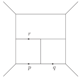
Similarly as in [18], a factor of $-(-s)^{-1-3\epsilon}t^{-2}$ has been taken out. If expanded is the result provided by MBexpand, which contains 65 integrals, then the numerical evaluation proceeds as follows

In[3] := MBintegrate[expanded, {s -> -2, t -> -3}]

Shifting contours...

Performing 30 1-dimensional integrations...1...2...3...4...5...6...
7...8...9...10...11...12...13...14...15...16...17...18...19...20...
21...22...23...24...25...26...27...28...29...30

Higher-dimensional integrals

Preparing MBpart1ep0 (dim 6)

Preparing MBpart2ep0 (dim 6)
.
.
.
Preparing MBpart58ep-1 (dim 4)
.
.
.
Running MBpart1ep0

Running MBpart2ep0
.
.
.
{154.50857084232496 + 1.7777777777777777/ep^6 -
  0.8785077342343561/ep^5 - 15.544672574293408/ep^4 -
  20.903348302858618/ep^3 + 20.868443575404378/ep^2 +
  84.4035478542778/ep,
 {1.454748334713152 + 0.0012476956259284788/ep^3 +
   0.01736836792954924/ep^2 + 0.3243732528120632/ep, 0}}
    

At a first stage, the contours are shifted with MBshiftContours, then the 1-dimensional integrals are evaluated in MATHEMATICA. Subsequently, Fortran programs for the higher dimensional integrals are prepared and run. The user can easily see the names of the programs and the dimensions of the integrals. Finally, the result is given in the form of a list. The first element is the result itself, whereas the second element is a sublist giving the errors on the real and imaginary parts respectively. It is important to note, that the errors are estimated from the square root of the sum of the squares of the errors of each of the higher dimensional integrals. Therefore, in the example above, the errors start at $1/\epsilon^{3}$, because up to this pole, there were only 1-dimensional integrals. This also implies that it is assumed that the error from the 1-dimensional integrals is negligible. The above calculation took about 1 hour on a 2.4 GHz notebook, with a claimed error on the finite part of about 1% ($1.4$ against $154.5$ above). If compared to the exact result

$$\!\!\!\!\frac{1.77778}{\epsilon^{6}}-\frac{0.878508}{\epsilon^{5}}-\frac{15.5447}{\epsilon^{4}}-\frac{20.9033}{\epsilon^{3}}+\frac{20.8679}{\epsilon^{2}}+\frac{84.4068}{\epsilon}+154.379,$$

the error is rather at the permille level. Further numerical evaluation examples can be found in the two notebooks provided with the package.

A utility related to numerical integration, which is of interest by itself is

MBshiftContours[integrals]

where the only argument is a list of integrals as provided by MBexpand. The idea here, is that if there is a contour passing between two poles of a $\Gamma$ function, then the further it will stay from both of them, the less peaked will the integrand be. Since the contours have more or less random distances to the poles, it is wise to shift them before numerics to improve stability. This is achieved by the above utility.

3.5 Additional tools

Apart from performing the analytic continuation of a MB integral, one is usually interested in simplifying the integrals as much as possible. This is of utmost importance, if one is interested in obtaining analytic results. It is often the case, that some of the integrations can be performed exactly with the help of Barnes’ lemmas.

1st Barnes’ lemma

$$\int_{-i\infty}^{i\infty} dz \Gamma(a+z)\Gamma(b+z)\Gamma(c-z)\Gamma(d-z)=$$ (16)

$$\frac{\Gamma(a+c)\Gamma(a+d)\Gamma(b+c)\Gamma(b+d)}{\Gamma(a+b+c+d)}.$$

2nd Barnes’ lemma

$$\int_{-i\infty}^{i\infty} dz \;\frac{\Gamma(a+z)\Gamma(b+z)\Gamma(c+z)\Gamma(d-z)\Gamma(e-z)}{\Gamma(a+b+c+d+e+z)}=$$ (17)

$$\frac{\Gamma(a+d)\Gamma(a+e)\Gamma(b+d)\Gamma(b+e)\Gamma(c+d)\Gamma(c+e)}{\Gamma(a+b+d+e)\Gamma(a+c+d+e)\Gamma(b+c+d+e)}.$$

Both of them are valid only if the integration contour is such that the poles corresponding to $\Gamma$’s with positive $z$ are separated from the poles with negative $z$. If this is the case, the user can apply the rules defined as

barnes1[z] and barnes2[z],

where z is the integration variable. An example is the simplification of the integral for the $B_{0}$ function

In[1]:= int = b0[s, 1 + z1, 1 + z2]*ms^z1*ms^z2* Gamma[-z1]*Gamma[1 +
        z1]*Gamma[-z2]*Gamma[1 + z2] /.  z1 -> z1 - z2 /. barnes1[z2]

Out[1]:= (ms^z1*(-s)^(-ep - z1)*Gamma[1 - ep - z1]^2*Gamma[-z1]*
         Gamma[ep + z1])/Gamma[2 - 2*ep - 2*z1]
    

This is, however, a rare situation. Most of the time, the Barnes’ lemmas are applicable to integrals after analytic continuation and expansion. In this case, the procedure generates integrals with contours parallel to the imaginary axis and the contour might not separate the poles of the $\Gamma$ functions. In such cases one uses various corollaries to the lemmas, see e.g. Ref. [5].

Figure 11: Regularization of the integrals in the Barnes lemmas by shifting the poles, in such a way that the contour separates the poles.

I propose here an automatic procedure based on MBcontinue. The idea is to shift all of the $a,b,...$ variables by $\epsilon$, such that the contours be separated and then analytically continue with $\epsilon$ to $0$, as illustrated in Fig. 11. In the case of the first Barnes lemma, the shift is determined by the condition

$$\epsilon>\max\left(-\min(a,b)-\Re(z),\;\Re(z)-\min(c,d)\right).$$ (18)

This algorithm is implemented in the following two routines:

Barnes1[MBint[integrand,{fixedVarRules,intVarRules}],z]

and

Barnes2[MBint[integrand,{fixedVarRules,intVarRules}],z]

The arguments are as described in MBcontinue and z is the integration variable that should be eliminated by Barnes’ lemma. An example usage can be found in MBexamples2.nb.

In the case, where the integral contains a $\psi$ function, the user has to apply the lemma to the corresponding integrand with a $\Gamma$ function and only then derive the result. This might be automatized in the future.

Of lesser importance are the remaining tools. To help in the construction of efficient MB integrals, there are several known exact expressions for the $A_{0}$, $B_{0}$ and $C_{0}$ functions taken from the Appendix of Ref. [10]. Details can be found directly in the code of MB.m. In case the user would like to construct his representation directly from a Feynman parameter integral as is done e.g. in Ref. [6], there is also a routine

FUPolynomials[integrand, momenta, invariants]

that generates the $F$ and $U$ polynomials in the notation of Ref. [8]. The input is

• integrand: a product of propagators DS[k,m,n] = $1/(k^{2}-m^{2})^{n}$.

• momenta: the loop momenta.

• invariants: a list of rules, e.g. p1*p2 -> 1/2*s-m^2, which transform products of external momenta into some suitable notation, for example the Mandelstam variables.

In the output, one obtains a list of four elements. First come the $F$ and $U$ polynomials, then the $M$ matrix and $Q$ vector again in the notation of Ref. [8].

4 Conclusions

I presented a practical tool for automatic analytic continuation of MB integrals. It can be used either as part of a Feynman diagram calculation leading to an analytic result in terms of some known functions, or as a tool for directly providing numerical results. Irrespective of the aim, the most cumbersome part of the MB technique has been reduced to a mere use of one MATHEMATICA function, making high order calculations in perturbation theory significantly easier and more accessible to the interested.

References

- [1] T. Hahn, Comput. Phys. Commun. 168 (2005) 78.
- [2] CERN Program Library, obtainable from http://cernlib.web.cern.ch/cernlib/
- [3] A. V. Kotikov, Phys. Lett. B 267 (1991) 123.
- [4] E. Remiddi, Nuovo Cim. A 110 (1997) 1435.
- [5] V. A. Smirnov, Phys. Lett. B 460 (1999) 397.
- [6] J. B. Tausk, Phys. Lett. B 469 (1999) 225.
- [7] M. Czakon, J. Gluza and T. Riemann, arXiv:hep-ph/0511187.
- [8] T. Binoth and G. Heinrich, Nucl. Phys. B 585 (2000) 741.
- [9] C. Anastasiou and A. Daleo, arXiv:hep-ph/0511176.
- [10] V. A. Smirnov, “Evaluating Feynman integrals”, Springer (Berlin, Germany) 2002.
- [11] J. A. M. Vermaseren, Int. J. Mod. Phys. A 14 (1999) 2037, S. Moch, P. Uwer and S. Weinzierl, J. Math. Phys. 43 (2002) 3363; S. Moch and P. Uwer, arXiv:math-ph/0508008.
- [12] V. A. Smirnov and O. L. Veretin, Nucl. Phys. B 566 (2000) 469.
- [13] V. A. Smirnov, Phys. Lett. B 524 (2002) 129.
- [14] G. Heinrich and V. A. Smirnov, Phys. Lett. B 598 (2004) 55.
- [15] M. Czakon, J. Gluza and T. Riemann, Nucl. Phys. Proc. Suppl. 135 (2004) 83; M. Czakon, J. Gluza and T. Riemann, Phys. Rev. D 71 (2005) 073009.
- [16] V. A. Smirnov, Phys. Lett. B 567 (2003) 193.
- [17] P. K. Kythe, M. R. Schäferkotter, “Computational Methods for Integration”, Chapman & Hall/CRC, 2005.
- [18] Z. Bern, L. J. Dixon and V. A. Smirnov, Phys. Rev. D 72 (2005) 085001