Impact of the higher twist effects on the $\gamma\gamma^{*}\to\pi^{0}$ transition form factor

Abstract

We reanalize the $\gamma\gamma^{*}\to\pi^{0}$ transition form factor $F_{\pi\gamma}(Q^{2})$ within the QCD light-cone sum rules method with the twist-4 accuracy. In computations, the pion leading twist distribution amplitude (DA) with two nonasymptotic terms and the renormalon method-inspired twist-4 DAs are used. The latters allow us to estimate impact of effects due to higher conformal spin components in the pion twist-4 DAs on the form factor $F_{\pi\gamma}(Q^{2})$. Obtained theoretical predictions are employed to deduce constraints on the pion DAs from CELLO and CLEO data.

I Introduction

The form factor (FF) $F_{\pi\gamma}(Q^{2})$ of the electromagnetic transition $\gamma\gamma^{*}\to\pi^{0}$ is one of the simplest exclusive processes, for investigation of which at large momentum transfers methods of the perturbative QCD (PQCD) can be applied LB80 ; ER80 ; DM80 . For computation of $F_{\pi\gamma}(Q^{2})$ various theoretical methods and schemes were proposed. They range from the PQCD calculations LB80 ; ABR83 , the light-cone sum rules (LCSR) Kd99 ; SY00 ; BMS03 , to the running coupling approach A01 , employed to estimate power-suppressed corrections to $F_{\pi\gamma}(Q^{2})$. All of these methods are based on the PQCD factorization theorems, in accordance of which the amplitude of an exclusive process can be computed as the convolution integral of a hard-scattering amplitude and the process-independent distribution amplitude (DA) of an involved into the process hadron(s). The hard-scattering amplitude is calculable within the QCD perturbation theory, whereas the hadron (in our case, the pion) DAs are universal functions containing nonperturbative information on hadronic binding effects, and cannot be obtained using tools of PQCD. Hence, the hadron DAs emerge as one of the two building blocks in studying numerous exclusive processes.

To calculate the $\gamma\gamma^{*}\to\pi^{0}$ transition FF in the framework of the QCD LCSR method Kd99 , adopted also in this paper, the knowledge of the pion different twist DAs $\varphi_{\pi}^{(t)}(u,\mu_{F}^{2})$ is required. As we have just mentioned, they cannot be found by means of PQCD. Their factorization scale $\mu_{F}^{2}$ dependence is governed by PQCD, but an input information at the starting point of evolution, i.e., the dependence of the DAs on the variable $u$ (the longitudinal momentum fraction carried by the quark in the pion) at the normalization point $\mu_{0}^{2}$, has to be extracted from experimental data or derived via nonperturbative methods, for example, the QCD sum rules CZ84 , instanton-based models Dor , or lattice simulations Lattice . Nevertheless, there exists the regular theoretical approach for treatment of the hadron DAs. It suggests the parametrization of the hadron DAs in terms of a partial wave expansion in conformal spin, and rely on the conformal symmetry of the QCD Lagrangian BKM03 . It is important that any parametrization of DA based on a truncated conformal expansion is consistent with the QCD equations of motion BF90 and is preserved by the QCD evolution to the leading logarithmic accuracy ER80 ; LB80 . Therefore, the conformal expansion provides a practical framework for modeling of the hadron DAs BF90 ; BB98 and is widely used for investigation of numerous exclusive processes in QCD.

Because of the increasing number of parameters at higher conformal spins and practical difficulties in phenomenological applications, one has to restrict one’s self by taking into account only the first few terms in the conformal expansion of DAs. As a result, the contributions of higher conformal spins to DAs in the existing calculations are neglected. At the same time, the suppression of higher spin contributions and the convergence of conformal expansion at present experimentally accessible energy regimes is not obvious and requires further studies.

The renormalon model proposed in Refs. An00 ; BGG04 pursues to test precisely this issue; that is, to set a plausible upper bound for the possible contributions of higher conformal spins that so far escaped attention. The renormalon approach employs the assumption that the infrared renormalon ambiguities in the leading twist coefficient functions should cancel the ultraviolet renormalon ambiguities in the matrix elements of twist-4 operators in a relevant operator product expansion. Such cancellation was proved by explicit calculations in the case of the simple exclusive amplitude involving pseudoscalar and vector mesons BGG04 . The idea of the renormalon model for the meson twist-4 DAs is to define them by taking the functional form of the corresponding ultraviolet renormalon ambiguities and replacing the overall normalization constant by a suitable nonperturbative parameter. It turns out that this is enough to obtain the set of two- and three-particle twist-4 DAs of the pion and and $\rho$-meson in terms of the corresponding leading twist (twist-2) DAs. It is remarkable that the set of twist-4 DAs, apart from the parameters in the leading twist DA, depend only on one new parameter. The latter can be related to the matrix element of some local operator and estimated using the QCD sum rules.

A generic feature of the renormalon model is that it predicts higher twist distributions that are larger at the end points compared to the lowest conformal spin (i.e., the asymptotic) distributions, and are expected to modify a behavior of higher twist contributions in exclusive reactions. In fact, in our previous work A02 we employed the renormalon-inspired twist-4 DAs for computation of the pion electromagnetic FF $F_{\pi}(Q^{2})$ in the context of the LCSR method, and found that the new DAs enhance the twist-4 component of FF starting from $Q^{2}\geq 5.5\ \mathrm{{GeV}^{2}}$, and shift it towards larger values of $Q^{2}$. Such modification affects the data fitting procedure and extraction of the parameters $b_{2}(\mu_{0}^{2}),\ b_{4}(\mu_{0}^{2})$ in the pion leading twist DA, because in the renormalon approach the twist-4 contribution to $F_{\pi}(Q^{2})$ depends on the same parameters, as the twist-2 one, and is not a ”frozen” background like in the standard analyses BH94 .

In the present work we reanalyze the $\gamma\gamma^{*}\to\pi^{0}$ transition FF within the QCD LCSR method applying the renormalon-inspired model for the twist-4 DAs. We compare our predictions with the CELLO CELLO and CLEO CLEO data on this process and deduce constraints on the parameters $b_{2}(\mu_{0}^{2}),\ b_{4}(\mu_{0}^{2})$ at the normalization scale $\mu_{0}^{2}=1\ \mathrm{{GeV}^{2}}$.

This work is organized as follows: In Sec. II we define the two– and three-particle twist-4 DAs of the pion relevant to our present consideration and introduce their models in the renormalon approach. In Sec. III general expressions for the FF $F_{\pi\gamma}(Q^{2})$ in the QCD LCSR method, as well as our results for the twist-4 contribution, are presented. In Sec. IV we compare our predictions with the CELLO and CLEO data on the $\gamma\gamma^{*}\to\pi^{0}$ transition and obtain constraints on the parameters $b_{2}(\mu_{0}^{2}),\ b_{4}(\mu_{0}^{2})$. Section V contains our conclusions. Some important but cumbersome expressions are collected in the Appendix.

II The renormalon model for the pion DAs

In general, a pion is characterized by distributions of different partonic contents and twists. Its leading twist DA corresponds to a partonic configuration of the pion with a minimal number (quark-antiquark) of constituents. But the light-cone expansion of the relevant matrix element gives rise to two–particle higher twist DAs as well. The parton configurations with a nonminimal number of constituents (for example, quark-antiquark-gluon) are another source of the pion higher twist DAs. We concentrate here only on DAs that will be used later in our calculations.

The light-cone two-particle DAs of the pion are defined through the light-cone expansion of the matrix element,

$$\left\langle\pi^{0}(p)\left|\overline{u}(x_{2})\gamma_{\nu}\gamma_{5}\left[x_{2},x_{1}\right]u(x_{1})\right|0\right\rangle=$$

$$=-i\frac{f_{\pi}p_{\nu}}{\sqrt{2}}\int_{0}^{1}due^{-iupx_{1}-i\overline{u}px_{2}}\left[\varphi^{(2)}(u,\,\mu_{F}^{2})+\Delta^{2}\varphi_{1}^{(4)}(u,\,\,\mu_{F}^{2})+O(\Delta^{4})\right]$$

$$-i\frac{f_{\pi}}{\sqrt{2}}\left(\Delta_{\nu}(p\Delta)-p_{\nu}\Delta^{2}\right)\int_{0}^{1}due^{-iupx_{1}-i\overline{u}px_{2}}\left[\varphi_{2}^{(4)}(u,\,\,\mu_{F}^{2})+O(\Delta^{4})\right].$$ (1)

Here $\varphi^{(2)}(u,\,\mu_{F}^{2})\equiv\varphi_{\pi}(u,\,\mu_{F}^{2})$ is the leading twist DA of the pion, and $\varphi_{1}^{(4)}(u,\,\,\mu_{F}^{2}),\,\,\varphi_{2}^{(4)}(u,\,\,\mu_{F}^{2})$ are its two-particle twist-4 DAs. We use the notation $\left[x_{2},x_{1}\right]$ for the Wilson line connecting the points $x_{1}$ and $x_{2}$:

$$\left[x_{2},x_{1}\right]=P\exp\left[-ig\int_{0}^{1}dt\Delta_{\mu}A^{\mu}(x_{2}+t\Delta)\right].$$ (2)

In Eqs. (1) and (2) $\Delta=x_{1}-x_{2}$ and$\,\,\overline{u}=1-u$.

The three-particle twist-4 DAs involving an extra gluon field can be introduced in the form BF90

$$\left\langle\pi^{0}(p)\left|\overline{u}(-z)\left[-z,vz\right]\gamma_{\nu}\gamma_{5}gG_{\mu\rho}(vz)\left[vz,z\right]u(z)\right|0\right\rangle$$

$$=\frac{f_{\pi}}{\sqrt{2}}\int D\alpha_{i}e^{-ipz(\alpha_{1}-\alpha_{2}+\alpha_{3}v)}\left\{\frac{p_{\nu}}{pz}(p_{\mu}z_{\rho}-p_{\rho}z_{\mu})\Phi_{\parallel}(\alpha_{1},\alpha_{2},\alpha_{3})\right.$$

$$\left.+\left[p_{\rho}\left(g_{\mu\nu}-\frac{z_{\mu}p_{\nu}}{pz}\right)-p_{\mu}\left(g_{\rho\nu}-\frac{z_{\rho}p_{\nu}}{pz}\right)\right]\Phi_{\perp}(\alpha_{1},\alpha_{2},\alpha_{3})\right\},$$ (3)

where the longitudinal momentum fraction of the gluon is $\alpha_{3}$ and the integration measure is defined as

$$\int D\alpha_{i}=\int_{0}^{1}d\alpha_{1}d\alpha_{2}d\alpha_{3}\delta(1-\alpha_{1}-\alpha_{2}-\alpha_{3}).$$ (4)

The other pair of DAs is obtainable from Eq. (3) after the replacement $\gamma_{5}G_{\mu\rho}\to i\widetilde{G}^{\mu\rho}=\frac{i}{2}\epsilon^{\mu\rho\alpha\beta}G_{\alpha\beta},$

$$\left\langle\pi^{0}(p)\left|\overline{u}(-z)\left[-z,vz\right]\gamma_{\nu}ig\widetilde{G}_{\mu\rho}(vz)\left[vz,z\right]u(z)\right|0\right\rangle$$

$$=\frac{f_{\pi}}{\sqrt{2}}\int D\alpha_{i}e^{-ipz(\alpha_{1}-\alpha_{2}+\alpha_{3}v)}\left\{\frac{p_{\nu}}{pz}(p_{\mu}z_{\rho}-p_{\rho}z_{\mu})\Psi_{\parallel}(\alpha_{1},\alpha_{2},\alpha_{3})\right.$$

$$\left.+\left[p_{\rho}\left(g_{\mu\nu}-\frac{z_{\mu}p_{\nu}}{pz}\right)-p_{\mu}\left(g_{\rho\nu}-\frac{z_{\rho}p_{\nu}}{pz}\right)\right]\Psi_{\perp}(\alpha_{1},\alpha_{2},\alpha_{3})\right\}.$$ (5)

There exist one more three-particle twist-4 DA $\Xi_{\pi}(\alpha_{i})$ BGG04 , as well as, four quark twist-4 distributions, which we do not consider in this paper.

The pion two– and three-particle twist-4 DAs are not independent functions, because the QCD equations of motion connect them with each other. From the analysis based on exact operator identities BF90 ; Br89 , it follows that

$$\varphi_{2}^{(4)}(u)=\int_{0}^{u}dv\int_{0}^{v}d\alpha_{1}\int_{0}^{1-v}d\alpha_{2}\frac{1}{\alpha_{3}}\left[2\Phi_{\perp}-\Phi_{\parallel}\right](\alpha_{1},\alpha_{2},\alpha_{3}),$$

$$\varphi_{1}^{(4)}(u)+\varphi_{2}^{(4)}(u)=\frac{1}{2}\int_{0}^{u}d\alpha_{1}\int_{0}^{1-u}d\alpha_{2}\frac{\overline{u}\alpha_{1}-u\alpha_{2}}{\alpha_{3}^{2}}\left[2\Phi_{\perp}-\Phi_{\parallel}\right](\alpha_{1},\alpha_{2},\alpha_{3}),$$ (6)

where $\alpha_{3}=1-\alpha_{1}-\alpha_{2}$.

The renormalon method provides the new, additional relations between different twist DAs of the pion. In order to explain principle points of the renormalon approach and derive relations between the pion twist two and four DAs in Ref. BGG04 , the authors considered the gauge-invariant time-ordered product of two quark currents,

$$\left\langle 0\left|T\{\overline{d}(x_{2})\gamma_{\nu}\gamma_{5}\left[x_{2},x_{1}\right]u(x_{1})\}\right|\pi^{+}(p)\right\rangle,$$

at small light-cone separations and expressed the matrix element in terms of two Lorentz-invariant amplitudes $G_{i}(u,\Delta^{2}),\ i=1,2$. They applied the operator product expansion to the amplitudes $G_{i}(u,\Delta^{2})$, computed the infrared renormalon ambiguities of the twist-2 coefficient functions and ultraviolet renormalon ambiguities arising from higher twist operators, and proved that these ambiguities cancel exactly in OPE, rendering the structure functions $G_{i}(u,\Delta^{2})$ unambiguous to the twist-4 accuracy. In the renormalon model, one defines the pion twist-4 DAs by keeping the functional form of the corresponding ultraviolet renormalon ambiguities and replacing the overall normalization constant $c\Lambda^{2}$ by the nonperturbative parameter $\delta^{2}/6$. We refer the readers to Ref. BGG04 for detailed analysis and calculations, and write down only final results:

$$\Phi_{\perp}(\alpha_{1},\alpha_{2},\alpha_{3})=\frac{\delta^{2}}{6}\left[\frac{\varphi_{\pi}(\alpha_{1})}{1-\alpha_{1}}-\frac{\varphi_{\pi}(\alpha_{2})}{1-\alpha_{2}}\right],$$

$$\Phi_{\parallel}(\alpha_{1},\alpha_{2},\alpha_{3})=\frac{\delta^{2}}{3}\left[\frac{\alpha_{2}\varphi_{\pi}(\alpha_{1})}{(1-\alpha_{1})^{2}}-\frac{\alpha_{1}\varphi_{\pi}(\alpha_{2})}{(1-\alpha_{2})^{2}}\right],$$

$$\Psi_{\perp}(\alpha_{1},\alpha_{2},\alpha_{3})=\frac{\delta^{2}}{6}\left[\frac{\varphi_{\pi}(\alpha_{1})}{1-\alpha_{1}}+\frac{\varphi_{\pi}(\alpha_{2})}{1-\alpha_{2}}\right],$$

$$\Psi_{\parallel}(\alpha_{1},\alpha_{2},\alpha_{3})=-\frac{\delta^{2}}{3}\left[\frac{\alpha_{2}\varphi_{\pi}(\alpha_{1})}{(1-\alpha_{1})^{2}}+\frac{\alpha_{1}\varphi_{\pi}(\alpha_{2})}{(1-\alpha_{2})^{2}}\right].$$ (7)

In the left-hand sides of Eq. (7) the substitution $\alpha_{3}=1-\alpha_{1}-\alpha_{2}$ is implied.

Having substituted Eq. (7) into Eq. (6) and computed the relevant integrals, one can obtain the pion two-particle twist-4 DAs $\varphi_{1}^{(4)}(u,\mu_{F}^{2})$ and $\varphi_{2}^{(4)}(u,\mu_{F}^{2})$ in terms of the leading twist DA. Stated differently, the twist-4 DAs (1), (3), and (5) are determined solely by $\varphi_{\pi}(u,\mu_{F}^{2})$ and the new parameter $\delta^{2}(\mu_{0}^{2})$. This parameter is related to the matrix element of the local operator

$$\left\langle 0\left|\overline{d}\gamma_{\nu}ig\widetilde{G}_{\mu\rho}u\right|\pi^{+}(p)\right\rangle=\frac{1}{3}f_{\pi}\delta^{2}\left[p_{\rho}g_{\mu\nu}-p_{\mu}g_{\rho\nu}\right],$$

$$\delta^{2}(\mu_{0}^{2})\simeq 0.2\,\,\mathrm{{GeV}^{2}}$$ (8)

and estimated from the 2-point QCD sum rules NS94 .

The last problem to be addressed here is a proper choice of the leading twist DA $\varphi_{\pi}(u,\,\mu_{F}^{2})$. The renormalon method does not provide a prescription for that case, and we adopt a usual model for $\varphi_{\pi}(u,\,\mu_{F}^{2})$ given by a truncated conformal expansion

$$\varphi_{\pi}(u,\,\mu_{F}^{2})=\varphi_{asy}(u)\left[1+B_{2}(\mu_{F}^{2})C_{2}^{3/2}(u-\overline{u})+B_{4}(\mu_{F}^{2})C_{4}^{3/2}(u-\overline{u})+\cdots\right],$$ (9)

and containing two nonasymptotic terms. In Eq. (9) $\varphi_{asy}(u)$ is the pion asymptotic DA

$$\varphi_{asy}(u)=6u\overline{u},$$

and $C_{n}^{3/2}(\xi)$ are the Gegenbauer polynomials. The functions $B_{n}(\mu_{F}^{2})$ determine the evolution of $\varphi_{\pi}(u,\,\mu_{F}^{2})$ on the factorization scale $\mu_{F}^{2}$, and at the next-to-leading order (NLO) are given by the following expressions:

$$B_{2}(\mu_{F}^{2})=b_{2}(\mu_{0}^{2})E_{2}(\mu_{F}^{2})+\frac{\alpha_{\mathrm{S}}(\mu_{F}^{2})}{4\pi}d_{0}^{2}(\mu_{F}^{2}),$$

$$B_{4}(\mu_{F}^{2})=b_{4}(\mu_{0}^{2})E_{4}(\mu_{F}^{2})+\frac{\alpha_{\mathrm{S}}(\mu_{F}^{2})}{4\pi}\left[d_{0}^{4}(\mu_{F}^{2})+b_{2}(\mu_{0}^{2})E_{2}(\mu_{F}^{2})d_{2}^{4}(\mu_{F}^{2})\right],$$ (10)

where $b_{2}(\mu_{0}^{2})$ and $b_{4}(\mu_{0}^{2})$ are the input parameters, which should be extracted from experimental data.

In Eq. (10) $E_{n}(\mu_{F}^{2})$ and $d_{n}^{k}(\mu_{F}^{2})$ (see Ref. DRS ) are defined as

$$E_{n}(\mu_{F}^{2})=\left[\frac{\alpha_{\mathrm{S}}(\mu_{F}^{2})}{\alpha_{\mathrm{S}}(\mu_{0}^{2})}\right]^{\gamma_{n}/2\beta_{0}}\left[\frac{\beta_{0}+\beta_{1}\alpha_{\mathrm{S}}(\mu_{F}^{2})/4\pi}{\beta_{0}+\beta_{1}\alpha_{\mathrm{S}}(\mu_{0}^{2})/4\pi}\right]^{(\gamma_{1}^{n}/\beta_{1}-\gamma_{0}^{n}/\beta_{0})/2},$$ (11)

and

$$d_{n}^{k}(\mu_{F}^{2})=\frac{M_{nk}}{\gamma_{0}^{k}-\gamma_{0}^{n}-2\beta_{0}}\left\{1-\left[\frac{\alpha_{\mathrm{S}}(\mu_{F}^{2})}{\alpha_{\mathrm{S}}(\mu_{0}^{2})}\right]^{(\gamma_{0}^{k}-\gamma_{0}^{n}-2\beta_{0})/2\beta_{0}}\right\}.$$ (12)

Here $\beta_{0},\;\gamma_{0}^{n}$ and $\beta_{1},\;\gamma_{1}^{n}$ are the beta function and the anomalous dimensions one– and two-loop coefficients, respectively:

$$\beta_{0}=11-\frac{2}{3}n_{f},\;\;\beta_{1}=102-\frac{38}{3}n_{f},$$

$$\gamma_{0}^{0}=0,\;\gamma_{0}^{2}=\frac{100}{9},\;\gamma_{0}^{4}=\frac{728}{45},$$

$$\gamma_{1}^{0}=0,\;\gamma_{1}^{2}=\frac{34450}{243}-\frac{830}{81}n_{f},\;\gamma_{1}^{4}=\frac{662846}{3375}-\frac{31132}{2025}n_{f},$$ (13)

with $n_{f}$ being a number of active quark flavors. The functions $d_{n}^{k}(\mu_{F}^{2})$ appear in NLO evolution formulas (10) due to mixing of partial waves in $\varphi_{\pi}(u,\,\mu_{F}^{2})$ corresponding to different conformal spins. The numerical values of the matrix $M_{nk}$,

$$M_{02}=-11.2+1.73n_{f},\;M_{04}=-1.41+0.565n_{f},\;M_{24}=-22.0+1.65n_{f},$$

and the standard two-loop expression for the QCD coupling,

$$\alpha_{\mathrm{S}}(\mu^{2})=\frac{4\pi}{\beta_{0}\ln(\mu^{2}/\Lambda^{2})}\left[1-\frac{\beta_{1}}{\beta_{0}^{2}}\frac{\ln\left[\ln(\mu^{2}/\Lambda^{2})\right]}{\ln(\mu^{2}/\Lambda^{2})}\right]$$ (14)

complete the necessary information on $\varphi_{\pi}(u,\,\mu_{F}^{2})$.

The expansion of $\varphi_{\pi}(u,\,\mu_{F}^{2})$ in conformal spins (9) is the standard prescription in PQCD and is widely used in applications. However, to calculate the DAs $\varphi_{1}^{(4)}(u,\mu_{F}^{2})$, $\varphi_{2}^{(4)}(u,\mu_{F}^{2})$, as well as the twist-4 contribution to $F_{\pi\gamma}(Q^{2})$, we shall use the expansion of $\varphi_{\pi}(u,\,\mu_{F}^{2})$ in powers of $u$,

$$\varphi_{\pi}(u,\,\mu_{F}^{2})=\varphi_{asy}(u)\sum_{n=0}^{4}K_{n}(\mu_{F}^{2})u^{n}.$$ (15)

The coefficients $K_{n}(\mu_{F}^{2})$ in Eq. (15) are given by the following equalities:

$$K_{0}(\mu_{F}^{2})=1+6B_{2}(\mu_{F}^{2})+15B_{4}(\mu_{F}^{2}),\,\,K_{1}(\mu_{F}^{2})=-30\left[B_{2}(\mu_{F}^{2})+7B_{4}(\mu_{F}^{2})\right],$$

$$K_{2}(\mu_{F}^{2})=30\left[B_{2}(\mu_{F}^{2})+28B_{4}(\mu_{F}^{2})\right],\,\,K_{3}(\mu_{F}^{2})=-1260B_{4}(\mu_{F}^{2}),\,$$

$$\,K_{4}(\mu_{F}^{2})=630B_{4}(\mu_{F}^{2}).$$ (16)

The distributions $\varphi_{1}^{(4)}(u,\mu_{F}^{2})$ and $\varphi_{2}^{(4)}(u,\mu_{F}^{2})$ in the renormalon approach were found in our work A02 using the expansion (15)

$$\varphi_{1}^{(4)}(u,\mu_{F}^{2})=\sum_{n=0}^{4}K_{n}(\mu_{F}^{2})\varphi_{n}^{1}(u),$$

$$\varphi_{2}^{(4)}(u,\mu_{F}^{2})=\sum_{n=0}^{4}K_{n}(\mu_{F}^{2})\varphi_{n}^{2}(u).$$ (17)

The explicit expressions of their components $\varphi_{n}^{1}(u)$ and $\varphi_{n}^{2}(u)$ are collected in the Appendix.

III The form factor $F_{\pi\gamma}(Q^{2})$ in the QCD LCSR method

For the calculation of the electromagnetic $\gamma\gamma^{*}\to\pi^{0}$ form factor $F_{\pi\gamma}(Q^{2})$ in the present work, we use the QCD LCSR method, which is one of the effective tools to estimate nonperturbative components of exclusive quantities BBK89 . The LCSR expression for the FF $F_{\pi\gamma}(Q^{2})$ was derived in Ref. Kd99 , where its tree-level twist-2 and twist-4 components were found. The $O(\alpha_{\mathrm{S}})$ correction to the twist-2 part was computed in Ref. SY00 , and on the basis of these results constraints on the parameters $b_{2}(\mu_{0}^{2})$ and $b_{4}(\mu_{0}^{2})$ were extracted from CLEO data. This analysis was refined recently in Ref. BMS03 , where a new model for the pion leading twist DA was proposed. The renormalon approach to the twist-4 term leads to further insight on the FF, because it allows one to take into account effects due to the higher conformal spins neglected in the previous studies.

The LCSR method is based on the analysis of the correlation function of the transition $\gamma^{*}(q_{1})\gamma^{*}(q_{2})\to\pi^{0}(p)$ Kd99

$$\int d^{4}xe^{-iq_{1}x}\left\langle\pi^{0}(p)\left|T\left\{j_{\mu}(x)j_{\nu}(0)\right\}\right|0\right\rangle=i\epsilon_{\mu\nu\alpha\beta}q_{1}^{\alpha}q_{2}^{\beta}F_{\pi\gamma^{*}}(Q^{2},q^{2}),$$ (18)

where $Q^{2}=-q_{1}^{2},\;q^{2}=-q_{2}^{2}$ are the virtualities of the photons, $j_{\mu}=e_{u}\overline{u}\gamma_{\mu}u+e_{d}\overline{d}\gamma_{\mu}d$ is the quark electromagnetic current and $F_{\pi\gamma^{*}}(Q^{2},q^{2})$ is the form factor of the transition $\gamma^{*}(q_{1})\gamma^{*}(q_{2})\to\pi^{0}(p)$.

For large values of $Q^{2}$ and $q^{2}$, this correlator can be computed in PQCD. In the QCD sum rules method by matching between the dispersion relation in terms of contributions of hadronic states, which include a contribution of the low-lying physical states in the $q$-channel, i.e., that due to the vector $\rho$ and $\omega$ mesons, as well as a contribution coming from the continuum of hadronic states with the same quantum numbers, and the QCD calculation at Euclidean momenta, one can estimate the form factor $F_{\pi\gamma^{*}}(Q^{2},q^{2})$.

After calculations, in the limit $q^{2}\to 0$ the formula for the FF $F_{\pi\gamma}(Q^{2})$ can be obtained:

$$F_{\pi\gamma}(Q^{2})=\frac{1}{\pi m_{\rho}^{2}}\int_{0}^{s_{0}}ds\ \mathrm{Im}F_{\pi\gamma^{*}}(Q^{2},s)\exp\left(\frac{m_{\rho}^{2}-s}{M^{2}}\right)+\frac{1}{\pi}\int_{s_{0}}^{\infty}\frac{ds}{s}\ \mathrm{Im}F_{\pi\gamma^{*}}(Q^{2},s),$$ (19)

where

$$\frac{1}{\pi}\mathrm{Im}F_{\pi\gamma^{*}}(Q^{2},s)=\frac{\sqrt{2}f_{\pi}}{3}\left[\frac{\varphi^{(2)}(u,Q^{2})}{s+Q^{2}}-\frac{1}{Q^{2}}\frac{d\Phi^{(4)}(u,Q^{2})}{ds}\right]_{u=\frac{Q^{2}}{s+Q^{2}}}.$$ (20)

In Eq. (19) $M^{2}$ is the Borel parameter, $m_{\rho}$ is the mass of the $\rho$-meson (and $p^{2}=m_{\pi}^{2}=0$), and $s_{0}$ is the duality interval. By $\Phi^{(4)}(u,Q^{2})$ the following combination of the twist-4 DAs is denoted:

$$\Phi^{(4)}(u,Q^{2})=4(\varphi_{1}^{(4)}(u,Q^{2})-\varphi_{2}^{(4)}(u,Q^{2}))$$

$$+\int_{0}^{u}d\alpha_{1}\int_{0}^{1-u}\frac{d\alpha_{2}}{\alpha_{3}}\left[\frac{1-2u+\alpha_{1}-\alpha_{2}}{\alpha_{3}}\Phi_{\|}(\alpha_{1},\alpha_{2},\alpha_{3})-\Psi_{\|}(\alpha_{1},\alpha_{2},\alpha_{3})\right]_{\alpha_{3}=1-\alpha_{1}-\alpha_{2}}.$$ (21)

The first term in the right-hand side of Eq. (20) gives rise to the tree-level twist-2 component $F_{\pi\gamma}^{(2)}(Q^{2})$ of the FF, whereas the second one generates the twist-4 contribution $F_{\pi\gamma}^{(4)}(Q^{2})$. In general, the $F_{\pi\gamma}(Q^{2})$ has the following form:

$$F_{\pi\gamma}(Q^{2})=F_{\pi\gamma}^{(2)}(Q^{2})+F_{\pi\gamma}^{(2,\alpha_{\mathrm{S}})}(Q^{2})+F_{\pi\gamma}^{(4)}(Q^{2}),$$ (22)

where $F_{\pi\gamma}^{(2,\alpha_{\mathrm{S}})}(Q^{2})$ is the $O(\alpha_{\mathrm{S}})$ correction to the twist-2 term. The formulas that determine $F_{\pi\gamma}^{(2,\alpha\mathrm{{{}_{S}})}}(Q^{2})$ are cumbersome and not written down here. Their explicit expressions can be found in Refs. SY00 ; BMS03 .

The twist-2 and –4 components of the FF can be rewritten in the form convenient for further analysis Kd99 :

$$Q^{2}F_{\pi\gamma}^{(2)}(Q^{2})=\frac{\sqrt{2}f_{\pi}}{3}\left\{\frac{Q^{2}}{m_{\rho}^{2}}\int_{u_{0}}^{1}\frac{du}{u}\varphi^{(2)}(u,Q^{2})\exp\left[-\frac{Q^{2}\overline{u}}{uM^{2}}+\frac{m_{\rho}^{2}}{M^{2}}\right]+\int_{0}^{u_{0}}\frac{du}{\overline{u}}\varphi^{(2)}(u,Q^{2})\right\},$$ (23)

and

$$Q^{2}F_{\pi\gamma}^{(4)}(Q^{2})=\frac{\sqrt{2}f_{\pi}}{3}\left\{\frac{1}{m_{\rho}^{2}}\int_{u_{0}}^{1}du\frac{d\Phi^{(4)}(u,Q^{2})}{du}\exp\left[-\frac{Q^{2}\overline{u}}{uM^{2}}+\frac{m_{\rho}^{2}}{M^{2}}\right]+\frac{1}{Q^{2}}\int_{0}^{u_{0}}du\frac{u}{\overline{u}}\frac{d\Phi^{(4)}(u,Q^{2})}{du}\right\},$$ (24)

where $u_{0}=Q^{2}/(s_{0}+Q^{2})$.

Our main interest is the twist-4 term and its calculation using the renormalon-inspired twist-4 DAs. The DAs entering to Eq. (21) are known and after some calculations we get

$$\Phi^{(4)}(u,Q^{2})=\sum_{n=0}^{4}K_{n}(Q^{2})\Phi_{n}^{(4)}(u),$$ (25)

where the components $\Phi_{n}^{(4)}(u)$ are

$$\Phi_{0}^{(4)}(u)=2\delta^{2}\left[-2u^{2}\ln u-2\overline{u}^{2}\ln\overline{u}\right],\;\;\Phi_{1}^{(4)}(u)=2\delta^{2}\frac{2}{3}\left[u\overline{u}-2u^{3}\ln u-2\overline{u}^{3}\ln\overline{u}\right],$$

$$\Phi_{2}^{(4)}(u)=2\delta^{2}\left[u\overline{u}\left(1-\frac{1}{6}u\overline{u}\right)+u^{2}(1-2u)\ln u+\overline{u}^{2}(1-2\overline{u})\ln\overline{u}\right],$$

$$\Phi_{3}^{(4)}(u)=2\delta^{2}\left\{\frac{u\overline{u}}{30}\left[36-u\overline{u}-10u^{2}\overline{u}^{2}\right]+2u^{2}\left[1-2u+u^{2}-\frac{2}{5}u^{3}\right]\ln u+2\overline{u}^{2}\left[1-2\overline{u}+\overline{u}^{2}-\frac{2}{5}\overline{u}^{3}\right]\ln\overline{u}\right\},$$

$$\Phi_{4}^{(4)}(u)=2\delta^{2}\left\{u\overline{u}\left[\frac{4}{3}+\frac{7}{20}u\overline{u}-\frac{107}{90}u^{2}\overline{u}^{2}\right]+u^{2}\left[3-\frac{20}{3}u+5u^{2}-2u^{3}\right]\ln u+\overline{u}^{2}\left[3-\frac{20}{3}\overline{u}+5\overline{u}^{2}-2\overline{u}^{3}\right]\ln\overline{u}\right\}.$$ (26)

The twist-4 function (25) coincides with one obtained in Ref. BMS05 .

Figure 1: The components $\Phi_{n}^{(4)}(u)$ of $\Phi^{(4)}(u,Q^{2})$ (25) as functions of $u$. For comparison, the asymptotic DA (27) is also shown (the dashed line).

In Refs. Kd99 ; SY00 ; BMS03 the twist-4 contribution to $F_{\pi\gamma}(Q^{2})$ was estimated using the asymptotic form of the relevant twist-4 DAs, which lead to the simple expression

$$\Phi_{asy}^{(4)}(u,Q^{2})=\frac{80}{3}\delta^{2}(Q^{2})u^{2}\overline{u}^{2},\;\;\;\;\delta^{2}(Q^{2})=\delta^{2}(\mu_{0}^{2})\left[\frac{\alpha_{\mathrm{S}}(Q^{2})}{\alpha_{\mathrm{S}}(\mu_{0}^{2})}\right]^{8C_{F}/3\beta_{0}}.$$ (27)

The function $\Phi_{asy}^{(4)}(u,Q^{2})$ and components of $\Phi^{(4)}(u,Q^{2})$ are shown in Fig. 1. Without any detailed analysis, the difference in their behavior in the end-point regions $u=0;1$ is evident: we have emphasized that the renormalon model predicts DAs that are larger at the end points. The difference between them becomes more essential, when considering the behavior of $d\Phi^{(4)}(u,Q^{2})/du$ in the end-point regions. Thus, for the asymptotic model $d\Phi_{asy}^{(4)}(u,Q^{2})/du=0$ at $u=0;1$. In the case of the renormalon-inspired DAs for $n=0-4$ we find $d\Phi_{n}^{(4)}(u)/du=4\delta^{2}(Q^{2})$ at $u=0$ and $d\Phi_{n}^{(4)}(u)/du=-4\delta^{2}(Q^{2})$ at $u=1$.

The expression of the twist-4 contribution (24) through the spectral density $\rho^{(4)}(Q^{2},s)$ and that of $\rho^{(4)}(Q^{2},s)$ itself are presented in the Appendix.

IV Extracting the pion DAs from the expeimental data

The LCSR expression for the pion electromagnetic transition FF can be used to extract constraints on the input parameters $b_{2}(\mu_{0}^{2})$ and $b_{4}(\mu_{0}^{2})$ of the leading twist DA. In order to perform numerical computations, we fix various parameters appearing in the relevant expressions. Namely, we take the Borel parameter $M^{2}$ within the interval $0.7\,\,\mathrm{{GeV}^{2}<M^{2}<1.4\,\,{GeV}^{2}}$ and for the factorization and renormalization scales accept

$$\mu_{F}^{2}=\mu_{R}^{2}=Q^{2}.$$

For the QCD coupling $\alpha_{\mathrm{S}}(Q^{2})$ the two-loop expression (14) with $\Lambda_{3}=0.34\,\,\mathrm{GeV}$ is used. The duality parameter $s_{0}=1.5\,\,\mathrm{{GeV}^{2}}$ is determined from the two-point sum rules in the $\rho$-meson channel SVZ . The normalization scale is set equal to $\mu_{0}^{2}=1\;\mathrm{{GeV}^{2}}$. We also use $m_{\rho}=0.775\ \mathrm{GeV}$ and $f_{\pi}=0.132\ \mathrm{GeV}$.

Figure 2: The dependence of the scaled FF $Q^{2}F_{\pi\gamma}(Q^{2})$ on the Borel parameter $M^{2}$. The DA with $b_{2}(\mu_{0}^{2})=0.2,\;b_{4}(\mu_{0}^{2})=-0.1$ is used. For the solid curve $Q^{2}=2\,\mathrm{{GeV}^{2}}$, for the dashed curve $Q^{2}=4\,\mathrm{{GeV}^{2}}$, and for the dot-dashed one $Q^{2}=8\,\mathrm{{GeV}^{2}}$.

The Borel parameter dependence of the LCSR for different values of $Q^{2}$ is depicted in Fig. 2. In calculations the leading twist DA with $b_{2}(\mu_{0}^{2})\equiv b_{2}^{0}=0.2,\;b_{4}(\mu_{0}^{2})\equiv b_{4}^{0}=-0.1$, as well as the twist-4 function (25) are used. From this figure, one can conclude that the prediction for the FF is rather stable in the exploring range of $M^{2}$. In what follows we choose the Borel parameter equal to $M^{2}=1\,\,\mathrm{{GeV}^{2}}$.

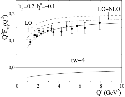
Figure 3: The scaled transition FF as a function of $Q^{2}$. The solid line corresponds to the sum of all the contributions (22). The data are taken from Refs. CELLO (the rectangles) and CLEO (the circles).

The scaled FF $Q^{2}F_{\pi\gamma}(Q^{2})$ and its different components are plotted in Fig. 3. As is seen, the leading order prediction for the FF in the QCD LCSR method considerably overshoots the data points. By including into consideration the NLO correction, one may only soften this discrepancy, but not remove it. In fact, the LCSR prediction with LO+NLO accuracy, for the values of the input parameters $b_{2}^{0},\;b_{4}^{0}$ shown in the figure, again overestimates the experimental data. It is evident that DAs with $b_{4}^{0}\geq 0$ will lead to a more great deviation from the experimental data than DAs with $b_{4}^{0}<0$. Therefore, the traditional treatment of the transition FF SY00 ; BMS03 would call for DAs with $b_{4}^{0}<0$, because the asymptotic twist-4 contribution is not strong enough to compensate the growth of the LO+NLO term if $b_{4}^{0}\geq 0$. In the renormalon approach the situation, in general, remains the same. This fact is connected with the dependence of the twist-4 term on the input parameters $b_{2}^{0},\;b_{4}^{0}$.

To understand this important point, it is instructive to explore the twist-4 contributions corresponding to different DAs. The relevant results are shown in Fig. 4. Here the dashed and solid curves are computed using the standard asymptotic function (27) and the renormalon-generated one (25) with $b_{2}^{0}=b_{4}^{0}=0,$ respectively. The difference between them is evident: almost in the whole region of the explored momentum transfers $Q^{2}\geq 1.8\;\mathrm{{GeV}^{2}}$ the higher conformal spin (renormalon) effects enhance the absolute value of the twist-4 contribution. The twist-4 terms corresponding to $b_{2}^{0}\neq 0,\;b_{4}^{0}\neq 0$ (the dot-dashed and dot-dot-dashed curves) in the region $1\ \mathrm{{GeV}^{2}\leq Q^{2}\leq 1.8\ {GeV}^{2}}$ are larger than the asymptotic contribution, whereas for $Q^{2}>1.8\ \mathrm{{GeV}^{2}}$ they run below both the solid and dashed curves. It is worth noting that at fixed $b_{2}^{0}=0.2$, curves $b_{4}^{0}=\pm 0.1$ (these values have been chosen as sample ones ) are close to each other: the sizeable difference between them appears only at $Q^{2}\geq 8\ \mathrm{{GeV}^{2}}$. This means that in the low-$Q^{2}$ region, DAs with $b_{4}^{0}=\pm 0.1$ reduce the LO+NLO contribution almost in the same manner, and this effect is smaller than the corresponding effect in the case of the asymptotic contribution. In the domain of the high $Q^{2}$, the twist-4 terms cut the LO+NLO result more effectively than the asymptotic twist-4 term, but because the LO+NLO ($b_{4}^{0}<0$) contribution itself is smaller than the LO+NLO ($b_{4}^{0}\geq 0$) one, it terns out that only DAs with $b_{4}^{0}<0$ lead to agreement with the data.

Figure 4: The twist-4 term as a function of $Q^{2}$. The dashed curve is computed using the function $\Phi_{asy}^{(4)}(u,Q^{2})$. The predictions for the twist-4 term obtained employing the renormalon-inspired DAs are shown by the solid and two broken lines. The correspondence between the lines and the input parameters is: the solid line, $b_{2}(\mu_{0}^{2})=0,\,\,b_{4}(\mu_{0}^{2})=0$; the dot-dashed line, $b_{2}(\mu_{0}^{2})=0.2,\,\,b_{4}(\mu_{0}^{2})=-0.1$; the dot-dot-dashed line, $b_{2}(\mu_{0}^{2})=0.2,\,\,b_{4}(\mu_{0}^{2})=0.1$.

In general, calculations of Ref. SY00 ; BMS03 correspond essentially to the ”minimal” model of the twist-4 effects, where the restriction to the lowest conformal spin probably underestimates the effect, while the renormalon model is a ”maximal” model, where these effects are probably somewhat overestimated. Therefore, the renormalon model for the twist-4 DAs allows us to put a theoretically justified bound on the twist-4 contribution to the pion transition form factor. The change in absolute value of the twist-4 term is not dramatic, as it may be expected. To quantify this statement we introduce the ratio $R(Q^{2})$,

$$R(Q^{2})=\frac{[F_{\pi\gamma}^{(4)}(Q^{2})]^{\mathrm{ren}}}{[F_{\pi\gamma}^{(4)}(Q^{2})]^{\mathrm{stand}}},$$

and demonstrate its numerical results in Fig. 5 for some selected values of $b_{2}^{0},\;b_{4}^{0}$.

Figure 5: The ratio $R(Q^{2})$ as a function of $Q^{2}$. The solid line corresponds to the input parameters $b_{2}(\mu_{0}^{2})=b_{4}(\mu_{0}^{2})=0$. The dashed line describes the same ratio, but for $b_{2}(\mu_{0}^{2})=0.2,\;b_{4}(\mu_{0}^{2})=0.1$, while the dot-dashed one corresponds to $b_{2}(\mu_{0}^{2})=0.2,\;b_{4}(\mu_{0}^{2})=-0.1$.

Figure 6: The $1\sigma$ area in the $b_{2}^{0}-b_{4}^{0}$ plane extracted from comparison of the CELLO and CLEO data with the LCSR prediction. The central solid rectangle denotes the point $b_{2}^{0}=0.27,\;b_{4}^{0}=-0.3$.

In Fig. 6 we plot the $1\sigma$ area in the $b_{2}^{0}-b_{4}^{0}$ plane, extracted at the scale $\mu_{0}^{2}=1\ \mathrm{{GeV}^{2}}$ in the result of the fitting procedure. One can see that this area stretches in the lower-half plane occupying a large region. The parameter $b_{2}^{0}$ varies within the limits

$$b_{2}^{0}\in[0.09,\,\,0.37],$$

whereas at some fixed $b_{2}^{0}$ the variation of $b_{4}^{0}$ is even larger. For example, at $b_{2}^{0}=0.2$, $b_{4}^{0}$ takes values in the region

$$b_{2}^{0}\in[-0.05,-\,\,0.45].$$

The $1\sigma$ region for the transition FF is shown in Fig. 7. In the fitting procedure we employ the CLEO data, and the two CELLO data points at $Q^{2}=1.26$ and $1.7\ \mathrm{{GeV}^{2}}$. The CELLO data have an important impact on the fitting procedure.

The central values for the parameters $b_{2}^{0}$ and $b_{4}^{0}$ extracted in this work are

$$b_{2}^{0}(1\ \mathrm{GeV}^{2})=0.27,\,\,b_{4}^{0}(1\ \mathrm{{GeV}^{2})=-0.3.}$$ (28)

It is difficult to present the $1\sigma$ region of the parameters by a simple formula, therefore we refrain from such attemps.

As is seen the curve in Fig. 7 in the low-$Q^{2}$ region decreases rapidly, deviating considerably from the CELLO point at $Q^{2}=0.94\;\mathrm{{GeV}^{2}}$: the DA (28)  describes the CELLO and CLEO data located only in the domain $1.26\;\mathrm{GeV}^{2}\leq Q^{2}\leq 7.9\;\mathrm{GeV}^{2}$.

Evolved to the normalization scale $\mu_{0}^{2}=5.76\ \mathrm{{GeV}^{2}}$, the parameters (28) become equal to

$$b_{2}^{0}\simeq 0.184,\,\,b_{4}^{0}\simeq-0.179.$$ (29)

Equation (29) can be compared with the predictions ($\mu_{0}^{2}=5.76\ \mathrm{GeV}^{2}$) from Ref. SY00 ,

$$b_{2}^{0}=0.19,\,\,b_{4}^{0}=-0.14,$$ (30)

and Ref. BMS03

$$b_{2}^{0}=0.2,\,\,b_{4}^{0}=-0.17.$$ (31)

From this analysis it becomes evident that both the standard and renormalon approaches predict the pion leading twist DA with a negative coefficient $b_{4}^{0}<0.$

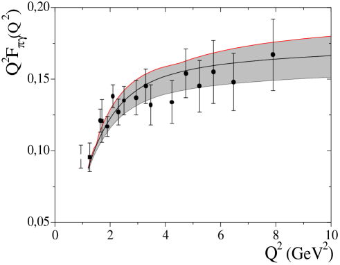
Figure 7: The form factor $Q^{2}F_{\pi\gamma}(Q^{2})$ as a function of $Q^{2}$. The shaded area demonstrates $1\sigma$ region for the transition FF. In the fitting procedure the solid data points have been used. The central solid curve corresponds to the parameters $b_{2}^{0}=0.27,\;b_{4}^{0}=-0.3$.

In our previous paper A02 we obtained the constraints on the pion leading twist DA from LCSR analysis of the pion electromagnetic FF. In calculations we employed the renormalon model for the twist-4 distributions (17), but took into account the evolution of the pion DAs with the lower than in the present work accuracy (i.e., with the LO accuracy). At the scale $\mu_{0}^{2}=1\ \mathrm{{GeV}^{2}}$ we found

$$b_{2}^{0}=0.2\pm 0.03,\,\,b_{4}^{0}=-0.03\pm 0.06.$$ (32)

The $1\sigma$ area depicted in Fig. 6 overlaps with  (32) (it is not shown in the figure) in the region determined by the following values of the parameters

$$b_{2}^{0}\simeq 0.2-0.23,\;b_{4}^{0}\simeq-0.05-(-0.09).$$

In general, an $1\sigma$ area for two quantities is not necessarily equal to the overlap region of two independent $1\sigma$ areas. Nevertheless, it is important, at least as the first approximation, to determine the pion DA that satisfactorily describes the both of these form factors. In order to get more precise estimate, $F_{\pi}(Q^{2})$ has to be calculated with higher accuracy, and a joint treatment of $F_{\pi\gamma}(Q^{2})$ and $F_{\pi}(Q^{2})$ must be performed. These tasks are beyond the scope of the present work.

V Conclusions

In this work we have used the pion renormalon-inspired higher twist DAs to calculate the twist-4 contribution to the transition form factor $F_{\pi\gamma}(Q^{2})$. The renormalon method has allowed us to express two– and three-particle twist-4 DAs in terms of the pion leading twist DA and one additional parameter $\delta^{2}$. In other words, in this method the twist-4 distributions are determined by the twist-2 one unambiguously, that restricts a freedom in the choice of DAs, increasing, at the same time, the predictive power and reliability of QCD results.

The higher twist distributions introduced in Ref. BGG04 embrace higher conformal spin effects which so far escaped attention. They are larger at the end points and, as expected, give rise to larger higher twist effects in exclusive reactions. Our results on the twist-4 contribution to the transition FF $F_{\pi\gamma}(Q^{2})$ confirm this assumption. Indeed, in the region of high momentum transfers the absolute value of the renormalon-generated twist-4 term exceeds the asymptotic one by a factor $1.5-2$. Nevertheless, the LCSR results obtained using the renormalon-inspired and standard DAs predict the pion leading twist DAs with $b_{4}^{0}<0$. Stated differently, effects due to higher conformal spin components of the twist-4 DAs remain under control and do not spoil the QCD LCSR method.

The new contribution of this work is that the renormalon approach has allowed one to put an upper bound on the twist-4 contribution to the light-cone sum rules and obtain estimates of the effects due to higher conformal spins.On the example of the $\gamma\gamma^{*}\to\pi^{0}$ transition, it also demonstrated limits of theoretical uncertainties inherent to our knowledge of exclusive processes.

*

Appendix A

The components $\varphi_{n}^{1}(u)$ and $\varphi_{n}^{2}(u)$ of the pion two-particle twist-4 DAs $\varphi_{1}^{(4)}(u,\mu_{F}^{2})$, $\varphi_{2}^{(4)}(u,\mu_{F}^{2})$ are given by the following expressions A02 :

$$\varphi_{0}^{1}(u)=\delta^{2}\left\{\overline{u}\left[\ln\overline{u}-\rm{Li}_{2}(\overline{u})\right]+u\left[\ln u-\rm{Li}_{2}(u)\right]-u\overline{u}+\frac{\pi^{2}}{6}\right\},$$

$$\varphi_{1}^{1}(u)=\delta^{2}\left\{\overline{u}\left[\left(1+\frac{\overline{u}}{2}-\frac{\overline{u}^{2}}{3}\right)\ln\overline{u}-\rm{Li}_{2}(\overline{u})\right]+u\left[\left(1+\frac{u}{2}-\frac{u^{2}}{3}\right)\ln u-\rm{Li}_{2}(u)\right]-\frac{5}{6}u\overline{u}+\frac{1}{2}u^{2}\overline{u}^{2}+\frac{\pi^{2}}{6}\right\},$$

$$\varphi_{2}^{1}(u)=\delta^{2}\left\{\overline{u}\left[\left(1+\overline{u}-\frac{2}{3}\overline{u}^{2}\right)\ln\overline{u}-\rm{Li}_{2}(\overline{u})\right]+u\left[\left(1+u-\frac{2}{3}u^{2}\right)\ln u-\rm{Li}_{2}(u)\right]-\frac{2}{3}u\overline{u}+\frac{5}{4}u^{2}\overline{u}^{2}+\frac{\pi^{2}}{6}\right\},$$

$$\varphi_{3}^{1}(u)=\delta^{2}\left\{\overline{u}\left[\left(1+\frac{3}{2}\overline{u}-\frac{7}{6}\overline{u}^{2}+\frac{1}{4}\overline{u}^{3}-\frac{1}{10}\overline{u}^{4}\right)\ln\overline{u}-\rm{Li}_{2}(\overline{u})\right]\right.$$

$$\left.+u\left[\left(1+\frac{3}{2}u-\frac{7}{6}u^{2}+\frac{1}{4}u^{3}-\frac{1}{10}u^{4}\right)\ln u-\rm{Li}_{2}(u)\right]-\frac{31}{60}u\overline{u}+\frac{257}{120}u^{2}\overline{u}^{2}-\frac{1}{3}u^{3}\overline{u}^{3}+\frac{\pi^{2}}{6}\right\},$$

$$\varphi_{4}^{1}(u)=\delta^{2}\left\{\overline{u}\left[\left(1+2\overline{u}-\frac{11}{6}\overline{u}^{2}+\frac{3}{4}\overline{u}^{3}-\frac{3}{10}\overline{u}^{4}\right)\ln\overline{u}-\rm{Li}_{2}(\overline{u})\right]\right.$$

$$\left.+u\left[\left(1+2u-\frac{11}{6}u^{2}+\frac{3}{4}u^{3}-\frac{3}{10}u^{4}\right)\ln u-\rm{Li}_{2}(u)\right]-\frac{23}{60}u\overline{u}+\frac{47}{15}u^{2}\overline{u}^{2}-\frac{41}{36}u^{3}\overline{u}^{3}+\frac{\pi^{2}}{6}\right\},$$

and

$$\varphi_{0}^{2}(u)=\delta^{2}\left[u^{2}\ln u+\overline{u}^{2}\ln\overline{u}+u\overline{u}\right],\;\;\varphi_{1}^{2}(u)=\delta^{2}\left[u^{2}\ln u+\overline{u}^{2}\ln\overline{u}+u\overline{u}+\frac{1}{2}u^{2}\overline{u}^{2}\right],$$

$$\varphi_{2}^{2}(u)=\delta^{2}\left[u^{2}\ln u+\overline{u}^{2}\ln\overline{u}+u\overline{u}+\frac{5}{6}u^{2}\overline{u}^{2}\right],\;\varphi_{3}^{2}(u)=\delta^{2}\left[u^{2}\ln u+\overline{u}^{2}\ln\overline{u}+u\overline{u}+\frac{13}{12}u^{2}\overline{u}^{2}-\frac{1}{6}u^{3}\overline{u}^{3}\right],$$

$$\varphi_{4}^{2}(u)=\delta^{2}\left[u^{2}\ln u+\overline{u}^{2}\ln\overline{u}+u\overline{u}+\frac{77}{60}u^{2}\overline{u}^{2}-\frac{13}{30}u^{3}\overline{u}^{3}\right],$$

where ${\rm{Li}}_{a}(x)=\sum_{n=1}^{\infty}x^{n}/n^{a}$.

The twist-4 contribution to the FF (24) can be formulated in terms of the twist-4 specrtal density $\rho^{(4)}(Q^{2},s)$:

$$F_{\pi\gamma}^{(4)}(Q^{2})=\frac{\sqrt{2}f_{\pi}}{3}\left[\frac{1}{m_{\rho}^{2}}\int_{0}^{s_{0}}ds\rho^{(4)}(Q^{2},s)\exp\left(\frac{m_{\rho}^{2}-s}{M^{2}}\right)+\frac{1}{Q^{2}}H^{(4)}(Q^{2})\right],$$

where

$$H^{(4)}(Q^{2})=\int_{s_{0}}^{\infty}\frac{ds}{s}Q^{2}\rho^{(4)}(Q^{2},s).$$

The twist-4 spectral density and the function $H^{(4)}(Q^{2})$ have the decompositions

$$\rho^{(4)}(Q^{2},s)=2\delta^{2}(Q^{2})\sum_{n=0}^{4}K_{n}(Q^{2})\rho_{n}^{4}(Q^{2},s)$$

and

$$H^{(4)}(Q^{2})=\frac{2\delta^{2}(Q^{2})}{Q^{2}}\sum_{n=0}^{4}K_{n}(Q^{2})H_{n}^{4}(Q^{2}).$$

The explicit expressions for the components of $\rho^{(4)}(Q^{2},s)$ and $H^{(4)}(Q^{2})$ are written down below (hereafter $t\equiv Q^{2}$):

$$\rho_{0}^{4}(t,s)=\frac{2}{(s+t)^{3}}\left\{s-t+2s\ln\left[\frac{s}{s+t}\right]-2t\ln\left[\frac{t}{s+t}\right]\right\},$$

$$\rho_{1}^{4}(t,s)=\frac{2}{(s+t)^{4}}\left\{s^{2}-t^{2}+2s^{2}\ln\left[\frac{s}{s+t}\right]-2t^{2}\ln\left[\frac{t}{s+t}\right]\right\},$$

$$\rho_{2}^{4}(t,s)=\frac{1}{3(s+t)^{5}}\left[6s^{3}+5s^{2}t-5st^{2}-6t^{3}\right]+\frac{2t(s-2t)}{(s+t)^{4}}\ln\left[\frac{t}{s+t}\right]+\frac{2s(2s-t)}{(s+t)^{4}}\ln\left[\frac{s}{s+t}\right],$$

$$\rho_{3}^{4}(t,s)=\frac{1}{3(s+t)^{7}}\left[6s^{5}+19s^{4}t+10s^{3}t^{2}-10s^{2}t^{3}-19st^{4}-6t^{5}\right]$$

$$+\frac{4t(s^{3}-st^{2}-t^{3})}{(s+t)^{6}}\ln\left[\frac{t}{s+t}\right]+\frac{4s(s^{3}+s^{2}t-t^{3})}{(s+t)^{6}}\ln\left[\frac{s}{s+t}\right],$$

$$\rho_{4}^{4}(t,s)=\frac{st(s-t)}{30(s+t)^{7}}\left[21s^{2}-65st+21t^{2}\right]$$

$$+\frac{1}{3(s+t)^{6}}\left\{t\left[5s^{3}-5s^{2}t-10st^{2}-6t^{3}\right]+s\left[6s^{3}+10s^{2}t+5st^{2}-5t^{3}\right]\right\}$$

$$+\frac{2t(3s^{3}-s^{2}t-st^{2}-2t^{3})}{(s+t)^{6}}\ln\left[\frac{t}{s+t}\right]+\frac{2s(2s^{3}+s^{2}t+st^{2}-3t^{3})}{(s+t)^{6}}\ln\left[\frac{s}{s+t}\right].$$

Here we introduce new notations

$$A=\ln\left[\frac{t}{s_{0}+t}\right],\;B=\ln\left[\frac{s_{0}}{s_{0}+t}\right],\;\;S(t)=\frac{2t(2A-1)}{s_{0}+t}+2B+4\left[\frac{\pi^{2}}{6}-{\rm{Li}}_{2}\left(\frac{s_{0}}{s_{0}+t}\right)\right],$$

and get:

$$H_{0}^{4}(t)=\frac{2}{(s_{0}+t)^{2}}\left[t^{2}(A-1)-ts_{0}-s_{0}(2t+s_{0})B\right]+S(t),$$

$$H_{1}^{4}(t)=\frac{1}{9(s_{0}+t)^{3}}\left[12t^{3}A-9t^{3}-ts_{0}(15t+6s_{0})-6s_{0}^{2}(3t+s_{0})B\right]+\frac{t^{2}(1+2A)}{(s_{0}+t)^{2}}+S(t),$$

$$H_{2}^{4}(t)=\frac{t^{4}}{6(s_{0}+t)^{4}}-\frac{t^{3}}{9(s_{0}+t)^{3}}+\frac{2}{(s_{0}+t)^{3}}\left[ts_{0}(s_{0}+t)+t^{3}A+s_{0}^{3}B\right]$$

$$+\frac{1}{(s_{0}+t)^{2}}\left[t(t-2s_{0})+2t^{2}A+2s_{0}(t-s_{0})B\right]+S(t),$$

$$H_{3}^{4}(t)=-\frac{t^{6}}{3(s_{0}+t)^{6}}+\frac{1}{5(s_{0}+t)^{5}}\left\{t\left[3t^{4}+4s_{0}(t^{3}+2t^{2}s_{0}+2ts_{0}^{2}+s_{0}^{3})\right]+4t^{5}A+4s_{0}^{5}B\right\}$$

$$-\frac{t^{4}(1+6A)}{6(s_{0}+t)^{4}}-\frac{3}{4(s_{0}+t)^{4}}\left[t^{4}+4t^{3}s_{0}+6t^{2}s_{0}^{2}+4ts_{0}^{3}+4s_{0}^{4}B\right]+\frac{t^{3}(-7+24A)}{9(s_{0}+t)^{3}}$$

$$+\frac{20}{9(s_{0}+t)^{3}}\left[t^{3}+3t^{2}s_{0}+3ts_{0}^{2}+3s_{0}^{3}B\right]+\frac{t^{2}(1+2A)}{(s_{0}+t)^{2}}-\frac{4s_{0}}{(s_{0}+t)^{2}}\left[t+(s_{0}-t)B\right]+S(t),$$

$$H_{4}^{4}(t)=-\frac{107t^{6}}{90(s_{0}+t)^{6}}+\frac{t^{5}(87+100A)}{50(s_{0}+t)^{5}}+\frac{2}{5(s_{0}+t)^{5}}\left[t^{5}+5t^{4}s_{0}+10t^{3}s_{0}^{2}+10t^{2}s_{0}^{3}+5ts_{0}^{4}+5s_{0}^{5}B\right]$$

$$-\frac{t^{4}(67+150A)}{60(s_{0}+t)^{4}}-\frac{15}{8(s_{0}+t)^{4}}\left[t^{4}+4t^{3}s_{0}+6t^{2}s_{0}^{2}+4ts_{0}^{3}+4s_{0}^{4}B\right]+\frac{t^{3}(-49+300A)}{90(s_{0}+t)^{3}}$$

$$+\frac{40}{9(s_{0}+t)^{3}}\left[t^{3}+3t^{2}s_{0}+3ts_{0}^{2}+3s_{0}^{3}B\right]+\frac{1}{2(s_{0}+t)^{2}}\left[t(t-14s_{0})+4t^{2}A+2s_{0}(6t-7s_{0})B\right]+S(t).$$

References

(1) G. P. Lepage and S. J. Brodsky, Phys. Lett. B 87, 359 (1979); Phys. Rev. D 22, 2157 (1980).
(2) A. V. Efremov and A. V. Radyushkin, Teor. Mat. Fiz.
42, 147 (1980) [Theor. Math. Phys. 42, 97 (1980)]; Phys.
Lett. B 94, 245 (1980).
(3) A. Duncan and A. H. Mueller, Phys. Rev. D 21,
1636 (1980).
(4) F. del Aguila and M. K. Chase, Nucl. Phys. B193,
517 (1981);
E. Braaten, Phys. Rev. D 28, 524 (1983);
E. P. Kadantseva, S. V. Mikhailov, and A. V. Radyushkin, Yad. Fiz.
44, 507 (1986) [Sov. J. Nucl. Phys. 44, 326 (1986)];
I. V. Musatov and A. V. Radyushkin, Phys. Rev. D 56, 2713
(1997);
B. Melic, D. Müller, and K. Passek-Kumericki, Phys. Rev. D 68, 014013 (2003).
(5) A. Khodjamirian, Eur. Phys. J. C 6, 477 (1999).
(6) A. Schmedding and O. Yakovlev, Phys. Rev. D 62,
116002 (2000).
(7) A. P. Bakulev, S. V. Mikhailov, and N. G. Stefanis,
Phys. Rev. D 67, 074012 (2003).
(8) S. S. Agaev, Phys. Rev. D 69, 094010 (2004).
(9) V. L. Chernyak and A. R. Zhitnitsky, Phys. Rep. 112, 173 (1984).
(10) V. Yu. Petrov, M. V. Polyakov, R. Ruskov, C. Weiss, and
K. Goeke, Phys. Rev. D 59, 114018 (1999);
M. Praszalowicz and A. Rostworowski, Phys. Rev. D 64, 074003
(2001);
A. E. Dorokhov, Pis’ma Zh. Eksp. Teor. Fiz. 77, 68 (2003) [JETP
Lett. 77, 63 (2003)].
(11) T. A. DeGrand and R. D. Loft, Phys. Rev. D 38, 954 (1988);
D. Daniel, R. Gupta, and D. G. Richards, Phys. Rev. D 43, 3715
(1991);
L. Del Debbio, M. Di Pierro, and A. Dougall, Nucl. Phys. Proc. Suppl.
119, 416 (2003);
M. Göckeler et al., QCDSF/UKQCD Coll., arxiv: hep-lat/0510089.
(12) V. M. Braun, G. P. Korchemsky, and D. Müller, Prog.
Part. Nucl. Phys. 51, 311 (2003).
(13) V. M. Braun and I. E. Filyanov, Z. Phys. C 48,
239 (1990).
(14) P. Ball, V. M. Braun, Y. Koike, and K. Tanaka, Nucl.
Phys. B529, 323 (1998);
P. Ball, V. M. Braun, Nucl. Phys. B543, 201 (1999);
P. Ball, J. High Energy Phys. 01, 010 (1999).
(15) J. R. Andersen, Phys. Lett. B 475, 141 (2000).
(16) V. M. Braun, E. Gardi, and S. Gottwald, Nucl. Phys.
B685, 171 (2004).
(17) S. S. Agaev, Phys. Rev. D 72, 074020 (2005).
(18) V. Braun and I. Halperin, Phys. Lett. B 328, 457
(1994);
V. M. Braun, A. Khodjamirian, and M. Maul, Phys. Rev. D 61, 073004
(2000);
J. Bijnens and A. Khodjamirian, Eur. Phys. J C 26, 67 (2002).
(19) H.-J. Behrend et al. (CELLO Collaboration), Z.
Phys. C 49, 401 (1991).
(20) J. Gronberg et al. (CLEO Collaboration), Phys. Rev.
D 57, 33 (1998).
(21) I. I. Balitsky and V. M. Braun, Nucl. Phys. B311,
541 (1989).
(22) V. L. Chernyak, A. R. Zhitnitsky, and I. R. Zhitnitsky, Yad.
Fiz. 38, 1074 (1983) [ Sov. J. Nucl. Phys. 38, 645 (1983)];
V. A. Novikov, M. A. Shifman, A. I. Vainstein, M. B. Voloshin, and V. I.
Zakharov, Nucl. Phys. B237, 525 (1984).
(23) F. M. Dittes and A. V. Radyushkin, Phys. Lett. B 134, 359 (1984);
M. H. Sarmadi, Phys. Lett. B 143, 471 (1984);
S. V. Mikhailov and A. V. Radyushkin, Nucl. Phys. B254, 89
(1985).
(24) I. I. Balitsky, V. M. Braun, and A. V. Kolesnichenko, Nucl.
Phys. B312, 509 (1989);
V. M. Braun and I. E. Filyanov, Z. Phys. C 44, 157 (1989);
V. L. Chernyak and I. R. Zhitnitsky, Nucl. Phys. B345, 137 (1990).
(25) A. P. Bakulev, S. V. Mikhailov, and N. G. Stefanis,
arxiv: hep-ph/0512119.
(26) M. A. Shifman, A. I. Vainstein, and V. I. Zakharov, Nucl.
Phys. B147, 385; B147 448 (1979).