${\cal{O}}(\alpha_{s}^{2})$ QCD corrections to inclusive jet production in deep inelastic scattering.

Abstract

We analyze the order $\alpha_{s}^{2}$ corrections to the single inclusive jet cross section in lepton-nucleon deep inelastic scattering. The full calculation is done analytically, in the small cone approximation, obtaining finite NLO partonic level cross sections for these processes. A detailed study of the different underlying partonic reactions is presented focusing in the size of the corrections they get at NLO accuracy, their relative weight, and the residual scale uncertainty they leave in the full cross section depending on the kinematical region explored. The dominant partonic process in very forward jet production is found to start at order $\alpha_{s}^{2}$, being effectively a lowest order estimate, with the consequent large factorization scale uncertainty, and the likelihood of non-negligible corrections at the subsequent order in perturbation theory.

Introduction

Over the last thirty years, the DGLAP DGLAP approach to parton dynamics has demonstrated itself as the most adequate tool for the description of the energy scale dependence of a variety of lepton-nucleon, and nucleon-nucleon processes over a wide kinematical range. Surprisingly, not just this approximation, but the lowest order in perturbation theory within this approach (LO) gives fairly accurate estimates for paradigmatic processes such as inclusive deep inelastic scattering (DIS), provided an energy or momentum scale of a few GeV characterizes them. The following order (NLO) often represents small corrections, required for precise comparisons, but not for the broad picture.

In the few last years high precision DIS experiments, with a wide kinematical coverage, and the ability to measure less inclusive processes, such as those performed by the ZEUS and H1 collaborations at HERA, have extended the tests on the dynamics of partons to the limits of their kinematical reach, looking for signatures of dynamics complementary to that described by the DGLAP approach. Illustrative examples of these tests are the measurements of final state hadrons Aktas:2004rb and jets jetsZ ; jetsH1 produced in DIS processes in the forward region, for which the LO DGLAP description fail to reproduce the data by an order of magnitude, and even NLO estimates fall short.

In a recent analysis Daleo:2004pn , it has been shown that the striking failure of the LO description in the case of forward hadrons by no means implies the breakdown of the DGLAP dynamics, but just the inadequacy of the LO picture, which simply does not include the dominant contribution to the measured cross section: the process in which an initial state gluon is knocked out from the nucleon, and also a gluon fragments into the detected final state hadron. Indeed, the NLO approximation, which takes into account these contributions, reproduce nicely the data Daleo:2004pn ; Kniehl:2004hf ; aure .

In the case of forward jets, the situation seems to be more compromised, because not only the LO estimates fail, but also NLO estimates fall short by a factor of two of the data jetsH1 . In reference jetsZ this feature together with the large scale dependence of NLO calculations, has been taken as indicative of the importance of higher order corrections. In order to improve the understanding of this situation, in the present paper we compute the order $\alpha_{s}^{2}$ corrections to the single inclusive jet cross section in lepton-nucleon deep inelastic scattering.

We perform the full calculation analytically, factoring out explicitly the remnant initial state singularities into the definition of parton densities, and dealing with those of final states in the small cone approximation, which assumes that the cone of the jet is narrow SCA . This approximation allows us to translate straightforwardly previous results on hadroproduction Daleo:2004pn to the case of jets, avoiding a rather cumbersome calculation and delicate numerical treatments for dealing with the collinear singularities. In Section I we outline the technical framework required for the small cone approximation (SCA) in the case of DIS.

The small cone technique approximates the full result obtained by NLO Monte Carlo generators, providing fairly good estimates for the cross sections with differences typically smaller than the theoretical uncertainties of the NLO estimate in the relevant kinematical range. We investigate in section II the range of validity of the small cone approximation against the full Monte Carlo NLO parton generators.

The finite cross sections obtained within the small cone approximation can be implemented in fast and stable codes, and simple to use. Exploiting the flexibility of them, in Section III we perform a detailed study of the different underlying partonic reactions and their main features: the size of the corrections they get at NLO accuracy, their relative weight, and the residual scale uncertainty they leave in the full cross section depending on the kinematical region explored.

Our main conclusion is that, as in the case of hadroproduction, the dominant partonic process in the most forward jet region accessed yet is the one with a gluon in the initial state and also a gluon as the main seed of the jet. This process starts at order $\alpha_{s}^{2}$, and makes the NLO effectively a lowest order estimate, with the consequent large factorization scale uncertainty, and the likelihood of non-negligible corrections at the subsequent order in perturbation.

I Single-jet-inclusive DIS cross section in the SCA.

In this section we outline the calculation of the single-jet-inclusive DIS cross section within the small cone approximation. This technique has been proposed SCA and used in computations of unpolarized single inclusive cross sections SCA2 , and more recently has been extended and validated for polarized proton-proton collisions Jager:2004jh .

The SCA can be thought as an expansion of the partonic cross section in terms of the half aperture $\delta$ of the cone over which the radiation around a given final state parton is integrated. This cone defines the jet at partonic level and the integration over it regularizes all final state collinear singularities. Keeping the most significant terms in this expansion, which is given by $a\,log(\delta)+b+{\cal{O}}(\delta^{2})$ and neglecting ${\cal{O}}(\delta^{2})$ and higher contributions, the expansion approximates surprisingly well the full results of the cone algorithm for cone radius up to $R\simeq 0.7$ in applications for proton-proton collisions Jager:2004jh .

The main advantage of the approach in the present case is that it is possible to relate analytical results on one-particle-inclusive cross sections calculated previously Daleo:2004pn , where all collinear divergences have already been canceled or factorized into parton densities and fragmentation functions, to the single-jet-inclusive cross section, for which the SCA gives an analytical expression as a function of the cone aperture. As in reference Daleo:2004pn , we restrict the discussion to the case of non-vanishing transverse momentum. The limit of vanishing transverse momentum requires a more involved treatment of collinear singularities Daleo:2003jf ; Daleo:2003xg . Schematically, we start with the finite one-particle-inclusive cross section, we undo the factorization of final state collinear singularities into fragmentation functions, which of course is not pertinent in the case of jet cross sections. Then, we add contributions that are not accounted for in the one-particle-inclusive fragmentation scheme, i.e. jets formed by two partons. The result is completely finite and for phenomenological applications can be convoluted with parton densities just as in the case of the one particle inclusive cross section. In practice, the approach is equivalent to having defined effective jet fragmentation functions that factorize the final state singularities.

I.1 Kinematics

In order to implement the approach in the case of DIS, we start defining the total cross section for the partonic process $a+l\rightarrow\mbox{1 Jet}+l^{\prime}+X$ with $n$ partons in the final state:

$$\frac{d\hat{\sigma}^{(n,i)}_{a\rightarrow{\mbox{\tiny 1 jet}}}}{dx_{B}\,dQ^{2}}=\frac{e^{2}}{\xi\,x_{B}^{2}\,S_{H}^{2}}\,\frac{1}{S_{n}}\,\int\left|{\cal M}^{(i)}_{a\rightarrow n}\right|^{2}\,\mbox{dPS}^{(n)}\,\left[\delta^{(3)}(\vec{p}_{\mbox{\tiny jet}}-\hat{p})\,2\,E_{\mbox{\tiny jet}}\right]\,\left[\frac{d^{3}p_{\mbox{\tiny jet}}}{2\,E_{\mbox{\tiny jet}}}\right]\,,$$ (1)

where $\hat{p}$ defines the jet momentum in terms of the momenta of the $n$ partons, $\xi$ is the momentum fraction of the parent hadron carried by parton $a$, $S_{H}=(P+l)^{2}$ is the squared energy of the collision in the lepton-proton center of mass, and $x_{B}$ the usual Bjorken variable. The index $i=M,L$ stands for metric and longitudinal contributions respectively. $S_{n}$ is a symmetry factor that account for identical partons in the final state.

Since the last two factors between square brackets in equation (1) are Lorentz invariant, we can evaluate the latter in the hadronic center of mass while the former in partonic center of mass. These frames are defined by $\vec{P}+\vec{q}=0$ and $\vec{p}_{a}+\vec{q}=0$, respectively, with $P$ and $p_{a}=\xi\,P$ the momenta of the initial state proton and parton respectively. In the hadronic center of mass frame, it is convenient to use the transverse energy, $E_{\perp}$, and pseudo-rapidity $\eta$, while in the partonic frame, we use the same variables as for the one-particle-inclusive case Daleo:2004pn :

$$y =-\frac{u}{Q^{2}+s} z =\frac{(Q^{2}+s)(s+t+u)}{s\,(Q^{2}+s+u)}=\frac{s+t+u}{s\,(1-y)}\,,$$ (2)

$$Y =-\frac{U}{Q^{2}+S} Z =\frac{(Q^{2}+S)(S+T+U)}{S\,(Q^{2}+S+U)}=\frac{S+T+U}{S\,(1-Y)}\,,$$ (3)

with

$$s =(q+p_{i})^{2} S =(q+P)^{2}\,,$$ (4)

$$t =-2\,q\cdot p_{\mbox{\tiny jet}} T =-2\,q\cdot p_{\mbox{\tiny jet}}=t\,,$$ (5)

$$u =-2\,p_{a}\cdot p_{\mbox{\tiny jet}} U =-2\,P\cdot p_{\mbox{\tiny jet}}=u/\xi\,.$$ (6)

Replacing the jet phase space in eq. (1) we find

$$\frac{d\hat{\sigma}^{(n)}_{a\rightarrow{\mbox{\tiny 1 jet}}}}{dx_{B}\,dQ^{2}}=\frac{1}{\xi}\,\int\frac{d\,\hat{\sigma}^{(n)}_{a\rightarrow{\mbox{\tiny 1 jet}}}}{dx_{B}\,dQ^{2}\,dy\,dz}\,\frac{\pi\,E_{\perp}}{\pi\,\frac{s}{2}\,(1-y)}\,dE_{\perp}\,d\eta\,,$$ (7)

where we have introduced

$$\frac{d\,\hat{\sigma}^{(n)}_{a\rightarrow{\mbox{\tiny 1 jet}}}}{dx_{B}\,dQ^{2}\,dy\,dz}=C_{n}\,\int\left|{\cal M}_{a\rightarrow n}\right|^{2}\,\mbox{dPS}^{(n)}\,\left[\delta^{(3)}(\vec{p}_{\mbox{\tiny jet}}-\hat{p})\,2\,E_{\mbox{\tiny jet}}\right]\,\left[\pi\,\frac{s}{2}\,(1-y)\right]\,.$$ (8)

and $C_{n}=e^{2}/(x_{B}^{2}\,S_{H}^{2}\,S_{n})$. We omit from now on the index $i$, since all the results that follow are valid for both metric and longitudinal components. Notice that equation (8) is valid in $d=4$ dimensions. Convolving the partonic cross section with appropriate parton densities $f_{a}(\xi)$, the hadronic cross section can be written as

$$\frac{1}{2\,E_{\perp}}\frac{d\sigma_{\mbox{\tiny 1 jet}}}{dx_{B}\,dQ^{2}\,dE_{\perp}\,d\eta}=\frac{1}{Q^{2}+S}\,\frac{1}{1-y}\,\int_{0}^{Z}\frac{dz}{1-z}\,\frac{f_{a}(\xi)}{\xi}\,\frac{d\hat{\sigma}^{(n)}_{a\rightarrow\mbox{\tiny 1 jet}}}{dx_{B}\,dQ^{2}\,dy\,dz}\,.$$ (9)

At variance with the one-particle-inclusive case, the variable $y$ is completely determined by $E_{\perp}$ and $\eta$,

$$y=Y=\frac{E_{\perp}}{S^{1/2}}\,e^{-\eta}\,,$$ (10)

while $z$ is not fixed. Equation (9) coincides with equation (13) in Daleo:2004pn when $D_{j}(\zeta)=\delta(1-\zeta)$.

I.2 Jet Contributions

In addition to the jet analog of the one-particle-inclusive contribution, where the detected final state jet is originated from the fragmentation of just one final state parton, while the other partons play as spectators and are integrated over, we have to consider additional contributions in the full jet cross section. The former will be denoted as $\hat{\sigma}_{a\rightarrow i}$, with initial state parton $a$ and fragmenting parton $i$. The latter include, on the one hand, contributions accounting for the situations in which the jet is formed by two partons which are denoted as $\hat{\sigma}_{a\rightarrow ij}$. On the other hand, we have to subtract configurations in which the cone that defines the jet contains two of the final state partons, that in the one particle inclusive case were nevertheless classified as $\hat{\sigma}_{a\rightarrow i}$. These contributions will be denoted as as $\hat{\sigma}_{a\rightarrow i(j)}$. Discriminated by their partonic content, we have the following ${\cal{O}}(\alpha_{s}^{2})$ contributions:

• $q\rightarrow g+g+q$:

  $$\begin{split}\left[d\hat{\sigma}^{(2g)}_{q\rightarrow q}-2\,d\hat{\sigma}_{q\rightarrow q(g)}\right]+\left[2\,d\hat{\sigma}_{q\rightarrow g}-2\,d\hat{\sigma}_{q\rightarrow g(g)}-2\,d\hat{\sigma}_{q\rightarrow g(q)}\right]+2\,d\hat{\sigma}_{q\rightarrow qg}+d\hat{\sigma}_{q\rightarrow gg}\,,\end{split}$$ (11)

• $q\rightarrow q+q^{\prime}+\bar{q}^{\prime}$:

  $$\left[d\hat{\sigma}^{(ij)}_{q\rightarrow q}\right]+\left[d\hat{\sigma}_{q\rightarrow q^{\prime}}-d\hat{\sigma}_{q\rightarrow q^{\prime}(\bar{q}^{\prime})}\right]+\left[d\hat{\sigma}_{q\rightarrow\bar{q}^{\prime}}-d\hat{\sigma}_{q\rightarrow\bar{q}^{\prime}(q^{\prime})}\right]+d\hat{\sigma}_{q\rightarrow q^{\prime}\bar{q}^{\prime}}\,,$$ (12)

• $q\rightarrow q+q+\bar{q}$:

  $$\left[2\,d\hat{\sigma}^{(ii)}_{q\rightarrow q}-2\,d\hat{\sigma}_{q\rightarrow q(\bar{q})}\right]+\left[d\hat{\sigma}_{q\rightarrow\bar{q}}-2\,d\hat{\sigma}_{q\rightarrow\bar{q}(q)}\right]+2\,d\hat{\sigma}_{q\rightarrow q\bar{q}}\,,$$ (13)

• $g\rightarrow g+q+\bar{q}$:

  $$\begin{split}&\left[d\hat{\sigma}_{g\rightarrow g}-d\hat{\sigma}_{g\rightarrow g(q)}-d\hat{\sigma}_{g\rightarrow g(\bar{q})}\right]+\left[d\hat{\sigma}_{g\rightarrow q}-d\hat{\sigma}_{g\rightarrow q(g)}\right]+\left[d\hat{\sigma}_{g\rightarrow\bar{q}}-d\hat{\sigma}_{g\rightarrow\bar{q}(g)}\right]+d\hat{\sigma}_{g\rightarrow gq}+d\hat{\sigma}_{g\rightarrow g\bar{q}}\,.\end{split}$$ (14)

where the $\hat{\sigma}_{a\rightarrow i}$ terms are those already taken into account in the one-particle-inclusive cross section, with the adequate combinatoric prefactors. Notice that cross sections with identical partons in the final state get a symmetry factor, so we have to add them to the corresponding matrix elements, before factorization. For instance, all the matrix elements involved in the first and third reaction have to be multiplied by $1/2$ due to the presence of two gluons or two identical quarks in the final state.

In the small cone approximation it is customary to neglect ${\cal{O}}(\delta^{2})$ contributions in the cross section, which means we can approximate the matrix elements associated to two partons forming a jet with the corresponding collinear limit. This simplifies drastically the calculation because in this limit the ${\cal{O}}(\alpha_{s}^{2})$ $1\longrightarrow 3$ matrix elements factorize into ${\cal{O}}(\alpha_{s})$ $1\longrightarrow 2$ matrix elements times LO splitting functions. In the list above, we have skipped terms that vanish in this approximation. For example, in the second reaction $q\rightarrow q+q^{\prime}+\bar{q}^{\prime}$, the matrix elements vanish in the limit in which quark $q$ is collinear with any of $q^{\prime}$ or $\bar{q}^{\prime}$.

Restricting ourselves to the limit when partons $j$ and $k$ become collinear, for both $d\hat{\sigma}_{a\rightarrow j(k)}$ and $d\hat{\sigma}_{a\rightarrow jk}$, the corresponding matrix elements are given by Catani:1998nv ($d=4+\epsilon$):

$$\left|{\cal M}_{a\rightarrow ijk}\right|^{2}\stackrel{{\scriptstyle j\parallel k}}{{\longrightarrow}}\frac{2}{s_{jk}}\,4\,\pi\,\mu^{-\epsilon}\,\alpha_{s}\,\left|{\cal M}_{a\rightarrow iJ}\right|^{2}\,\hat{P}_{J\rightarrow jk}(\alpha,\epsilon)\,,$$ (15)

where the momenta of the parent parton, $J$, is defined in terms of those of partons $j$ and $k$:

$$p_{j}^{\mu} =\alpha\,p_{J}^{\mu}+k_{\perp}^{\mu}-\frac{k_{\perp}^{2}}{\alpha}\,\frac{n^{\mu}}{2\,p_{J}\cdot n}\,, p_{k}^{\mu} =(1-\alpha)\,p_{J}^{\mu}-k_{\perp}^{\mu}-\frac{k_{\perp}^{2}}{1-\alpha}\,\frac{n^{\mu}}{2\,p_{J}\cdot n}\,,$$ (16)

with $p_{J}\cdot k_{\perp}=n\cdot k_{\perp}=0$ and $p_{J}^{2}=n^{2}=0$. Consequently

$$p_{J}=\frac{(1-\alpha)\,p_{k}-\alpha\,p_{j}}{1-2\,\alpha}-k_{\perp}.$$ (17)

Notice that due to the singularities (poles in $\epsilon$) arising from the $s_{jk}$ factor in the denominator when integrating over the phase space, we need the splitting functions in (15) up to order $\epsilon$. The poles in $\alpha=1$ in the diagonal kernels ($J=j$) will give rise poles in $z=0$.

I.3 $d\hat{\sigma}_{a\rightarrow j(k)}$ contributions

As we mentioned, these contributions correspond to configurations where the jet is formed solely by parton $j$, but parton $k$ lies within the cone. They can be computed along the lines of what has been done in reference Jager:2004jh but now for DIS kinematics. In the partonic center of mass frame we have

$$s_{jk} =2\,p_{j}\cdot p_{k}=2\,E_{j}\,E_{k}\,(1-\cos\theta_{jk})\,, E_{j} =\frac{s^{1/2}}{2}\,(1-z\,(1-y))\,, E_{k} \simeq\frac{s^{1/2}}{2}\,z\,(1-y)\,,$$ (18)

while the collinear limit implies $\alpha=1-z\,(1-y)$. Then, we can write the matrix element for $d\hat{\sigma}_{a\rightarrow j(k)}$ as

$$\begin{split}\left|{\cal M}_{a\rightarrow ijk}\right|^{2}\stackrel{{\scriptstyle j\parallel k}}{{\longrightarrow}}&\frac{1-z\,(1-y)}{z\,(1-y)}\,\frac{1}{E_{j}^{2}\,(1-\cos\theta_{jk})}\,\hat{P}_{J\rightarrow jk}(\alpha,\epsilon)\,4\,\pi\,\mu^{-\epsilon}\,\alpha_{s}\,\left|{\cal M}_{a\rightarrow iJ}\left(s,y^{\prime}=\frac{y}{1-z\,(1-y)}\right)\right|^{2}\,.\end{split}$$ (19)

For the phase space we have,

$$\begin{split}\mbox{dPS}^{(3)}&=\frac{\pi\,s}{(4\,\pi)^{4}}\,\frac{2^{4-d}}{\Gamma^{2}\left(\frac{d-2}{2}\right)}\,\left(\frac{s}{4\,\pi}\right)^{d-4}\,\sin^{d-4}\theta_{jk}\,d\cos\theta_{jk}(1-y)^{2}\,z\,\left((1-y)^{3}\,y\,z^{2}\,(1-z)\right)^{(d-4)/2}dy\,dz\,,\end{split}$$ (20)

and combining with the matrix elements in (19), we have

$$\frac{d\hat{\sigma}_{a\rightarrow j(k)}}{dx_{B}\,dQ^{2}\,dy\,dz}=\frac{1}{S_{n}}\,\left(\frac{\delta}{2}\right)^{\epsilon}\,{\cal F}_{a\rightarrow iJ}\,\left[(1-y)^{1+\epsilon}\,z^{\epsilon}\,\hat{P}_{J\rightarrow jk}(\alpha=1-z\,(1-y),\epsilon)\right]\,,$$ (21)

where

$$\begin{split}{\cal F}_{a\rightarrow iJ}&=\frac{e^{2}}{x_{B}^{2}\,S_{H}^{2}}\,\frac{\alpha_{s}}{(4\,\pi)^{2}}\,\frac{2}{\epsilon}\,\frac{1}{\Gamma^{2}\left(1+\frac{\epsilon}{2}\right)}\,\frac{\left(y\,(1-y)\,(1-z)\right)^{\epsilon/2}}{1-z\,(1-y)}\,\left(\frac{s}{4\,\pi\,\mu^{2}}\right)^{\epsilon}\times\mu^{\epsilon}\,\left|{\cal M}_{a\rightarrow iJ}\left(s,y^{\prime}=\frac{y}{1-z\,(1-y)}\right)\right|^{2}\,.\end{split}$$ (22)

Notice that with this notation, the variables $y$ and $z$ in ${\cal F}_{a\rightarrow iJ}(s,y,z)$ are defined in terms of the second parton in the final state $J$. As mentioned above, the poles in $\alpha=1$ in the diagonal kernels, appear as poles in $z=0$ (notice that $y=1$ is protected by the $1-y$ factor coming from the phase space). This poles have to be prescribed as usual, leading to double poles in $\epsilon$, together with the appearance of $\delta(z)$ and ‘plus’ distributions in $z=0$. The double poles cancel with terms coming from $d\sigma_{a\rightarrow jk}$, whereas the remaining $1/\epsilon$ poles cancel terms generated when the fragmentation function factorization of the one-particle-inclusive cross section is undone.

I.4 $d\hat{\sigma}_{a\rightarrow jk}$ contributions

These terms account for jets formed by two partons, $j$ and $k$. In the collinear limit (15) we have:

$$E_{\mbox{\tiny jet}}=E_{J}\simeq\frac{E_{j}}{\alpha}\simeq\frac{E_{k}}{1-\alpha}\,,$$ (23)

where $\alpha$ is again the momentum fraction in the splitting function. The phase space in this case is

$$\begin{split}\mbox{dPS}^{(3)}&=\frac{1}{(4\,\pi)^{3}}\,\frac{1}{\Gamma^{2}\left(\frac{d-2}{2}\right)}\,\left(\frac{s}{4\,\pi}\right)^{d-4}\,\delta(z)\,(y\,(1-y))^{(d-4)/2}\left(\frac{E_{\mbox{\tiny jet}}}{\sqrt{s}}\right)^{d-4}\,\frac{E_{\mbox{\tiny jet}}^{3}}{E_{k}}\,\alpha^{d-3}\,d\alpha\,\sin^{d-3}\theta_{j}\,d\theta_{j}\,dy\,dz\,,\end{split}$$ (24)

where we have chosen the frame in such a way that the jet momentum is oriented in the $z$ axis. This result exhibits some differences with the previous case. Due to the presence of the $\delta(z)$ function, the $d\hat{\sigma}_{a\rightarrow jk}$ pieces only contribute at $z=0$. On the other hand, now we have to perform explicitly the integration over the argument of the splitting functions, $\alpha$. In addition, we see that the only dependence on the angle in the matrix element comes, again, form the $s_{jk}$ denominator. However, now we are integrating over $\theta_{j}$ and not over $\theta_{jk}$. As in Jager:2004jh , we find

$$\theta_{j} \simeq(1-\alpha)\,\theta_{jk}\,, \theta_{k} =\alpha\,\theta_{jk}\,.$$ (25)

and the integration limit over $\theta_{j}$ is given by $\delta$ if $E_{j}<E_{k}$ and by $(1-\alpha)/\alpha\,\delta$ if $E_{j}>E_{k}$. Performing the angular integrals in the partonic center of mass frame,

$$\frac{d\hat{\sigma}_{a\rightarrow jk}}{dx_{B}\,dQ^{2}\,dy\,dz}=\frac{1}{S_{n}}\,\left(\frac{\delta}{2}\right)^{\epsilon}\,{\cal F}_{a\rightarrow iJ}\,\delta(z)\,\int_{0}^{1}d\alpha\,\left[\Theta\left(\frac{1}{2}-\alpha\right)\,\alpha^{\epsilon}+\Theta\left(\alpha-\frac{1}{2}\right)\,(1-\alpha)^{\epsilon}\right]\hat{P}_{J\rightarrow jk}(\alpha,\epsilon)\,,$$ (26)

I.5 Cancellation of singularities.

The last step consists in reverting the factorization of final state collinear singularities already done in the finite one-particle-inclusive cross section. The simplest way to implement this step is simply to add to the already finite one-particle-inclusive cross section the terms we customary factorize into fragmentation functions, with the opposite sign. This provides a check of the whole calculation, as the simple poles still appearing in the correction terms have to cancel when we add these contributions.

The terms that have to be added can be read from the following factorization prescription formula for the partonic cross sections at first order, when renormalizing fragmentation functions:

$$\begin{split}\frac{d\hat{\sigma}_{a\rightarrow i}}{dx_{B}\,dQ^{2}\,dy}\longrightarrow&\,\frac{\alpha_{s}}{2\,\pi}\left(-\frac{2}{\epsilon}\right)\,\frac{1-y}{1-z\,(1-y)}\,\frac{\Gamma(1+\epsilon/2)}{\Gamma(1+\epsilon)}\left(\frac{M_{D}^{2}}{4\,\pi\mu^{2}}\right)^{\epsilon/2}\frac{d\hat{\sigma}_{a\rightarrow i}}{dx_{B}\,dQ^{2}\,dy}\sum_{k}\,P_{i\rightarrow jk}(1-z\,(1-y))\,.\end{split}$$ (27)

The splitting kernels in (27) are the regularized ones in 4 dimensions. The Born level cross sections are, in turn, given by:

$$\begin{split}\frac{d\hat{\sigma}_{a\rightarrow i}}{dx_{B}\,dQ^{2}\,dy}&=\frac{e^{2}}{x_{B}^{2}\,S_{H}^{2}}\,\frac{1}{8\,\pi}\,\frac{1}{\Gamma(1+\epsilon/2)}\,\left(\frac{s}{4\,\pi\mu^{2}}\right)^{\epsilon/2}\,y^{\epsilon/2}\,(1-y)^{\epsilon/2}\,\mu^{\epsilon}\,\sum_{j}\left|{\cal M}_{a\rightarrow ij}\right|^{2}\,.\end{split}$$ (28)

The additional factor of $1/\xi$ in the hadronic cross section is simply re-expressed in terms of the new variables and factors out everywhere.

Taking into account all the first order cross sections, we have the following contributions coming from reverting final state factorization

$$\begin{split}d\hat{\sigma}_{ct}=&d\hat{\sigma}_{q\rightarrow(qg)}+d\hat{\sigma}_{q\rightarrow(gq)}+d\hat{\sigma}_{q\rightarrow(gg)}+\sum_{q^{\prime}}\left(d\hat{\sigma}_{q\rightarrow(q^{\prime}\bar{q^{\prime}})}+d\hat{\sigma}_{q\rightarrow(\bar{q^{\prime}}q^{\prime})}\right)\\ &+d\hat{\sigma}_{g\rightarrow(qg)}+d\hat{\sigma}_{g\rightarrow(\bar{q}g)}+d\hat{\sigma}_{g\rightarrow(gq)}+d\hat{\sigma}_{g\rightarrow(g\bar{q})}\,,\end{split}$$ (29)

where we have introduced the notation $d\sigma_{a\rightarrow(jk)}$:

$$\begin{split}\frac{d\hat{\sigma}_{a\rightarrow(jk)}}{dx_{B}\,dQ^{2}\,dy\,dz}==\frac{\Gamma^{2}(1+\epsilon/2)}{\Gamma(1+\epsilon)}\,\left(\frac{M_{D}^{2}}{s}\right)^{\epsilon/2}\,{\cal F}_{a\rightarrow iJ}\times(1-y)\,(1-z\,(1-y))^{-\epsilon}\,P_{J\rightarrow jk}(1-z\,(1-y))\,.\end{split}$$ (30)

Notice that we have already added a minus sign to these contributions, as they must be subtracted to recover the original, un-factorized, one-particle-inclusive cross section. We also took into account the fact that at first order, the sum in eq. (28) contains only one term.

As mentioned, doubles poles must cancel explicitly between the $\sigma_{a\rightarrow j(k)}$ and $\sigma_{a\rightarrow jk}$ contributions. The remaining single poles must cancel with $d\sigma_{a\rightarrow(jk)}$. To make this cancellations more transparent, it is convenient to group the different contributions in eqs. (11)-(14) and the ones in (29). Starting with the quark initiated reactions and omitting $d\sigma_{a\rightarrow j}$ contributions (which are already finite) we have

$$\begin{split}f_{q}\rightarrow&-\Big{[}2\,d\hat{\sigma}_{q\rightarrow g(q)}-d\hat{\sigma}_{q\rightarrow(gq)}\Big{]}-n_{f}\,\Big{[}d\hat{\sigma}_{q\rightarrow q^{\prime}(\bar{q}^{\prime})}+d\hat{\sigma}_{q\rightarrow\bar{q}^{\prime}(q^{\prime})}-d\hat{\sigma}_{q\rightarrow(q^{\prime}\bar{q}^{\prime})}-d\hat{\sigma}_{q\rightarrow(\bar{q}^{\prime}q^{\prime})}\Big{]}\\ &-\Big{[}2\,d\hat{\sigma}_{q\rightarrow q(g)}-2\,d\hat{\sigma}_{q\rightarrow qg}-d\hat{\sigma}_{q\rightarrow(qg)}\Big{]}-\Big{[}2\,d\hat{\sigma}_{q\rightarrow g(g)}-d\hat{\sigma}_{q\rightarrow gg}-d\hat{\sigma}_{q\rightarrow(gg)}-\,n_{f}\,d\hat{\sigma}_{q\rightarrow q^{\prime}\bar{q}^{\prime}}\Big{]}\,.\end{split}$$ (31)

For the gluon initiated reactions, we have:

$$\begin{split}f_{g}\rightarrow&-\Big{[}d\hat{\sigma}_{g\rightarrow g(q)}-d\hat{\sigma}_{g\rightarrow(gq)}\Big{]}-\Big{[}d\hat{\sigma}_{g\rightarrow g(\bar{q})}-d\hat{\sigma}_{g\rightarrow(g\bar{q})}\Big{]}-\Big{[}{d\hat{\sigma}_{g\rightarrow q(g)}}-{d\hat{\sigma}_{g\rightarrow qg}}-d\hat{\sigma}_{g\rightarrow(qg)}\Big{]}\\ &-\Big{[}{d\hat{\sigma}_{g\rightarrow\bar{q}(g)}}-{d\hat{\sigma}_{g\rightarrow\bar{q}g}}-d\hat{\sigma}_{g\rightarrow(\bar{q}g)}\Big{]}\,.\end{split}$$ (32)

In Appendix I, we list the results corresponding to the cancellations for each of the terms in square brackets, which completes the calculation.

II Comparison with Monte Carlo results.

Having obtained the finite expressions for the NLO corrections in the SCA, in this section we investigate the accuracy of the approximation. In Figure 1 we compare the outcome of the SCA for the single jet inclusive DIS cross section with a full Monte Carlo NLO calculation of disent . The jets are reconstructed in the Breit frame and the rates between both results are computed in the typical kinematic range of forward jet DIS experiments at HERA. Jets are defined using the inclusive $k_{T}$ cluster algorithm ES in the Monte Carlo, and a cone radius of $R=0.7$ for the SCA value for which the agreement between both jet definitions is maximized.

The rates are presented as a function of the transverse momentum $E_{T}$ and rapidity $\eta$ of the jet, both measured in the laboratory frame, and Bjorken momentum fraction $x_{B}$

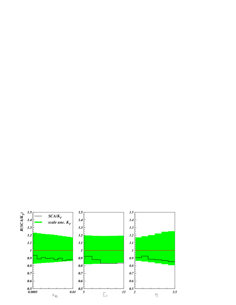
Figure 1: Ratio of NLO SCA estimate and the full Monte Carlo prediction with $k_{T}$ jet reconstruction.

In both cases we use the MRST02 NLO set of parton densities MRST02 and we compute $\alpha_{s}$ at NLO fixing $\Lambda_{QCD}$ as in the MRST analysis so $\alpha_{s}(M_{Z})=0.1197$. The rapidity variable varies between $2.0$ and $3.5$, the Bjorken variable spans the interval between $0.0005$ and $0.01$, the transverse momentum of the jet starts at $5\,\mbox{GeV}$, and $Q^{2}$ ranges from $20$ to $100\,\mbox{GeV}^{2}$.

As it has been observed in references SCA2 and Jager:2004jh , for hadronic collisions, even for rather large cone radius the SCA gives acceptable approximations within less than a ten percent of the full Monte Carlo result. This is also the case for DIS and the rates show a very mild dependence in the kinematical variables.

Certainly, the accuracy of SCA is the better for smaller cone radius, however the error introduced by the approximation with $R=0.7$, which is of the order of a 10 %, always underestimating the cross section and with a very mild dependence on the relevant variables, is comparable or smaller than the theoretical uncertainty coming from the particular choice of the factorization and renormalization scales, characteristic of the NLO corrections in this kinematical region. As we show in the following section, this means that we can safely use the SCA results as an estimate of the size and behavior of the NLO corrections. For comparison, in the Figure 1, we also plot as a band the uncertainty resulting from varying the factorization and renormalization scale by a factor of two in the full Monte Carlo result.

III Phenomenological consequences

Having established our level of confidence in the SCA results, we proceed analyzing the distinctive features of the NLO corrections in the forward region. We do the analysis in the typical kinematic region tested by DESY experiments, where large higher order effects have been observed.

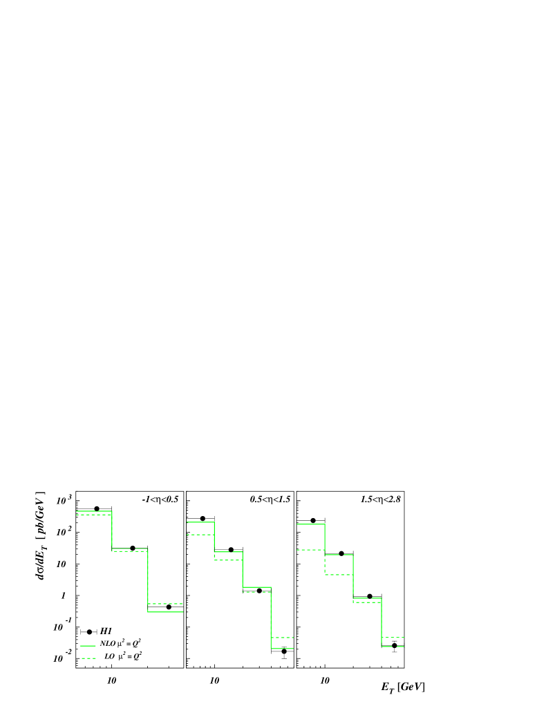
Figure 2: Size of NLO corrections as a function of $E_{T}$ for different rapidity regions.

The most striking of these features is the size of the NLO corrections as the rapidity of the jets increases. In Figure 2 we show both LO an NLO partonic level expectations coming from the SCA approach in three different regions of rapidity for $5<Q^{2}<100\mbox{GeV}^{2}$ and $0.2<y_{el}<0.6$ as a function of transverse jet momentum. Clearly, NLO corrections, which are moderate for central rapidities, become significantly large in the forward region. This feature is due to a suppression of the LO contributions rather than to an increase in rapidity of the cross sections. K-factors can exceed an order of magnitude there, invalidating the lowest order approximation. We have included for reference the data obtained by H1 in that kinematical range Adloff:2002ew , although one should keep in mind that for a precise comparison hadronization effects should also be taken into account.

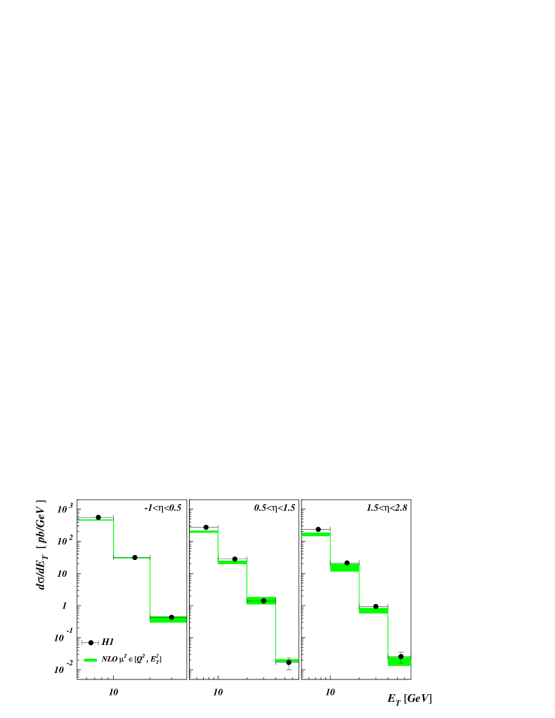
Figure 3: Scale uncertainty in NLO corrections as a function of $E_{T}$ for different rapidity regions.

Another interesting feature of NLO corrections to be taken into account is the rather large uncertainty these corrections show associated with the choice for the factorization and renormalization scales. In Figure 2 we adopted $\mu^{2}=Q^{2}$ for the factorization and renormalization scale. The choice for these scales is in principle arbitrary; the differences found in any perturbative estimate coming from some particular choice for the scale or other, become smaller as more terms in the perturbation series are included. In inclusive DIS $Q^{2}$ is the typical choice, while $E_{T}^{2}$ is the one favored in jet physics. In Figure 3 we plot the uncertainty bands corresponding to vary the scale from $Q^{2}$ to $E_{T}^{2}$, the two main scales of the process under consideration.

With such a large scale uncertainty, any particular choice will probably lead to miss the data at some point. One possible choice in these cases is to take the average between them, which leads to an intermediate estimate within the band. Again we can see that in the most forward bin, the uncertainty associated to the choice of the scale becomes more prominent and may be as large as a factor of two.

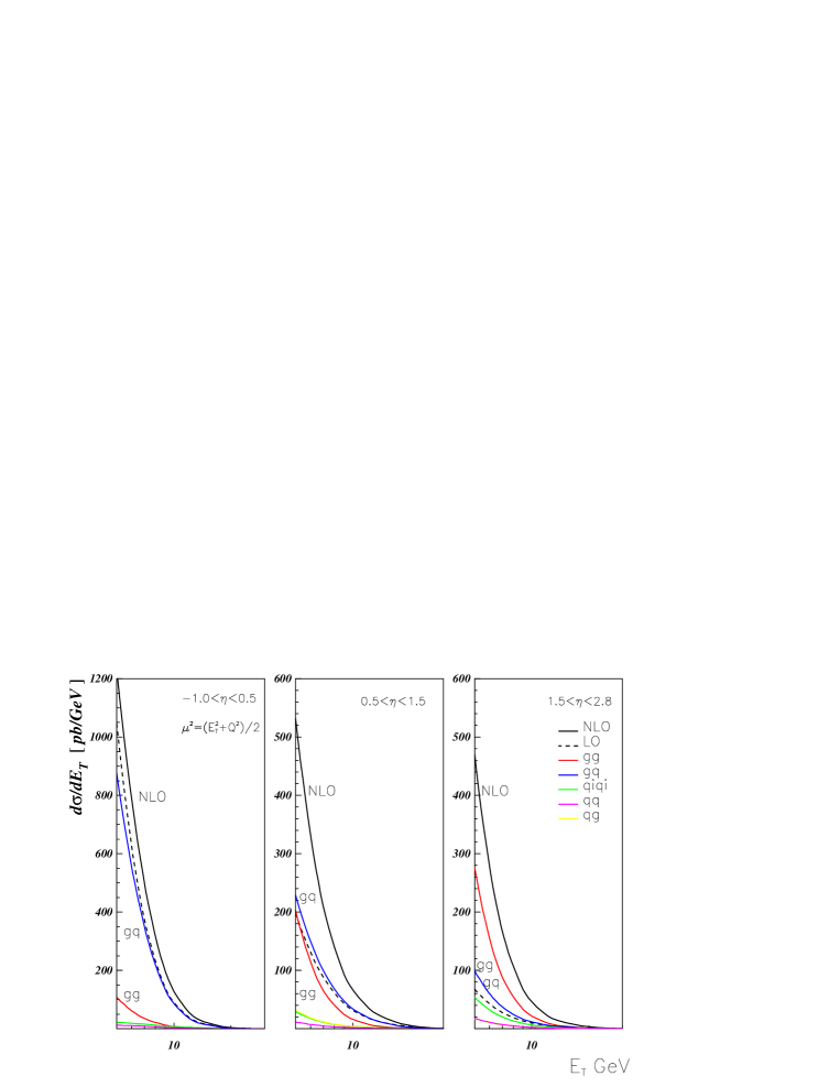
Figure 4: Partonic contributions as a function of $E_{T}$ for different rapidity regions.

In order to understand the correlation between higher order corrections and rapidity, it is useful to discriminate the different partonic contributions, classifying them as in the one particle inclusive case in terms of the initial state parton, $i$, and the one taken as the seed for the jet, $j$, as in $\sigma_{i\rightarrow j}$. The additional contributions coming from the first two terms in Eq.(32) were added to the $\sigma_{g\rightarrow g}$ contribution, the remaining terms in that equation were associated to $\sigma_{g\rightarrow q}$. Contributions in Eq. (31) were taken together with $\sigma_{q\rightarrow g}$.

In Figure 4 we show the different partonic contributions in the three rapidity regions. While in the central region the LO contribution is very close to the full NLO estimate, in the forward region it is significantly smaller. In the former region, the cross section is dominated by the $\sigma_{g\rightarrow q}$ contributions (an initial state gluon with a quark originating the jet), which are already present at LO, while in the latter the dominants are $\sigma_{g\rightarrow g}$, which are pure NLO, shown in Figure 5. These contributions start at order $\alpha_{s}^{2}$ so the NLO result is its lowest order estimate. The reason for their dominance over the LO is just the kinematical region chosen which suppress LO configurations. The dominance of the $\sigma_{g\rightarrow g}$ over $\sigma_{g\rightarrow q}$ NLO contributions can be traced back to the negative ’plus’ contributions which are proportional $C_{F}^{2}$ in the case of the former and to $C_{F}C_{A}$ for the latter.

Figure 5: Gluon initiated contributions at ${\cal{O}}(\alpha_{s}^{2})$

Since the dominant partonic process in the forward region is accounted, at order $\alpha_{s}^{2}$, only by only its lowest order contribution, it is effectively a LO estimate and most probably receives significant higher order corrections. The first order corrections for other partonic processes in this kinematic region rise typically to 50% effects, so it would not be surprising that the NLO estimate falls short of the data, specially if a more stringent kinematic range is explored.

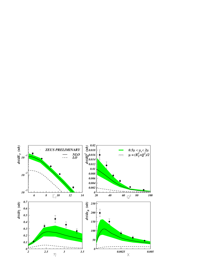
Figure 6: NLO estimates against ZEUS very forward preliminary data zeusdis

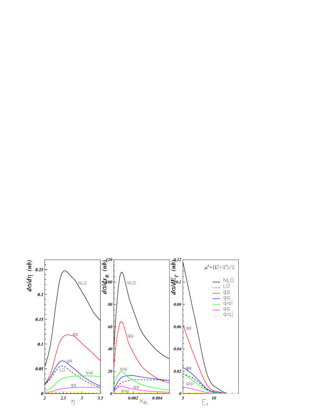
Figure 7: Partonic contributions in Zeus very forward measurement zeusdis

This is precisely what ZEUS has reported in preliminary analyses of measurements in the very forward region zeusdis .

In Figure 6 we plot the NLO estimates for the cross section as distributions in different variables together with ZEUS preliminary data zeusdis . The estimate correspond to rapidities between $2.0$ and $3.5$, the Bjorken variable in the interval $0.0004$ and $0.005$, the transverse momentum of the jet starting at $5\,\mbox{GeV}$, and the virtuality of the photon $Q^{2}$ range from $20$ to $100\,\mbox{GeV}^{2}$. The NLO estimate falls short of the preliminary data, and only allowing a rather large scale uncertainty it may be considered consistent with the measurements, specially at small $x_{B}$.

Further insight is obtained analyzing the different partonic contributions as a function of $\eta$ and $x_{B}$. In Figure 7 it can be noticed that the $\sigma_{g\rightarrow g}$ contributions dominate the cross section, specially at low $x_{B}$ where the gluon parton density grows dramatically and in the middle of the rapidity range. In these two regions one can expect the first order corrections to these processes, starting at NNLO, to be significant. In fact, it is there where the NLO estimate can be more distant to the data with a particular choice for the scale, as can be seen when comparing with the preliminary data in Ref. zeusdis . At larger $x_{B}$ and $\eta$, $\sigma_{g\rightarrow g}$ contributions decrease, even below the LO contribution, but the other NLO contributions keep the total NLO effect very large. Of these contributions, the most prominent is $\sigma^{(ij)}_{q\rightarrow q}$, that corresponds to diagrams, like the ones in Figure 8, where the two quarks lines have different flavours, but where the quark that initiates the jet has the same flavour as the one in the initial state.

Figure 8: Typical quark initiated contributions at ${\cal{O}}(\alpha_{s}^{2})$

Going to even higher rapidities, these last contributions eventually dominate the cross section, with the LO estimate being completely suppressed as shown in Figure 9. In this region, with the two dominant contributions being computed at the lowest order, the scale uncertainty of the NLO estimate is twice as large as that found in the rapidity region of Figure 7.

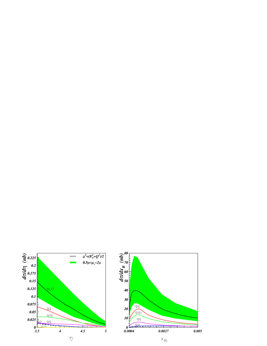
Figure 9: Partonic contributions in an extremely forward region

IV Conclusions

We have computed the single jet inclusive deep inelastic scattering cross section at ${\cal{O}}(\alpha_{s}^{2})$ in the small cone approximation. We found that this approach approximates the full NLO Monte Carlo results within a 10% accuracy, error which is fairly moderate compared to the main source of theoretical uncertainty, the scale dependence.

As in the case of hadroproduction in deep inelastic scattering, we have found that the dominant partonic processes in very forward jet production start at order $\alpha_{s}^{2}$, being effectively a lowest order estimate. As in any lowest order calculation, there is a large factorization scale uncertainty which can not be neglected, and it is likely that there will be large corrections at the subsequent order in perturbation. Although taking into account this large dependence on the choice for the scale, one can bring agreement between data and NLO estimates, the difference between them for a particular choice is maximal precisely where the partonic contributions computed for the first time are dominant. This feature is expected to be even more apparent at higher rapidities, and the corresponding measurements will constitute an obligatory benchmark for the study of QCD at NNLO.

V Acknowledgments.

We warmly acknowledge D. de Florian, C. A. García Canal, C. Glasman and Juan Terrón for comments and suggestions. We also thank C.Glasman for providing us ZEUS data. The work of A.D. was supported in part by the Swiss National Science Foundation (SNF) through grant No. 200020-109162 and by the Forschungskredit der Universität Zürich.

VI Appendix

Here we list the finite results obtained for each of the terms in square brackets in eqs. (31) and (32).

$$\begin{split}T_{q,1}&=-{\cal F}_{q\rightarrow gq}\,\Bigg{\{}\left(\frac{\delta}{2}\right)^{\epsilon}\,\left[(1-y)^{1+\epsilon}\,z^{\epsilon}\,\hat{P}_{q\rightarrow gq}(1-z\,(1-y))\right]\\ &-\frac{\Gamma(1+\epsilon/2)}{\Gamma(1+\epsilon)}\left(\frac{M_{D}^{2}}{s}\right)^{\epsilon/2}\,(1-y)\,(1-z\,(1-y))^{-\epsilon}\,P_{q\rightarrow gq}(1-z\,(1-y))\Bigg{\}}\,,\end{split}$$ (33)

$$\begin{split}T_{q,2}&=-2\,n_{f}\,{\cal F}_{q\rightarrow qg}\,\Bigg{\{}\left(\frac{\delta}{2}\right)^{\epsilon}\,\left[(1-y)^{1+\epsilon}\,z^{\epsilon}\,\hat{P}_{g\rightarrow q\bar{q}}(1-z\,(1-y))\right]\\ &-\frac{\Gamma(1+\epsilon/2)}{\Gamma(1+\epsilon)}\left(\frac{M_{D}^{2}}{s}\right)^{\epsilon/2}\,(1-y)\,(1-z\,(1-y))^{-\epsilon}\,P_{g\rightarrow q\bar{q}}(1-z\,(1-y))\Bigg{\}}\,,\end{split}$$ (34)

$$\begin{split}T_{q,3}&=-{\cal F}_{q\rightarrow gq}\,\Bigg{\{}\left(\frac{\delta}{2}\right)^{\epsilon}\,\bigg{[}(1-y)^{1+\epsilon}\,z^{\epsilon}\,\hat{P}_{q\rightarrow qg}(1-z\,(1-y))\\ &-\delta(z)\,\int_{0}^{1}d\alpha\,G(\alpha,\epsilon)\,\hat{P}_{q\rightarrow qg}(\alpha,\epsilon)\bigg{]}\\ &-\frac{\Gamma(1+\epsilon/2)}{\Gamma(1+\epsilon)}\left(\frac{M_{D}^{2}}{s}\right)^{\epsilon/2}\,(1-y)\,(1-z\,(1-y))^{-\epsilon}\,P_{q\rightarrow qg}(1-z\,(1-y))\Bigg{\}}\,,\end{split}$$ (35)

$$\begin{split}T_{q,4}&=-{\cal F}_{q\rightarrow qg}\,\Bigg{\{}\left(\frac{\delta}{2}\right)^{\epsilon}\,\bigg{[}(1-y)^{1+\epsilon}\,z^{\epsilon}\,\hat{P}_{g\rightarrow gg}(1-z\,(1-y))\\ &-\frac{\delta(z)}{2}\,\int_{0}^{1}d\alpha\,G(\alpha,\epsilon)\,\left(\hat{P}_{g\rightarrow gg}(\alpha,\epsilon)+2\,n_{f}\,\hat{P}_{g\rightarrow q\bar{q}}(\alpha,\epsilon)\right)\bigg{]}\\ &-\frac{\Gamma(1+\epsilon/2)}{\Gamma(1+\epsilon)}\left(\frac{M_{D}^{2}}{s}\right)^{\epsilon/2}\,(1-y)\,(1-z\,(1-y))^{-\epsilon}\,P_{g\rightarrow gg}(1-z\,(1-y))\Bigg{\}}\,.\end{split}$$ (36)

$$\begin{split}T_{g,1}&=-{\cal F}_{g\rightarrow\bar{q}q}\,\Bigg{\{}\left(\frac{\delta}{2}\right)^{\epsilon}\,\left[(1-y)^{1+\epsilon}\,z^{\epsilon}\,\hat{P}_{q\rightarrow gq}(1-z\,(1-y))\right]\\ &-\frac{\Gamma(1+\epsilon/2)}{\Gamma(1+\epsilon)}\left(\frac{M_{D}^{2}}{s}\right)^{\epsilon/2}\,(1-y)\,(1-z\,(1-y))^{-\epsilon}\,P_{q\rightarrow gq}(1-z\,(1-y))\Bigg{\}}\,,\end{split}$$ (37)

$$\begin{split}T_{g,2}&=-{\cal F}_{g\rightarrow q\bar{q}}\,\Bigg{\{}\left(\frac{\delta}{2}\right)^{\epsilon}\,\left[(1-y)^{1+\epsilon}\,z^{\epsilon}\,\hat{P}_{q\rightarrow gq}(1-z\,(1-y))\right]\\ &-\frac{\Gamma(1+\epsilon/2)}{\Gamma(1+\epsilon)}\left(\frac{M_{D}^{2}}{s}\right)^{\epsilon/2}\,(1-y)\,(1-z\,(1-y))^{-\epsilon}\,P_{q\rightarrow gq}(1-z\,(1-y))\Bigg{\}}\,,\end{split}$$ (38)

$$\begin{split}T_{g,3}&=-{\cal F}_{g\rightarrow\bar{q}q}\,\Bigg{\{}\left(\frac{\delta}{2}\right)^{\epsilon}\,\bigg{[}(1-y)^{1+\epsilon}\,z^{\epsilon}\,\hat{P}_{q\rightarrow qg}(1-z\,(1-y))\\ &-\delta(z)\,\int_{0}^{1}d\alpha\,G(\alpha,\epsilon)\,\hat{P}_{q\rightarrow qg}(\alpha,\epsilon)\bigg{]}\\ &-\frac{\Gamma(1+\epsilon/2)}{\Gamma(1+\epsilon)}\left(\frac{M_{D}^{2}}{s}\right)^{\epsilon/2}\,(1-y)\,(1-z\,(1-y))^{-\epsilon}\,P_{q\rightarrow qg}(1-z\,(1-y))\Bigg{\}}\,,\end{split}$$ (39)

$$\begin{split}T_{g,4}&=-{\cal F}_{g\rightarrow q\bar{q}}\,\Bigg{\{}\left(\frac{\delta}{2}\right)^{\epsilon}\,\bigg{[}(1-y)^{1+\epsilon}\,z^{\epsilon}\,\hat{P}_{q\rightarrow qg}(1-z\,(1-y))\\ &-\delta(z)\,\int_{0}^{1}d\alpha\,G(\alpha,\epsilon)\,\hat{P}_{q\rightarrow qg}(\alpha,\epsilon)\bigg{]}\\ &-\frac{\Gamma(1+\epsilon/2)}{\Gamma(1+\epsilon)}\left(\frac{M_{D}^{2}}{s}\right)^{\epsilon/2}\,(1-y)\,(1-z\,(1-y))^{-\epsilon}\,P_{q\rightarrow qg}(1-z\,(1-y))\Bigg{\}}\,.\end{split}$$ (40)

References

• (1) V. N. Gribov, L. N. Lipatov, Yad. Fiz. 15 (1972) 781 and 1218 [Sov. J. Nucl. Phys. 15 (1972) 438 and 675];
Y. L. Dokshitzer, Sov. Phys.JETP 46 (1977) 641 [Zh.Eksp.Teor.Fiz. 73 (1977) 1216];
G. Altarelli and G. Parisi, Nucl. Phys. B 126 (1977) 298.
• (2) A. Aktas et al. [H1 Collaboration], Eur. Phys. J.  C36 (2004) 441 [arXiv:hep-ex/0404009].
• (3) S. Chekanov et al. [ZEUS Collaboration], hep-ex/0502029.
• (4) A. Aktas et al. [H1 Collaboration], hep-ex/0508055.
• (5) A. Daleo, D. de Florian and R. Sassot, Phys. Rev. D 71, 034013 (2005) [arXiv:hep-ph/0411212].
• (6) B. A. Kniehl, G. Kramer and M. Maniatis, Nucl. Phys. B 711, 345 (2005) [Erratum-ibid. B 720, 345 (2005)]
• (7) P. Aurenche, R. Basu, M. Fontannaz and R. M. Godbole, Eur. Phys. J. C34 (2004) 277 [arXiv:hep-ph/0312359].
• (8) G. Sterman and S. Weinberg, Phys. Rev. Lett.39, 1436 (1977), M. A. Furman, Nucl. Phys. B197, 413 (1981).
• (9) F. Aversa, P.Chiappetta, M. Greco and J.-Ph. Guillet, Phys. Rev. Lett. 65, 401 (1990).
• (10) B. Jager, M. Stratmann and W. Vogelsang, Phys. Rev. D 70, 034010 (2004) [arXiv:hep-ph/0404057].
• (11) A. Daleo and R. Sassot, Nucl. Phys. B 673 (2003) 357 [arXiv:hep-ph/0309073].
• (12) A. Daleo, C. A. Garcia Canal and R. Sassot, Nucl. Phys. B 662 (2003) 334 [arXiv:hep-ph/0303199].
• (13) S. Catani and M. Grazzini, Phys. Lett. B 446, 143 (1999) [arXiv:hep-ph/9810389].
• (14) S. Catani and M. H. Seymour, Phys. Lett. B 387 (1996) 287;
S. Catani and M. H. Seymour, Nucl. Phys. B 485 (1997) 291 [Erratum-ibid. B 510 (1997) 503].
• (15) A. D. Martin, R. G. Roberts, W. J. Stirling and R. S. Thorne, Eur. Phys. J. C28 (2003) 455 [arXiv:hep-ph/02112080].
• (16) S. Ellis and D. E. Soper, Phys. Rev. D. 48 (1993) 3160.
• (17) C. Adloff et al. [H1 Collaboration], Phys. Lett. B 542, 193 (2002) [arXiv:hep-ex/0206029].
• (18) S Chekanov et al. [ZEUS Collaboration], Contributed paper N-370 to the HEP2005 International Europhysics Conference on High Energy Physics, July 21st-27th, 2005, Lisbon, Portugal.