Numerical evaluation of loop integrals

Abstract

We present a new method for the numerical evaluation of arbitrary loop integrals in dimensional regularization. We first derive Mellin-Barnes integral representations and apply an algorithmic technique, based on the Cauchy theorem, to extract the divergent parts in the $\epsilon\to 0$ limit. We then perform an $\epsilon$-expansion and evaluate the integral coefficients of the expansion numerically. The method yields stable results in physical kinematic regions avoiding intricate analytic continuations. It can also be applied to evaluate both scalar and tensor integrals without employing reduction methods. We demonstrate our method with specific examples of infrared divergent integrals with many kinematic scales, such as two-loop and three-loop box integrals and tensor integrals of rank six for the one-loop hexagon topology.

I Introduction

Perturbative methods are indispensable in order to establish consistent theories of particle interactions, and to predict quantitatively their experimental manifestations. The anticipation of new phenomena in modern experiments and theoretical extensions of the Standard Model, requires cross-sections for complicated processes. This has driven a remarkable progress in the development of new computational methods. At the one-loop level, the calculation of cross-sections with five external legs is gradually becoming a routine activity (e.g. nlo_example ). At two-loops, there have been recent successful computations of amplitudes with four external legs and up to three kinematic scales (e.g. nnlo_example ). At three-loops and beyond, amplitudes with up to one parametric variable have also been computed (e.g. bnnlo_example ).

Many new processes with higher final-state multiplicity, number of loops, and kinematic scales, have been identified to be important at the TeV energy frontier. The aim of our paper is to provide a new method which can be used to compute loop amplitudes for such, more complicated, processes.

Loop integrations are cumbersome due to the presence of infrared singularities. Loop integrals with many kinematic scales have, in addition, a complicated analytic structure with respect to their kinematic parameters. The tensor structure in gauge theories is also an issue, since it proliferates the number of terms. A general method for computing arbitrary loop integrals should extract their infrared and ultraviolet singularities, and treat simply kinematic discontinuities and threshold singularities. For practical applications, it should also be able to handle tensor integrals efficiently. There is no method which addresses satisfactorily all these issues; known techniques can compute a limited number of amplitudes where some simplifications occur in special cases.

Following a traditional approach to calculate loop amplitudes, one reduces the number of terms to a few master integrals and computes the latter analytically. One-loop integrals can be reduced using the classical method of Passarino and Veltman pvreduction . For generic multi-loop computations one can derive reduction identities from integration by parts ibp and the invariance of scalar integrals under Lorentz transformations li . There is a large variety of approaches for evaluating the master integrals analytically. For example, one can compute integrals with a simple singularity structure and a small number of kinematic scales by integrating directly their Feynman parameter representation. For more complicated cases one can use advanced techniques, such as the method of differential equations kotikov ; lance ; li .

This approach can fail, however, if we apply it to complicated processes. The reduction algebra is hard, and the expressions of amplitudes in terms of master integrals may have spurious singularities which hamper their numerical evaluation. The extraction of $\epsilon$ poles in the master integrals, the evaluation of the coefficients of the $\epsilon$-expansion in terms of known analytic functions, and the analytic continuation of the latter to physically interesting kinematic regions are also involved. It is, thus, very well motivated to improve or replace the “traditional scheme” and to develop new automated methods.

One-loop amplitudes can be entirely determined in four dimensions in terms of basic functions such as logarithms and polylogarithms that appear in the one-loop scalar box. New methods introduce sophisticated algorithms for the reduction to the basic functions; by either numerical or analytical techniques, they control the appearance of spurious singular terms and minimize the size of the intermediate expressions glovergiele ; denner ; heinrich_oneloop ; Binoth:2001vm ; weinzierl ; pittau . Recently, cross-sections for $e^{+}e^{-}\to 4\mbox{ fermion}$ processes at NLO were computed denner_result using such techniques. A method, which is inspired by techniques for real radiation at NLO, renders one-loop graphs numerically integrable nagy with the introduction of universal subtraction terms. A different approach uses unitarity, dualities, and analyticity properties for the determination of one-loop amplitudes bdk .

Beyond one-loop, there has been a significant progress in the automation of the reduction methods to master integrals laporta ; air ; grobner . The infrared structure of multi-loop integrals is substantially more complex than at one-loop; the development of methods for their numerical evaluation is more difficult. Nevertheless, there is significant progress in this direction passarino . A powerful numerical method for multi-loop calculations is the method of sector decomposition sector_loop ; Binoth:2003ak ; Hepp:1966eg ; it simplifies recursively the singularities of Feynman parameterizations and allows a straightforward expansion in $\epsilon$. The method of sector decomposition has been very succesfully employed in the computation of several multi-leg integrals at one, two and three loops heinrich_oneloop ; sector_loop ; Binoth:2003ak . This method has been introduced, recently, for the purely numerical evaluation of multi-loop amplitudes muon . However, it is perplexing how to apply it for loop-integrals in non-Euclidean regions.

In 1999, Smirnov smirnov and, soon later, Tausk tausk , introduced a new method for the evaluation of loop integrals. In their pioneering papers, Smirnov and Tausk smirnov ; tausk computed analytically the first infrared divergent double box integrals. In  veretin ; tausk1 new two-loop integrals for $2\to 2$ massless processes were computed. In  smirnovB the method was applied to double-box integrals with one additional mass-scale. The method was spectacularly applied in the computation of three-loop amplitudes smirnovC ; smirnovD in ${\cal N}=4$ supersymmetric Yang-Mills theory, shedding light to novel cross-order perturbative relations of the theory smirnovD ; msym .

The Smirnov-Tausk method is based on a few simple ideas. Starting from the Feynman parameterization of a loop integral we can derive a new representation in terms of a multiple complex contour integral. Such, Mellin-Barnes (MB), parameterizations have enabled compicated loop calculations by using powerful methods for complex integration usyukina . Smirnov and Tausk exploited a novel property of these representations. Infrared divergences localize on simple poles inside the complex integration volume. We can isolate the divergent pieces of the integral at $\epsilon=0$, by using the Cauchy theorem. After subtracting the divergent residues, we can perform a Taylor expansion in $\epsilon$, and sum up the remaining infinite series of residues. Finally, we can work to derive analytic expressions for the infinite sums in the coefficients of the expansion in terms of logarithms, generalized polylogarithms remiddi_vermaseren , and more complicated functions.

The Smirnov-Tausk method is very powerful; however, it is laborious and intricate. The isolation of the divergent residues in multiple Mellin-Barnes integrals is convoluted. In addition, it is difficult to identify infinite sums in terms of polylogarithm functions with known analyticity properties. As a consequence, the analytic continuation in physical kinematic regions is also involved. Due to these complications, the method has been applied to a few master integrals with a small number of kinematic scales. In this paper, we generalize the method to a broader spectrum of applications.

As a first task, we automate the procedure for the isolation of the divergent residues at $\epsilon\to 0$. Smirnov smirnov and Tausk tausk use different techniques for finding these residues. The approach of Smirnov is very intuitive, but daedal. We have found that the technique described by Tausk in Ref. tausk resembles closely to a programmable algorithm. We have used it as a guide and we have written computer programs which subtract the $1/\epsilon$ poles in arbitrary Mellin-Barnes integrals.

In our method, we avoid entirely the painstaking tasks of finding analytic expressions for infinite sums in terms of polylogarithms, and performing the analytic continuation in the arguments of polylogarithms. Mellin-Barnes representations are valid in kinematic regions where loop integrals may be complex-valued. We have found that, in a broad spectrum of applications, it is simple to calculate the representations numerically. The only analytic continuation that is ever required is that of logarithms with a single kinematic scale as an argument.

An important goal of our method is to calculate loop amplitudes in realistic gauge theories. We have found that tensor integrals and, furthermore, diagrams which belong to the same topology can be calculated collectively. As we will show, the integrand of a representation for a scalar integral will be a product of Gamma functions and powers of kinematic invariants, while that of a generic tensor will be the same integrand as in the scalar integral multiplied by a polynomial in the integration variables. The evaluation of polynomials is fast in a numerical program; the computational cost for evaluating tensor integrals or loop diagrams is not significantly larger than evaluating scalar integrals. The only practical issue that we need to address, is the book-keeping of the various terms that contribute to the polynomial; we present an efficient solution of this problem here.

In this paper, we apply our method to a number of examples. We, first, test our method in scalar and tensor integrals of the one-loop massless hexagon topology. The purpose of this computation is to introduce our method for tensor integrals and to demonstrate that we can tackle problems which are relevant in computations of physical amplitudes. We present here results for tensors through rank six, in both the Euclidean and the physical region for $2\to 4$ processes. The numerical programs that we have constructed are suitable for the evaluation of the QCD amplitudes in four-jet production at hadron colliders.

In the second set of examples, we compute scalar two and three-loop integrals which are known analytically in all kinematic regions: the massless planar smirnov and cross tausk double-box, the massless double-box with one off-shell leg thomas_int ; harmpol1 ; harmpol2 ; harmpol_ac ; smirnovB , and the massless planar triple-box smirnovC . They serve to cross-check our algorithms and to demonstrate that we can easily reproduce state-of-the-art computations. Our numerical results are in excellent agreement with the analytic expressions. We also present a number of new results that would require significant efforts for their computation with traditional approaches. We present, for the first time, double-box integrals with up to four kinematic parameters, and triple-box integrals with up to three kinematic parameters computed in all physical regions.

In Section II, we explain our technique for deriving Mellin-Barnes representations for loop integrals. In Section III, we describe our routines for performing an $\epsilon$-expansion of Mellin-Barnes representations for scalar integrals. We extend these results to loop integrals with tensor numerators in Section IV and, in Section V, we present our methods for the numerical integration. Section VI is devoted to present our results for several integrals at the one, two and three loop level. Finally we present our conclusions.

II Mellin Barnes representations

We start with a brief discussion on the derivation of Mellin-Barnes representations for loop integrals from their Feynman parameterization. The construction of parameterizations is not unique, and various representations of the same integral may have quite different features. For example, they could have a different integral dimensionality, or they could be better or worse suited for numerical evaluation. A valid parameterization, however, can always be found. A pedagogical introduction to the topic of Mellin-Barnes representations is presented in Ref. smirnov_book .

As a concrete example we consider the one-loop box integral with two adjacent external legs off-shell and massless propagators,

$${\cal I}_{4}^{2m}=\int\frac{d^{d}k}{i\pi^{\frac{d}{2}}}\frac{1}{A_{1}^{\nu_{1}}A_{2}^{\nu_{2}}A_{3}^{\nu_{3}}A_{4}^{\nu_{4}}},$$ (1)

with

$$A_{1} = k^{2}+i0,$$

$$A_{2} = (k+p_{1})^{2}+i0,$$

$$A_{3} = (k+p_{1}+p_{2})^{2}+i0,$$

$$A_{4} = (k+p_{1}+p_{2}+p_{3})^{2}+i0,$$

and $p_{1}^{2}=p_{2}^{2}=0$, $(p_{1}+p_{2})^{2}=s$, $(p_{2}+p_{3})^{2}=t$, $p_{3}^{2}=M_{1}^{2}$, $(p_{1}+p_{2}+p_{3})^{2}=M_{2}^{2}$. The powers of the propagators $\{\nu_{i}\}$ and the dimension $d=4-2\epsilon$ are kept arbitrary and we will derive a Mellin-Barnes parameterization of the box-integral in this general case. In this section, we will seek values for $\{\nu_{i},d\}$ where the representation is well defined and the integral is finite. In the next Section, we will explain the technique for the analytic continuation to the values of the parameters, such as $\{\nu_{i}=1,\epsilon=0\}$, where the integral develops divergences.

Our starting point is the Feynman parameterization of the box integral:

$${\cal I}_{4}^{2m} = (-1)^{N}\frac{\Gamma(N-\frac{d}{2})}{\Gamma(\nu_{1})\Gamma(\nu_{2})\Gamma(\nu_{3})\Gamma(\nu_{4})}$$ (2)

$$\times\int_{0}^{1}\frac{dx_{1}dx_{2}dx_{3}dx_{4}x_{1}^{\nu_{1}-1}x_{2}^{\nu_{2}-1}x_{3}^{\nu_{3}-1}x_{4}^{\nu_{4}-1}\delta\left(x_{1}+x_{2}+x_{3}+x_{4}-1\right)}{\left(-sx_{1}x_{3}-tx_{2}x_{4}-M_{1}^{2}x_{3}x_{4}-M_{2}^{2}x_{4}x_{1}-i0\right)^{N-\frac{d}{2}}},$$

with $N=\nu_{1}+\nu_{2}+\nu_{3}+\nu_{4}$. The main tool for obtaining the Mellin-Barnes representation of the above integral is the formula:

$$\frac{1}{\left(A_{1}+A_{2}\right)^{\alpha}}=\frac{1}{2\pi i}\int_{c-i\infty}^{c+i\infty}dwA_{1}^{w}A_{2}^{-\alpha-w}\frac{\Gamma(-w)\Gamma(\alpha+w)}{\Gamma(\alpha)},$$ (3)

where the following conditions are satisfied:

1. $A_{1,2}$ are complex numbers with $\left|args(A_{1})-args(A_{2})\right|<\pi$,

2. the contour of integration is a straight line parallel to the imaginary axis separating the poles of $\Gamma(-w)$ and $\Gamma(\alpha+w)$, i.e. $-{\rm Re}(\alpha)<c<0$.

We can use the identity of Eq. 3 to simplify the entangled denominator of Eq. 2, with the cost of introducing new integrations in the complex plane. Before we do so, we would like to point out an attractive feature of Eq. 3. The above two conditions guarantee that the integrand in the right hand side of Eq. 3 vanishes at infinity. We can then close the contour of integration at infinity and calculate the integral using the Cauchy theorem. If we close the contour to the side of the positive real-axis we obtain

$$\mbox{r.h.s.}=\frac{1}{A_{2}^{\alpha}}\sum_{n=0}^{\infty}\frac{\Gamma(\alpha+n)}{\Gamma(\alpha)n!}\left(-\frac{A_{1}}{A_{2}}\right)^{n}$$ (4)

This is the Taylor expansion of the left hand side of Eq. 3 in the region $\left|A_{1}/A_{2}\right|<1$. Equivalently, by closing the contour of integration to the side of the negative real axis, we obtain a Taylor expansion in the complementary region $\left|A_{2}/A_{1}\right|<1$. This is a particularly useful property: representations of Feynman integrals which are derived by using the Mellin-Barnes decomposition are valid in all kinematic regions. In addition, $A_{1,2}$ can be complex; therefore, we can account for the infinitesimal imaginary part $i0$ that is assigned to invariant masses and kinematic parameters. Eq. 3 may be recursively applied to denominators with more than two terms, yielding:

$$\frac{1}{\left(A_{1}+A_{2}+\ldots A_{m}\right)^{\alpha}} = \frac{1}{\left(2\pi i\right)^{m-1}}\int_{c-i\infty}^{c+i\infty}dw_{1}\ldots dw_{m-1}A_{1}^{w_{1}}\ldots A_{m-1}^{w_{m-1}}A_{m}^{-\alpha-w_{1}-\ldots-w_{m-1}}$$ (5)

$$\times\frac{\Gamma(-w_{1})\cdots\Gamma(-w_{m-1})\Gamma(\alpha+w_{1}+\ldots w_{m})}{\Gamma(\alpha)},$$

We are now ready to apply the decomposition of Eq. 5 to the denominator of Eq. 2, introducing three contour integrations:

$${\cal I}_{4}^{2m}\left(\{\nu_{i},d\}\right) = (-1)^{N}\int_{0}^{1}\left(\prod_{l=1}^{4}dx_{l}\frac{x_{l}^{\nu_{l}-1}}{\Gamma(\nu_{l})}\right)\delta\left(x_{1}+x_{2}+x_{3}+x_{4}-1\right)$$ (6)

$$\times\frac{1}{(2\pi i)^{3}}\int dw_{1}dw_{2}dw_{3}\Gamma(-w_{1})\Gamma(-w_{2})\Gamma(-w_{3})\Gamma(N-\frac{d}{2}+w_{1}+w_{2}+w_{3})$$

$$\times\left(-x_{3}x_{4}M_{1}^{2}\right)^{w_{1}}\left(-x_{4}x_{1}M_{2}^{2}\right)^{w_{2}}\left(-x_{2}x_{4}t\right)^{w_{3}}\left(-x_{1}x_{3}s\right)^{\frac{d}{2}-N-w_{1}-w_{2}-w_{3}}\,,$$

where the contours must satisfy condition 2 above, i.e. they must be chosen in such a way that the arguments of the Gamma functions are all positive. It is now straightforward to integrate out the Feynman parameters, using

$$\int_{0}^{1}\left(\prod_{i=1}^{n}dx_{i}x_{i}^{\alpha_{i}-1}\right)\delta\left(1-\sum x_{i}\right)=\frac{\Gamma(\alpha_{1})\cdots\Gamma(\alpha_{n})}{\Gamma(\alpha_{1}+\ldots+\alpha_{n})}.$$ (7)

To exchange the order of integrations, we must assume that the exponents of the Feynman parameters satisfy

$${\rm Re}(\alpha_{i})>0.$$ (8)

With these conditions the Gamma functions on the right hand side of Eq.7 have arguments with positive real part as well. The final result is:

$${\cal I}_{4}^{2m}\left(\{\nu_{i},d\}\right) = \frac{(-1)^{N}}{(2\pi i)^{3}}\int dw_{1}dw_{2}dw_{3}\Gamma(-w_{1})\Gamma(-w_{2})\Gamma(-w_{3})$$ (9)

$$\hskip 28.45274pt\times f(\nu_{1},\nu_{2},\nu_{3},\nu_{4},w_{1},w_{2},w_{3})$$

$$\times\left(-M_{1}^{2}-i0\right)^{w_{1}}\left(-M_{2}^{2}-i0\right)^{w_{2}}\left(-t-i0\right)^{w_{3}}\left(-s-i0\right)^{\frac{d}{2}-N-w_{123}},$$

where

$$f(\nu_{1},\nu_{2},\nu_{3},\nu_{4},w_{1},w_{2},w_{3})=\left(\prod_{l=1}^{4}\frac{1}{\Gamma(\nu_{l})}\right)\frac{\Gamma\left(\nu_{1234}-\frac{d}{2}+w_{123}\right)}{\Gamma(d-\nu_{1234})}$$

$$\times\Gamma\left(\nu_{2}+w_{3}\right)\Gamma\left(\nu_{4}+w_{123}\right)\Gamma\left(\frac{d}{2}-\nu_{234}-w_{13}\right)\Gamma\left(\frac{d}{2}-\nu_{124}-w_{23}\right)$$ (10)

and we have adopted the shorthand notation

$$\nu_{ijk\ldots}=\nu_{i}+\nu_{j}+\nu_{k}+\ldots$$

In general, Mellin-Barnes representations for a loop-integral are well defined for number of dimensions and powers of propagators which render the real parts of the arguments in all Gamma functions positive. For example, it is impossible to satisfy positivity in all Gamma function arguments for $\{\nu_{i}=1,d=4\}$. This is in accordance with the expectation that the scalar box integral is infrared divergent in four dimensions. But, for example, the representation of Eq. 9 is well defined if we choose the contour ${\rm Re}(w_{1})={\rm Re}(w_{2})={\rm Re}(w_{3})=-0.2$ and the parameters $\{\nu_{i}=1,d=5.4\}$. In the next section we will detail the analytic continuation from values of parameters for which the Mellin-Barnes representation is well-defined to values for which the integral develops divergences. That is, a procedure which makes the divergences appear explicitly in the form of poles in the parameter space.

From Eq. 9 we observe that it is simple to implement the analytic continuation of kinematic parameters in a numerical evaluation, since they always appear in a factorized form, e.g.

$$(-t-i0)^{w}=e^{w\log(-t-i0)}.$$

We need the analytic continuation of simple logarithms; these are evaluated trivially in all kinematic regions:

$$\log(-t-i0)=\log(|t|)-\Theta(t)i\pi.$$

It is clear from the above example that we can derive a Mellin-Barnes representation for any integral starting from its Feynman parameterization. The form of the parameterization depends on the choice of Feynman parameters, the order in which the $A_{i}$ terms appear in the right hand side of Eq. 5, and the implementation of the delta function constraint for the Feynman parameters. This arbitrariness is more pronounced beyond one-loop.

In Section IV we will derive representations for tensor one-loop integrals which simplify their numerical evaluation. We aim to find similarly simple representations for multi-loop tensor integrals as well. For this purpose, it is convenient to use the one-loop representations as building blocks, by employing a re-insertion technique tausk1 ; usyukina . We explain this technique in our second example.

We now derive a Mellin-Barnes representation for the massless planar double-box integral with two adjacent legs off-shell. The integral is defined:

$${\cal J}_{4}^{2m}=\int\frac{d^{d}k}{i\pi^{\frac{d}{2}}}\frac{d^{d}l}{i\pi^{\frac{d}{2}}}\frac{1}{A_{1}A_{2}A_{3}A_{4}A_{5}A_{6}A_{7}},$$ (11)

with

$$A_{1} = k^{2}+i0,$$

$$A_{2} = (k+p_{1})^{2}+i0,$$

$$A_{3} = (k+p_{1}+p_{2})^{2}+i0,$$

$$A_{4} = (l+p_{1}+p_{2})^{2}+i0,$$

$$A_{5} = (l+p_{1}+p_{2}+p_{3})^{2}+i0,$$

$$A_{6} = l^{2}+i0,$$

$$A_{7} = (k-l)^{2}+i0,$$

and $p_{1}^{2}=p_{2}^{2}=0$, $(p_{1}+p_{2})^{2}=s$, $(p_{2}+p_{3})^{2}=t$, $p_{3}^{2}=M_{1}^{2}$, $(p_{1}+p_{2}+p_{3})^{2}=M_{2}^{2}$. For simplicity, we have set the powers of propagators to one. We perform, first, the $k$-loop integral and derive the representation for this integral reading it off from the one-loop result of Eq. 9,

$${\cal J}_{4}^{2m} = \frac{1}{(2\pi i)^{3}}\int\frac{d^{d}l}{i\pi^{\frac{d}{2}}}\frac{1}{A_{4}A_{5}A_{6}}\int dw_{1}dw_{2}dw_{3}\Gamma(-w_{1})\Gamma(-w_{2})\Gamma(-w_{3})$$ (12)

$$\times f(1,1,1,1,w_{1},w_{2},w_{3})(-s)^{\frac{d}{2}-4-w_{123}}(-A_{4})^{w_{1}}(-A_{6})^{w_{2}}(-A_{8})^{w_{3}};$$

the off-shell legs of the $k$-loop box correspond to the $A_{4},A_{6}$ propagators while the $t$ invariant mass gives rise to a new propagator for the second integration:

$$A_{8}=(l+p_{1})^{2}.$$ (13)

The propagators $A_{4},A_{5},A_{6},A_{8}$ form a new one-loop box with two adjacent legs off-shell, and we can read off, once again, the representation for this second integration using Eq. 9. The final result for the two-loop box with two adjacent legs off-shell is:

$${\cal J}_{4}^{2m} = \frac{-1}{(2\pi i)^{6}}\int\left(\prod_{i=1}^{6}dw_{i}\Gamma(-w_{i})\right)(-s)^{d-7-w_{456}}(-M_{1}^{2})^{w_{4}}(M_{2}^{2})^{w_{5}}(-t)^{w_{6}}$$ (14)

$$f(1,1,1,1,w_{1},w_{2},w_{3})f(1-w_{2},-w_{3},1-w_{1},1,w_{4},w_{5},w_{6})$$

We have produced a representation for a two-loop integral by embedding representations for one-loop integrals into other representations. It is obvious that we can use the re-insertion method for writing representations for arbitrary multi-loop integrals.

Representations for integrals with given kinematic scales can be used to derive, easily, results for simpler integrals where some of the scales are taken to zero. Let us, for illustration, derive the representation for the double-box with one-leg off-shell and the on-shell double-box. We must first take the limit $M_{2}^{2}\to 0$ in Eq. 14. The term $(M_{2}^{2})^{w_{5}}$ is vanishing in this limit unless $w_{5}\to 0$ at the same time. If we use the Cauchy theorem, we find that the wanted limit is given by taking the residue of the integrand at $w_{5}=0$. Therefore, the double-box with one-leg off-shell is:

$${\cal J}_{4}^{1m} = \frac{-1}{(2\pi i)^{5}}\int\left(\prod_{i=1}^{5}dw_{i}\Gamma(-w_{i})\right)(-s)^{d-7-w_{45}}(-M_{1}^{2})^{w_{4}}(-t)^{w_{5}}$$ (15)

$$f(1,1,1,1,w_{1},w_{2},w_{3})f(1-w_{2},-w_{3},1-w_{1},1,w_{4},0,w_{5})$$

Similarly, the on-shell double-box is given by:

$${\cal J}_{4}^{0m} = \frac{-1}{(2\pi i)^{4}}\int\left(\prod_{i=1}^{4}dw_{i}\Gamma(-w_{i})\right)(-s)^{d-7-w_{4}}(-t)^{w_{4}}$$ (16)

$$f(1,1,1,1,w_{1},w_{2},w_{3})f(1-w_{2},-w_{3},1-w_{1},1,0,0,w_{4}).$$

Note that, in order to have a finite limit for a vanishing kinematic scale, the Mellin-Barnes representation should have terms in the integrand which behave as $\Gamma(-g(w_{i}))M^{g(w_{i})}$. These emerge naturally in non-trivial representations due to Eq. 3.

III Analytic continuation

In the previous Section we have noted that the Mellin-Barnes representation of a loop integral is valid if appropriate poles of the Gamma functions lay separated on the right and left of the integration contours. This condition guarantees the equivalence between the Mellin-Barnes integral and the original denominator in the loop integral. It often occurs that this condition can not be satisfied for values of the dimension parameter and the powers of the propagators which are relevant for a realistic application. Let us consider, as an example, the one-loop box representation of Eq. 9 in the case of powers of propagators set to unity and the dimension in $d=4-2\epsilon$,

$${\cal I}_{4}^{2m} = \frac{1}{(2\pi i)^{3}}\int dw_{1}dw_{2}dw_{3}\Gamma(-w_{1})\Gamma(-w_{2})\Gamma(-w_{3})\frac{\Gamma\left(2+\epsilon+w_{123}\right)}{\Gamma(-2\epsilon)}$$ (17)

$$\hskip 8.5359pt\times\Gamma\left(1+w_{3}\right)\Gamma\left(1+w_{123}\right)\Gamma\left(-1-\epsilon-w_{13}\right)\Gamma\left(-1-\epsilon-w_{23}\right)$$

$$\hskip 8.5359pt\times\left(-M_{1}^{2}\right)^{w_{1}}\left(-M_{2}^{2}\right)^{w_{2}}\left(-t\right)^{w_{3}}\left(-s\right)^{-2-\epsilon-w_{123}}.$$

This representation can only be valid for values of $\epsilon$ different from zero. For example, if we choose the contour ${\cal C}=\left\{{\rm Re}(w_{1})=-0.1,{\rm Re}(w_{2})=-0.2,{\rm Re}(w_{3})=-0.3\right\}$ we find that $\epsilon$ should be in the interval $-1.4<\epsilon<-0.6$.

We can use the Cauchy theorem to obtain a representation in terms of a sum of contour integrals, which is valid at $\epsilon=0$ and the $1/\epsilon$ poles appear explicitly. The key point is that if the value of $\epsilon$ is chosen outside the allowed region, for example $\epsilon=0$, some of the poles of the Gamma functions will be on the wrong side of the contours (see Fig. 1). To recover the original result, we must compare the position of the poles relative to the contours for values of $\epsilon$ inside the allowed region and the point outside. Depending whether the poles crossed the contours from left or right, we should correct the representation by adding or subtracting the residue of the integrand on those poles. This simple observation can be easily cast into general purpose algorithms which extract the poles in $\epsilon$ of arbitrary Mellin-Barnes representations.

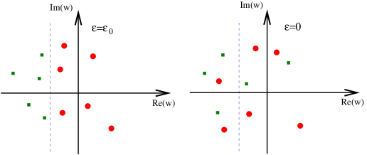
Figure 1: On the left picture, all poles which originate from the same Gamma function are positioned either to the left or to the right of a contour of integration. On the second picture, we take $\epsilon\to 0$, and some of the poles cross to the other side of the contour. To recover a valid representation for the loop-integral, these poles sould be isolated using the Cauchy theorem.

Let us choose a value of $\epsilon$ inside the allowed region and observe the position of the poles with respect to the contours for some $\epsilon$-dependent Gamma functions in our example. The poles of $\Gamma(-1-\epsilon-w_{13})$ and $\Gamma(-1-\epsilon-w_{23})$, at $-1-\epsilon-{\rm Re}(w_{3})+n>{\rm Re}(w_{1})$ and $-1-\epsilon-{\rm Re}(w_{3})+n>{\rm Re}(w_{2})$, are situated to the right of the $w_{1}$ and $w_{2}$ contours, respectively, for all non-negative integers $n$. Let us now take $\epsilon\to 0$. We observe that the first poles, for $n=0$, moved to new positions, $-1-{\rm Re}(w_{3})<{\rm Re}(w_{1})$ and $-1-{\rm Re}(w_{3})<{\rm Re}(w_{2})$, which are on the left side of the contours. The poles for $n>0$ remain on the right side. Therefore, the representation is not valid at $\epsilon\simeq 0$, since the contours separate poles which originate from the same Gamma function. To obtain a valid expression for the integral at $\epsilon=0$, we need to use the Cauchy theorem to isolate the crossing poles ($n=0$).

Smirnov, in Ref. smirnov_book , provides a number of pedagogical examples where this is done. The approach of Smirnov is to deform the multiple contours, using the Cauchy theorem, so that the “offending” poles never cross the contour of integration. Tausk, in Ref. tausk , describes in detail this task as well, using as an explicit example the Mellin-Barnes representation for the two-loop cross box integral. The technique of Tausk is different from the one of Smirnov; the main idea is to account for the poles that end up on the “wrong” side of the contour in a progressive way, as they cross the contours when changing continuously the value of $\epsilon$. In this paper, we have followed the approach of Tausk. We would like to recommend that the interested reader studies the pedagogical example of Ref. tausk . Here we discuss our implementation of the algorithm which is depicted in the flow diagram of Figure 2.

Figure 2: Analytic continuation algorithm

Consider the Mellin-Barnes representation ${\cal R}$ of a loop integral. The integrand of ${\cal R}$ depends initially on Gamma functions. The application of the analytic continuation algorithm requires the iterative evaluation of residues. These may also give rise to Psi functions, which have poles in the same positions the Gamma functions do, and are treated identically for the purposes of analytic continuation. The contours ${\cal C}$ of the representation are straight lines parallel to the imaginary axis, and are chosen so that the real parts of the arguments of all Gamma functions are positive. The same condition determines an allowed region for $\epsilon$, which we will assume that includes the point $\epsilon=\epsilon_{0}$. For the sake of clarity, we will consider the case $\epsilon_{0}<0$, but the method proceeds analogously when $\epsilon_{0}>0$.

The first step is to find the maximum value $\epsilon=\epsilon_{1}$, with $\epsilon_{1}\leq 0$, for which the representation holds. At this value, one or some of the positions of the poles run into a contour. If the set of these poles, ${\cal P}$, is empty, i.e. no poles cross the contours when moving $\epsilon$ from $\epsilon_{0}$ to 0, then the integral can be safely expanded around $\epsilon=0$. So, let us focus on the more interesting case in which ${\cal P}$ is non empty. Here we have to distinguish between $\epsilon_{1}=0$ and $\epsilon_{1}<0$.

If $\epsilon_{1}=0$, at least one pole lies on the contours for the terminating value of $\epsilon$. Then, the representation has an unregulated singularity, and it is not feasible to perform an $\epsilon$ expansion and evaluate the contour integrals numerically. To remedy the situation we must change the contour of integration; we use the Cauchy theorem and displace one or more of the contours parallel to the imaginary axis. Then, we attempt afresh the analytic continuation; the poles should now hit the contour at $\epsilon_{1}<0$. If this does not happen, due to an unfortunate choice of the contour we displaced, we simply iterate the procedure until we succeed.

When $\epsilon_{1}<0$, we have to determine the residues in the poles that cross the contour. If there is only one pole in ${\cal P}$ the situation is simple. Let us look back at the specific example of the one-loop box. By applying the previous steps of the algorithm, we find that the first pole to cross a contour is at $-1-\epsilon-w_{2}-w_{3}=0$. We then choose one of the multiple integrals, e.g. the $w_{2}$ integral, and subtract the residue of the integrand on this pole, at $w_{2}=-1-\epsilon-w_{3}$, to the representation:

$${\cal R}(\epsilon=\epsilon_{0})={\cal R}(\epsilon_{1})-\left.{\rm Res}({\cal R})\right|_{w_{2}=-1-\epsilon-w_{3}}$$ (18)

The residue term in the above expression is a new multiple Mellin-Barnes integral with one integration variable less than in ${\cal R}$. In our example, the pole crosses the $w_{2}$ contour from the right side and we subtract its residue from the original representation. If a pole crosses the contour from the left, we should add its residue. At this point, we have achieved the analytic continuation in $\epsilon$ from $\epsilon_{0}$ to $\epsilon_{1}$. We now repeat the algorithm setting as initial value $\epsilon_{0}=\epsilon_{1}$, and perform the analytic continuation to the next value of $\epsilon$ where a new crossing occurs. We proceed iteratively, until we find all poles which cross the contours of integration in the terms of Eq. 18 and its descendants.

The algorithm is more complicated if many poles cross simultaneously the contour at $\epsilon=\epsilon_{1}$. In our one-loop box example, if we had chosen a symmetric contour ${\cal C}=\left\{{\rm Re}(w_{1})=-0.2,{\rm Re}(w_{2})=-0.2,{\rm Re}(w_{3})=-0.2\right\}$ then we would have two poles crossing at the same time: ${\cal P}=\left\{-1-\epsilon-w_{13}=0,-1-\epsilon-w_{23}=0\right\}$. One way to deal with this situation is to displace the contours in such a way that the degeneracy is removed, i.e. introduce asymmetric contours from the beginning. Another alternative is to take combined residues in all the poles. To correctly account for all the terms in this case, we can imagine that the contours are only slightly displaced from their current position. Then the poles will hit them one at the time and we can take residues successively. Finally, we can restore the original position of the contours without affecting the position of the poles.

There is, however, a caveat in taking multiple residues. Let us consider the case of the one-loop box, where the poles $P_{1}=-1-\epsilon-w_{13}$ and $P_{2}=-1-\epsilon-w_{23}$ hit the contour at the same time. We take residues in sequence, considering first $P_{1}$. We make the “unfortunate” choice to take the residue on the $w_{3}$ integration variable, and not on $w_{1}$. The analytic continuation yields:

$${\cal R}(\epsilon\simeq\epsilon_{0})={\cal R}(\epsilon\simeq\epsilon_{1})-\left.{\rm Res}({\cal R})\right|_{w_{3}=-1-\epsilon-w_{1}}$$

Then we consider the crossing of the $P_{2}$ pole on each of the two terms on the right hand side of the above expression. We find no problems in taking the residue of the first term. However, the position of the $P_{2}$ pole for the second term is now written:

$$P_{2}=\left.1-\epsilon-w_{2}-w_{3}\right|_{w_{3}=-1-\epsilon-w_{1}}=w_{1}-w_{2}.$$

The pole $P_{2}$ is now independent of $\epsilon$ and gets nailed to the contour. This situation is similar to the one we encountered for $\epsilon_{1}=0$, and we can deal with it in exactly the same way by displacing the contours.

We apply the algorithm recursively, to all the terms which are generated by adding the residues of crossing poles to the original parameterization. At the end of this procedure, we obtain a sum of contour integrals plus some terms that do not contain any remaining integral due to taking residues on all integration variables. The method assures that the sum of all these contributions equals the original loop integral when $\epsilon\simeq 0$. So we can expand in a power series of $\epsilon$.

In this Section, we have presented the algorithm assuming that only the dimension parameter $\epsilon$ is required to regulate the Mellin-Barnes parameterization. However, the method proceeds identically for integrals where multiple analytic regulators are required. This could be the case in non-covariant gauges or in integrals with irreducible numerators tausk1 or additional positive powers of propagators veretin .

The actual implementation of the algorithm in a set of routines in both MAPLE and MATHEMATICA is very efficient, and allows to perform the analytic continuation in the regulator parameters in a few seconds, for all the Mellin-Barnes representations that we have studied in this paper.

IV Mellin Barnes representations for tensor integrals

Mellin-Barnes representations, with the exception of the massless two-loop diagonal box topology veretin , have been traditionally employed for the evaluation of master integrals. In this Section, we introduce an efficient generalization of the method to tensor integrals; our method does not require any reduction techniques to master integrals. Common reduction methods produce extremely large algebraic expressions which may also have spurious singular denominators. Here we derive efficient representations for one-loop tensor integrals, which are amenable to numerical integration. We can derive analogous representations for multi-loop integrals by using the re-insertion method of Section II.

We consider a generic one-loop tensor integral of rank $m$ with $n$ external legs:

$$I_{n,m}=\int\frac{d^{d}k}{i\,\pi^{\frac{d}{2}}}\frac{k^{\mu_{1}}\dots k^{\mu_{m}}}{\left[(k+q_{1})^{2}-m_{1}^{2}\right]\left[(k+q_{2})^{2}-m_{2}^{2}\right]\cdots\left[(k+q_{n})^{2}-m_{n}^{2}\right]}\,$$ (19)

where,

$$q_{1}=0,\quad\quad q_{j}=\sum_{i=1}^{j-1}p_{i},$$ (20)

and $p_{i}$ are external incoming momenta. We first introduce Feynman parameters for the denominator. We obtain,

$$I_{n,m}=\Gamma(n)\,\int\frac{d^{d}k}{i\,\pi^{\frac{d}{2}}}\,\int\left(\prod_{i=1}^{n}dx_{i}\right)\,\delta\left(1-\sum_{i=1}^{n}x_{i}\right)\,\frac{k^{\mu_{1}}\dots k^{\mu_{m}}}{\left[(k+P)^{2}-\Delta\right]^{n}}\,,$$ (21)

where

$$P=\sum_{i=1}^{n}x_{i}q_{i},$$ (22)

and

$$\Delta=\sum_{i=1}^{n}x_{i}m_{i}^{2}+\sum_{j=2}^{n}\sum_{i<j}x_{i}x_{j}\left[-\left(q_{i}-q_{j}\right)^{2}\right]$$ (23)

Now we perform the usual shift in the loop momentum, $k=K-P$, and we obtain,

$$I_{n,m}=\Gamma(n)\,\,\int\left(\prod_{i=1}^{n}dx_{i}\right)\,\delta\left(1-\sum_{i=1}^{n}x_{i}\right)\,\sum_{r\leq m}\int\frac{d^{d}K}{i\,\pi^{\frac{d}{2}}}\frac{\left\{K^{r}P^{m-r}\right\}^{[\mu_{1},\ldots,\mu_{m}]}}{(K^{2}-\Delta)^{n}}\,,$$ (24)

where, we denote

$$\left\{K^{r}P^{m-r}\right\}^{[\mu_{1},\ldots,\mu_{m}]}=\sum_{\{j_{1},\ldots,j_{m}\}}K^{\mu_{j_{1}}}\cdots K^{\mu_{j_{r}}}P^{\mu_{j_{r+1}}}\cdots P^{\mu_{j_{m}}},$$ (25)

$$\hskip 56.9055pt\{j_{1},\ldots,j_{m}\}\in\mbox{permutations}(1,\ldots,m).$$

We find the standard Feynman representation for the generic tensor one-loop $n$-point function, by integrating the loop momentum:

$$I_{n,m} = (-1)^{n}\int\left(\prod_{i=1}^{n}dx_{i}\right)\,\delta\left(1-\sum_{i=1}^{n}x_{i}\right)\,\frac{1}{{\Delta^{n-\frac{d}{2}}}}$$ (26)

$$\times\sum_{r\leq m}\,\frac{\Gamma\left(n-\frac{d}{2}-\frac{r}{2}\right)}{2^{\frac{r}{2}}}\left\{{\cal A}_{r}P^{m-r}\right\}^{[\mu_{1},\ldots,\mu_{m}]}\Delta^{\frac{r}{2}},\,$$

where ${\cal A}_{r}=0$ for $r$ odd, and ${\cal A}_{r}=g^{\left[\mu_{1}\mu_{2}\right.}\cdots g^{\left.\mu_{r-1}\mu_{r}\right]}$ for $r$ even. We observe that the sum, in the second line of the equation, is a polynomial in the Feynman parameters, with tensor coefficients:

$$\sum_{r\leq m}\,\frac{\Gamma\left(n-\frac{d}{2}-\frac{r}{2}\right)}{2^{\frac{r}{2}}}\left\{{\cal A}_{r}P^{m-r}\right\}^{[\mu_{1},\ldots,\mu_{m}]}\Delta^{\frac{r}{2}}=\sum_{\{\nu_{i}>0\}}C(\{\nu_{i}\};\{p_{i}^{\mu_{j}}\})x_{1}^{\nu_{1}-1}\cdots x_{n}^{\nu_{n}-1}$$ (27)

For the scalar integral with unit powers of propagators, this sum is $\Gamma(n-\frac{d}{2})$.

We will use Eq. 26 to derive Mellin-Barnes representations for the tensor loop-integral. We would like to exploit the fact that the Feynman representation of the scalar and tensor integrals have the same denominator:

$$\frac{1}{\Delta^{n-\frac{d}{2}}}.$$

In Section II, we have seen that we can obtain a Mellin-Barnes representation for a loop integral by decomposing the denominator of the Feynman parameterization with Eq. 5. We should anticipate that the Mellin-Barnes representations of tensors and scalars are, therefore, very similar. We can verify this intuition, if we consider one generic term in the polynomial of Eq. 27, and follow the steps of Section II. Decomposing the denominator with Eq. 5, we obtain

$$\frac{x_{1}^{\nu_{1}-1}\cdots x_{n}^{\nu_{n}-1}}{\Delta^{n-\frac{d}{2}}}\to x_{1}^{\nu_{1}-1}\cdots x_{n}^{\nu_{n}-1}$$

$$(-s_{\alpha})^{\frac{d}{2}-n}\int\left(\prod_{i=1}^{\alpha-1}dw_{i}\Gamma(-w_{i})(-s_{i})^{w_{i}}(-s_{\alpha})^{-w_{i}}\right)\Gamma(n-\frac{d}{2}+w_{12\ldots{(\alpha-1)}})\,x_{1}^{\beta_{1}(\vec{w})}\cdots x_{n}^{\beta_{n}(\vec{w})}$$ (28)

where $\alpha$ is the number of kinematic scales $s_{i}$ in the integral. The factors $x_{i}^{\beta_{i}(\vec{w})}$ are universal for all terms in Eq. 27, and originate from the dependence of $\Delta$ on the Feynman parameters. We now proceed to integrate out the Feynman parameters using Eq. 7. This integration yields Gamma functions

$$x_{i}^{\beta_{i}(\vec{w})+\nu_{i}-1}\stackrel{{\scriptstyle\int dx_{i}}}{{\longrightarrow}}\Gamma(\beta_{i}+\nu_{i})=\Gamma(1+\beta_{i})(1+\beta_{i})(2+\beta_{i})\cdots(\nu_{i}-1+\beta_{i})$$ (29)

Rewriting all Gamma functions as above in Eq. 27, we obtain, for the tensor integral, the Gamma functions of the scalar integral multiplied by simple factors with Mellin-Barnes integration variables.

The result for the one-loop tensor integrals depends on the topology and the rank of the tensors in a rather complicated manner. However, we find that the representation is of the following form

$$I_{n,m} = \frac{(-s_{\alpha})^{\frac{d}{2}-n}}{(2\pi i)^{\alpha-1}}\int\left(\prod_{i=1}^{\alpha-1}dw_{i}\Gamma(-w_{i})(-s_{i})^{w_{i}}(-s_{\alpha})^{(-w_{i})}\right)\Gamma^{(scalar)}(w_{i},\ldots,w_{\alpha-1})$$ (30)

$$\hskip 142.26378pt\times h^{(m)}(w_{1},\ldots,w_{\alpha-1}),$$

The first line of the above representation contains all the terms which already appear in the analogous representation of the scalar integral with unit powers of propagators. The function $h^{(m)}$ is a polynomial in the Mellin-Barnes variables, with tensor coefficients in terms of the external momenta. This is very important for our strategy to evaluate tensor integrals and Feynman diagrams. The polynomial in the numerator is smooth, and it does not affect the analytic continuation in $\epsilon$. We can therefore perform the continuation collectively for all tensor integrals and diagrams of the same topology.

We organize the evaluation of tensor integrals and diagrams of a topology as follows. We first find the Mellin-Barnes parameterization of the scalar integral of the topology, and multiply the integrand with a template function $h(\{w_{i}\})$ which we assume depends on all Mellin-Barnes variables. Then, we apply the analytic continuation algorithm of Section III keeping $h$ general. We expand in $\epsilon$, and create numerical programs for the evaluation of the expansion for any smooth function $h$. This part of the evaluation needs to be performed only once for a given topology. Then we must identify the polynomial for the evaluation of the specific tensors or diagrams that we are interested in. We have written FORM form and MATHEMATICA programs which perform the steps that we described in this Section, and derive the explicit functional form of the polynomials in Eq. 30. We then write numerical routines for their evaluation, and link them to the general routines for the $\epsilon$ expansion of the integrals of the topology.

This approach is efficient for the application of our technique to tensor integrals. It turns out, however, that the expressions for the polynomials are quite long for high rank tensors. We have observed that we can reduce the size of the expressions substantially with a simple modification. The terms $\Delta^{\frac{r}{2}}$ in Eq. 26 are lengthy, and when we integrate out the Feynman parameters they give rise to large expressions in $h^{(m)}$ of Eq. 30. We rewrite Eq. 26 in a different way,

$$I_{n,m} = (-1)^{n}\int\left(\prod_{i=1}^{n}dx_{i}\right)\,\delta\left(1-\sum_{i=1}^{n}x_{i}\right)\,$$ (31)

$$\times\sum_{r\leq m}\,\frac{\Gamma\left(n-\frac{d}{2}-\frac{r}{2}\right)}{2^{\frac{r}{2}}}\frac{1}{{\Delta^{n-\frac{d+r}{2}}}}\left\{{\cal A}_{r}P^{m-r}\right\}^{[\mu_{1},\ldots,\mu_{m}]}\,$$

Then, we introduce a Mellin-Barnes decomposition for each denominator:

$$\frac{1}{\Delta^{n-\frac{r+d}{2}}},$$

and integrate out the Feynman parameters. At the end of this procedure, we obtain a sum of $\left[\frac{m}{2}\right]+1$ Mellin-Barnes integrals for a tensor of rank $m$. All integrals correspond to the Mellin-Barnes representation of the scalar integral with shifted dimension $d\to d+r$. Each of them has a different polynomial $h^{(m)}_{r}$ in the numerator. However, these are substantially shorter than the polynomial $h^{(m)}$ in Eq. 30.

It is worth to note that, with our method, we never introduce spurious singularities. The evaluation of the higher rank tensors and diagrams in gauge theories is very efficient, since we never require the manipulation of lengthy expressions. The polynomials $h^{(m)}_{r}$ can be large, however, they require a minimum amount of handling before generating numerical codes for their evaluation.

Here we have presented the derivation of efficient representations for one-loop integrals. The method may be applied to multi-loop integrals using the one-loop tensor integral representations as building blocks. The analogous functions of $h^{(m)}_{r}$ in multi-loop tensors contain Gamma functions in the denominator. However, they are smooth and maintain the properties which are required for a collective evaluation of all tensors of a topology. Explicit applications with multi-loop tensor integrals will be examined in future work.

V Numerical evaluation of Mellin-Barnes representations

After analytic continuation, the contour integrals can be safely expanded in power series of $\epsilon$. The coefficients of the expansion are also contour integrals which, in general, contain in their integrand Gamma functions, Gamma function derivatives, simple logarithms, and powers of the kinematic parameters. In earlier works, these integrals were computed analytically. The standard approach is to evaluate them by means of the residue theorem, i.e. summing an infinite number of residues and expressing the power series as logarithms, polylogarithms and harmonic polylogarithms.

This method is cumbersome for the evaluation of integrals with more than one Mellin-Barnes variable. In all cases presented in the literature, integrals with more than one dimension are reduced to one-dimensional integrals with a variety of clever, however not general, tricks. Typical procedures include direct integration in simple situations, the application of Barnes lemmas smirnov ; tausk ; smirnov_book , and the expansion in Laurent series around an integer value of one of the variables. In a few cases, a careful inspection of the multi-dimensional integrals reveals exact cancellations between different components which yield significant simplifications.

Many integrals which are relevant for physical applications, such as the massless double box with two external legs off-shell and one-loop tensor integrals with six external legs, after the analytic continuation in $\epsilon$, are expressed in terms of hundreds of Mellin-Barnes components; some of them have a very high dimensionality. The analytic methods are not suitable for such problems. In our method, we choose to evaluate the MB integrals numerically by direct integration over the contours.

The procedure we follow is, conceptually, straightforward. In practice, the implementation of the numerical evaluation requires a significant work in automating the book-keeping of the various terms. Tensor integrals require significantly more complex book-keeping due to large expressions that multiply the Gamma functions in the integrand of their Mellin-Barnes representation. Our computer programs are organized in the following way. We first use MAPLE, FORM form , and MATHEMATICA routines to derive Mellin-Barnes representations for the integrals that we need to compute. We then perform the analytic continuation of Section III, and we expand the integrands in powers of $\epsilon$ using MAPLE and MATHEMATICA. As the next step, we translate the integrands into FORTRAN routines which evaluate them as complex quantities.

There are many options to calculate numerically the sum of the Mellin-Barnes integrals which emerge from the routines for the $\epsilon$ expansion. For example, we can combine all contributions in a single common integrand, so that large numerical cancellations take place before integration. However, the finding of the peaks and the adaptation of the integration routines become less efficient. Following a diametric approach, we could integrate all components separately and compute their sum at the end. Then, the adaptation of the numerical integration is optimal, however, the numerical precision is sensitive to cancellations. In practice, we follow a hybrid approach and group together integrals with equivalent contours. We have achieved a reasonable efficiency and speed for all the computations that we present in this paper. Since we aim to keep our integration method general, we do not attempt any special simplifications by, for example, applying Barnes lemmas or exploiting symmetries of particular contours.

For the numerical integration, we maintain the contours as straight lines parallel to the imaginary axis. We map them onto a real interval with a simple transformation,

$$\frac{1}{2\pi i}\int_{c-i\infty}^{c+i\infty}dwf(w)=\frac{1}{2\pi}\int_{0}^{1}\frac{d\lambda}{\lambda(1-\lambda)}f\left(c-i\ln\left(\frac{\lambda}{1-\lambda}\right)\right)$$ (32)

In all cases that we have considered, the integrands vanish rapidly when the integration variables take values away from the real line $(\lambda\simeq\frac{1}{2})$. The Mellin-Barnes integrals do not present problematic numerical instabilities, and converge rather fast. We perform the multidimensional integrations using the Cuhre and Vegas routines of the CUBA library cuba . To gain some speed, we integrate the real and imaginary parts of the integrals concurrently, using the same grid. The grid is adapted to the peaks of the real part, however, the quality of the integration for the imaginary part is only mildly affected. On the other hand, there is another subtle point concerning the convergence of the imaginary parts. As they always start an order later in the expansion in $\epsilon$, the analytic expressions for them would be simpler than the corresponding real ones. When integrating numerically this relative simplicity is reflected by a faster convergence when compared to the real pieces at the same order.

The numerical results depend on the values for the kinematic scales of the integrals. With our approach, we use the same expressions for the evaluation of the integrals in all kinematic regions. As we explained earlier, the only analytic continuations in kinematic variables that we must perform, is for simple functions of the type $(-s_{ij})^{z}$ and $\log(-s_{ij})$. These are implemented trivially, in a branched format, in numerical programs. In this paper, we present multi-loop integrals for fixed kinematic parameters. However, we have arranged our routines so that a numerical integration over the phase-space can be performed simultaneously with the Mellin-Barnes integrations.

A problematic case for our numerical algorithms is the evaluation of loop integrals with massive internal propagators in non-Euclidean kinematic regions. Typically, Mellin-Barnes represenations for such integrals exhibit a very slow damping at $\pm i\infty$ in physical regions. The mapping of the integration region to a finite interval that we have considered in Eq. 32 is not adequate, and contour deformations together with more sophisticated algorithms for the evaluation of oscillatory integrals are required. We defer the study of such situations for a future project.

We have achieved a full automatization of the code generation for the numerical evaluation. This has allowed us to apply our method to diverse problems. Our approach can be improved and refined further in the future by considering, for example, a clever analysis of the terms before integration in order to avoid numerical cancellations or more sophisticated mappings which can smoothen the peak structure of the integrands. However, as we will see in the rest of the paper, our first, naive, implementation is already sufficient to obtain accurate results for complicated integrals in a reasonable time.

In what follows we present results for one, two, and three loop integrals. Some of the integrals are known analytically, and we use them to verify our numerical programs. We also present new loop integrals, which would be extremely tedious to calculate with traditional methods.

VI Results

In this Section we present results for one, two, and three-loop integrals that we obtain with our method. For each integral, we present the coefficients of its expansion in $\epsilon=2-\frac{d}{2}$ through the finite term:

$${\cal I}=\int\left(\prod_{i}\frac{d^{d}k_{i}}{i\pi^{\frac{d}{2}}}\right)\frac{\{k_{i}^{\mu}\}}{\prod_{j}{{\rm propagator}}_{j}}=\sum_{i=0}^{r}\,c_{i}\,\epsilon^{-i}\,,$$ (33)

where $r$ is the depth of the leading pole in $\epsilon$. We estimate the errors associated with our results for $c_{i}$, by adding, in quadrature, the integration errors of all contributions from the residue decomposition.

VI.1 One loop hexagon: the scalar integral

The first integral we consider is the massless one-loop hexagon, depicted in Figure 3.

Figure 3: The hexagon topology

For massless external legs, we derive an eight-dimensional Mellin-Barnes representation for this integral. Due to the high dimensionality, the analytic continuation in $\epsilon$ involves the crossing of the contours of integration from many poles, and the Mellin-Barnes expression after the continuation consists of about two hundred terms. This example demonstrates the advantage of the automatic algorithm we described in Section III, since the book-keeping is done automatically and our routines perform the $\epsilon$ expansion in fractions of a minute.

After the analytic continuation and the expansion in series of $\epsilon$, only integrals with low dimensionality contribute to the poles and finite pieces of the series. The integration over Feynman parameters produces a denominator factor $1/\Gamma(-2\epsilon)$, which contributes factors of $\epsilon$ in the series expansion. The eight-dimensional component, in which no residues have been taken, drops out from the finite part. In addition, most of the residues in the analytic continuation do not give rise to poles in $\epsilon$; a few components only develop a singularity that compensates the $\epsilon$ in the overall factor. For the scalar hexagon, we find integrals with up to three dimensions which contribute to the poles and the finite term. This mechanism, which reduces the dimensionality of the representation in the leading coefficients of the $\epsilon$ expansion, is not specific to the hexagon topology, but is typical of Mellin-Barnes representations of scalar multi-leg integrals.

In Table 2 we present explicit results for the scalar hexagon in phase space points corresponding to the physical region for the $2\rightarrow 4$ process. To check the efficiency of our integration routines in all the phase-space, we have sampled hundreds of points. Here, we only show representative results in the phase-space points of Table 1. These points were generated starting from explicit values for the momenta in four dimensions, so they have a vanishing Gram determinant.

point	$s_{12}$	$s_{23}$	$s_{34}$	$s_{45}$	$s_{56}$	$s_{16}$	$s_{123}$	$s_{234}$	$s_{345}$
$P_{1}$	1	-0.232033	0.096793	0.025066	0.465569	-0.015783	0.63356	-0.219996	0.336498
$P_{2}$	1	-0.056339	0.054104	0.111985	0.583564	-0.038557	0.74554	-0.191061	0.260063
$P_{3}$	1	-0.336912	0.099306	0.228826	0.333228	-0.086216	0.64116	-0.286003	0.580452
$P_{4}$	1	-0.310819	0.012151	0.020687	0.561466	-0.349136	0.58216	-0.318051	0.114844
$P_{5}$	1	-0.07491	0.048452	0.279727	0.314164	-0.426813	0.73852	-0.449749	0.532752
$P_{6}$	1	-0.447378	0.10597	0.052091	0.277082	-0.484988	0.32942	-0.400468	0.170418
$P_{7}$	1	-0.081759	0.143257	0.139358	0.183411	-0.544412	0.81512	-0.361942	0.31596
$P_{8}$	1	-0.115263	0.054869	0.154172	0.209043	-0.569659	0.63722	-0.477605	0.410718
$P_{9}$	1	-0.331123	0.011523	0.033009	0.252287	-0.635452	0.38202	-0.441643	0.309497
$P_{10}$	1	-0.297484	0.010637	0.05663	0.345614	-0.88129	0.68562	-0.541753	0.083132

Table 1: Explicit values of the invariants for some of the phase space points used for the evaluation of the hexagon topology. The points correspond to the physical region of the $2\rightarrow 4$ scattering of massless particles.

As can be seen from Table 2, our method is perfectly capable of evaluating multi-scale integrals, such as the scalar hexagon, reliably in all phase-space. The results in the Table correspond to a fixed number of evaluations, thus the difference in the relative errors for different points. It took a couple of minutes per point on a 2.8GHZ CPU to evaluate them.

Point	$c_{2}$	$c_{1}$	$c_{0}$
$P_{1}$	$$\begin{array}[]{lr@{.}lc}-&24550&802400&(0)\\ +&i\cdot 0&000000&(0)\end{array}$$	$$\begin{array}[]{lr@{.}lc}-&129377&216040&(5)\\ -&i\cdot 69329&856499&(5)\end{array}$$	$$\begin{array}[]{lr@{.}lc}-&249435&&(40.)\\ -&i\cdot 365517&9&(3)\end{array}$$
$P_{2}$	$$\begin{array}[]{lr@{.}lc}-&10666&332700&(0)\\ +&i\cdot 0&000000&(0)\end{array}$$	$$\begin{array}[]{lr@{.}lc}-&42307&989040&(3)\\ -&i\cdot 18370&333000&(3)\end{array}$$	$$\begin{array}[]{lr@{.}lc}-&34595&&(66.)\\ -&i\cdot 53139&1&(8)\end{array}$$
$P_{3}$	$$\begin{array}[]{lr@{.}lc}-&1153&682480&(0)\\ +&i\cdot 0&000000&(0)\end{array}$$	$$\begin{array}[]{lr@{.}lc}-&3091&953473&(3)\\ -&i\cdot 2868&081530&(4)\end{array}$$	$$\begin{array}[]{lr@{.}lc}&2292&&(2.)\\ -&i\cdot 6531&15&(6)\end{array}$$
$P_{4}$	$$\begin{array}[]{lr@{.}lc}-&48753&897600&(0)\\ +&i\cdot 0&000000&(0)\end{array}$$	$$\begin{array}[]{lr@{.}lc}-&256890&405260&(4)\\ -&i\cdot 152982&841000&(4)\end{array}$$	$$\begin{array}[]{lr@{.}lc}-&432690&&(5.)\\ -&i\cdot 806442&61&(4)\end{array}$$
$P_{5}$	$$\begin{array}[]{lr@{.}lc}-&2502&711680&(0)\\ +&i\cdot 0&000000&(0)\end{array}$$	$$\begin{array}[]{lr@{.}lc}-&10214&467200&(2)\\ -&i\cdot 7425&550140&(3)\end{array}$$	$$\begin{array}[]{lr@{.}lc}-&8934&&(16.)\\ -&i\cdot 30275&25&(6)\end{array}$$
$P_{6}$	$$\begin{array}[]{lr@{.}lc}-&3857&953670&(0)\\ +&i\cdot 0&000000&(0)\end{array}$$	$$\begin{array}[]{lr@{.}lc}-&11372&775324&(2)\\ -&i\cdot 12047&807600&(3)\end{array}$$	$$\begin{array}[]{lr@{.}lc}&6715&7&(9)\\ -&i\cdot 35512&41&(2)\end{array}$$
$P_{7}$	$$\begin{array}[]{lr@{.}lc}-&2078&190700&(0)\\ +&i\cdot 0&000000&(0)\end{array}$$	$$\begin{array}[]{lr@{.}lc}-&6541&063310&(1)\\ -&i\cdot 6138&816950&(2)\end{array}$$	$$\begin{array}[]{lr@{.}lc}&1413&&(2.)\\ -&i\cdot 18965&48&(6)\end{array}$$
$P_{8}$	$$\begin{array}[]{lr@{.}lc}-&3356&184660&(0)\\ +&i\cdot 0&000000&(0)\end{array}$$	$$\begin{array}[]{lr@{.}lc}-&13032&698020&(3)\\ -&i\cdot 10343&407301&(2)\end{array}$$	$$\begin{array}[]{lr@{.}lc}-&8558&&(6.)\\ -&i\cdot 40209&00&(3)\end{array}$$
$P_{9}$	$$\begin{array}[]{lr@{.}lc}-&45864&213500&(0)\\ +&i\cdot 0&000000&(0)\end{array}$$	$$\begin{array}[]{lr@{.}lc}-&281098&336280&(4)\\ -&i\cdot 144019&061999&(3)\end{array}$$	$$\begin{array}[]{lr@{.}lc}-&649614&&(5.)\\ -&i\cdot 882892&34&(2)\end{array}$$
$P_{10}$	$$\begin{array}[]{lr@{.}lc}-&21516&252000&(0)\\ +&i\cdot 0&000000&(0)\end{array}$$	$$\begin{array}[]{lr@{.}lc}-&97739&299610&(3)\\ -&i\cdot 67551&061100&(3)\end{array}$$	$$\begin{array}[]{lr@{.}lc}-&99008&&(13.)\\ -&i\cdot 306919&34&(2)\end{array}$$

Table 2: The scalar massless hexagon evaluated in some physical points of the phase space. The errors of the numerical integration are quoted in parenthesis, and they affect the last figure/s respectively.

VI.2 One-loop hexagon: tensor integrals

The most severe problem in evaluating multi-leg amplitudes, is the appearance of tensor numerators in the loop integrals. Our method, provides a powerful tool for their evaluation. The scalar hexagon, which we discussed before, provided a nice test-ground for the analytic continuation algorithm and the numerical integration strategy. Here, we consider tensor integrals for the same topology, in order to demonstrate the potential of the method for computing realistic quantities that arise in gauge theories.

Using the procedure described in Section IV, we perform the analytic continuation for an arbitrary tensor. At variance with the scalar case, now we find components with more than three MB variables contributing to the finite pieces in $\epsilon$. For instance, for a typical rank three tensor, integrals with all eight Mellin-Barnes variables are required. This calculation provides stringent tests on our implementation, due to the complex book-keeping of the tensorial terms in the Mellin-Barnes representations, and the efficiency of our routines to evaluate the integrals with high dimensionality.

In Table 3 we show results for tensors up to rank 6 evaluated in a symmetric point $\{s_{ij}=s_{ijk}=-1\}$ in the Euclidean region. For these examples, we contracted all the loop momenta in the numerator with the same external momentum. All such tensor contractions, with odd rank, should vanish; we reproduce this result. On the table, we also show results obtained by reducing the tensors using the program AIR air . We were not able to reduce the high rank tensors to master integrals in a closed analytic form. The reduction was only possible by substituting the kinematic invariants to their numerical value at this particular phase-space point before solving the system of IBP equations. We have also made additional comparisons with the reduction method, for other tensor contractions and a different point inside the physical region.

Tensor	MB	AIR
$q_{2}\cdot k$	$$\begin{array}[]{@{(}r@{.}lcc@{\,i\cdot}r@{.}lc@{)}r}0&000000&(0)&+&0&000000&(0)&\epsilon^{-2}+\\ 0&00000&(1)&+&0&00000&(1)&\epsilon^{-1}+\\ 0&000&(2)&+&0&00000&(1)&\end{array}$$	0
$q_{2}\cdot k\,q_{2}\cdot k$	$$\begin{array}[]{@{(}r@{.}lcc@{\,i\cdot}r@{.}lc@{)}r}0&500000&(0)&+&0&000000&(0)&\epsilon^{-2}+\\ 0&71139&(1)&+&0&00000&(1)&\epsilon^{-1}+\\ 0&0947&(8)&+&0&00000&(1)&\\ \end{array}$$	$$\begin{array}[]{r@{.}lr}0&5&\epsilon^{-2}+\\ 0&711392&\epsilon^{-1}+\\ 0&094845&\end{array}$$
$q_{2}\cdot k\,q_{2}\cdot k\,q_{2}\cdot k$	$$\begin{array}[]{@{(}r@{.}lcc@{\,i\cdot}r@{.}lc@{)}r}0&000000&(0)&+&0&000000&(0)&\epsilon^{-2}+\\ 0&0000&(1)&+&0&00000&(1)&\epsilon^{-1}+\\ 0&00&(2)&+&0&02&(2)&\end{array}$$	0
$q_{2}\cdot k\,q_{2}\cdot k\,q_{2}\cdot k\,q_{2}\cdot k$	$$\begin{array}[]{@{(}r@{.}lcc@{\,i\cdot}r@{.}lc@{)}r}0&125000&(0)&+&0&000000&(0)&\epsilon^{-2}+\\ 0&3861&(1)&+&0&00000&(1)&\epsilon^{-1}+\\ 0&65&(3)&+&0&02&(3)&\end{array}$$	$$\begin{array}[]{r@{.}lr}0&125&\epsilon^{-2}-\\ 0&386181&\epsilon^{-1}+\\ 0&65996&\end{array}$$
$q_{2}\cdot k\,q_{2}\cdot k\,q_{2}\cdot k\,q_{2}\cdot k\,q_{2}\cdot k$	$$\begin{array}[]{@{(}r@{.}lcc@{\,i\cdot}r@{.}lc@{)}r}0&000000&(0)&+&0&000000&(0)&\epsilon^{-2}+\\ 0&00000&(9)&+&0&00000&(1)&\epsilon^{-1}+\\ 0&04&(4)&-&0&02&(4)&\end{array}$$	0
$q_{2}\cdot k\,q_{2}\cdot k\,q_{2}\cdot k\,q_{2}\cdot k\,q_{2}\cdot k\,q_{2}\cdot k$	$$\begin{array}[]{@{(}r@{.}lcc@{\,i\cdot}r@{.}lc@{)}r}0&031250&(0)&+&0&000000&(0)&\epsilon^{-2}+\\ 0&12466&(6)&+&0&00000&(1)&\epsilon^{-1}+\\ 0&27&(1)&-&0&00&(1)&\end{array}$$	$$\begin{array}[]{r@{.}lr}0&03125&\epsilon^{-2}-\\ 0&1246703&\epsilon^{-1}+\\ 0&279587&\end{array}$$

Table 3: Contracted tensors evaluated in a symmetric point in the Euclidean region. We compare with results obtained with the program AIR.

As in the scalar case, we sampled several phase space points in the physical region, calculating a variety of contracted tensors at each rank. In Table 4 we list the cases we considered, and in Table 5 we show explicit results for the contraction $q_{2}\cdot k\,q_{2}\cdot k\,q_{3}\cdot k\,q_{4}\cdot k\,q_{5}\cdot k\,q_{6}\cdot k\,$ in the same phase space points that we considered for the scalar hexagon. We find that our routines perform extremely well, including the highest rank cases that we considered here.

Rank	Contraction
1	$q_{2}\cdot k$
2	$q_{2}\cdot k\,q_{4}\cdot k$ $q_{2}\cdot k\,q_{5}\cdot k$
3	$q_{2}\cdot k\,q_{2}\cdot k\,q_{4}\cdot k$ $q_{2}\cdot k\,q_{4}\cdot k\,q_{5}\cdot k$
4	$q_{2}\cdot k\,q_{2}\cdot k\,q_{3}\cdot k\,q_{4}\cdot k$ $q_{2}\cdot k\,q_{4}\cdot k\,q_{5}\cdot k\,q_{6}\cdot k$ $q_{2}\cdot k\,q_{3}\cdot k\,q_{5}\cdot k\,q_{6}\cdot k$
5	$q_{2}\cdot k\,q_{3}\cdot k\,q_{4}\cdot k\,q_{5}\cdot k\,q_{6}\cdot k$ $q_{2}\cdot k\,q_{2}\cdot k\,q_{4}\cdot k\,q_{6}\cdot k\,q_{6}\cdot k$ $k\cdot k\,q_{2}\cdot k\,q_{3}\cdot k\,q_{4}\cdot k$
6	$q_{2}\cdot k\,q_{2}\cdot k\,q_{3}\cdot k\,q_{4}\cdot k\,q_{5}\cdot k\,q_{6}\cdot k$ $k\cdot k\,q_{2}\cdot k\,q_{3}\cdot k\,q_{4}\cdot k\,q_{5}\cdot k$ $k\cdot k\,k\cdot k\,k\cdot k$

Table 4: Tensor contractions evaluated for the hexagon topology

Point	$c_{2}$	$c_{1}$	$c_{0}$
$P_{1}$	$$\begin{array}[]{lr@{.}lc}-&402&790580&(0)\\ +&i\cdot 0&000000&(0)\end{array}$$	$$\begin{array}[]{lr@{.}lc}-&1919&50&(1)\\ -&i\cdot 1248&33&(2)\end{array}$$	$$\begin{array}[]{lr@{.}lc}-&3019&&(55.)\\ -&i\cdot 6068&&(50.)\end{array}$$
$P_{2}$	$$\begin{array}[]{lr@{.}lc}-&253&831615&(0)\\ +&i\cdot 0&000000&(0)\end{array}$$	$$\begin{array}[]{lr@{.}lc}-&876&7&(2)\\ -&i\cdot 676&4&(1)\end{array}$$	$$\begin{array}[]{lr@{.}lc}-&538&&(56.)\\ -&i\cdot 2440&&(50.)\end{array}$$
$P_{3}$	$$\begin{array}[]{lr@{.}lc}-&47&453378&(0)\\ +&i\cdot 0&000000&(0)\end{array}$$	$$\begin{array}[]{lr@{.}lc}-&149&099&(6)\\ -&i\cdot 145&128&(4)\end{array}$$	$$\begin{array}[]{lr@{.}lc}-&79&&(2.)\\ -&i\cdot 485&&(2.)\end{array}$$
$P_{4}$	$$\begin{array}[]{lr@{.}lc}-&3876&804240&(0)\\ +&i\cdot 0&000000&(0)\end{array}$$	$$\begin{array}[]{lr@{.}lc}-&23083&200&(2)\\ -&i\cdot 12161&074&(2)\end{array}$$	$$\begin{array}[]{lr@{.}lc}-&53835&&(6.)\\ -&i\cdot 72507&&(5.)\end{array}$$
$P_{5}$	$$\begin{array}[]{lr@{.}lc}-&52&452711&(0)\\ +&i\cdot 0&000000&(0)\end{array}$$	$$\begin{array}[]{lr@{.}lc}-&214&000&(2)\\ -&i\cdot 158&220&(2)\end{array}$$	$$\begin{array}[]{lr@{.}lc}-&214&&(2.)\\ -&i\cdot 663&&(1.)\end{array}$$
$P_{6}$	$$\begin{array}[]{lr@{.}lc}-&224&589492&(0)\\ +&i\cdot 0&000000&(0)\end{array}$$	$$\begin{array}[]{lr@{.}lc}-&887&7120&(5)\\ -&i\cdot 701&8064&(5)\end{array}$$	$$\begin{array}[]{lr@{.}lc}-&888&&(1.)\\ -&i\cdot 2796&9&(9)\end{array}$$
$P_{7}$	$$\begin{array}[]{lr@{.}lc}-&54&532983&(0)\\ +&i\cdot 0&000000&(0)\end{array}$$	$$\begin{array}[]{lr@{.}lc}-&172&177&(4)\\ -&i\cdot 161&007&(7)\end{array}$$	$$\begin{array}[]{lr@{.}lc}-&26&&(2.)\\ -&i\cdot 531&&(2.)\end{array}$$
$P_{8}$	$$\begin{array}[]{lr@{.}lc}-&47&254266&(0)\\ +&i\cdot 0&000000&(0)\end{array}$$	$$\begin{array}[]{lr@{.}lc}-&179&409&(1)\\ -&i\cdot 143&862&(2)\end{array}$$	$$\begin{array}[]{lr@{.}lc}-&127&&(1.)\\ -&i\cdot 558&&(1.)\end{array}$$
$P_{9}$	$$\begin{array}[]{lr@{.}lc}-&865&507076&(0)\\ +&i\cdot 0&000000&(0)\end{array}$$	$$\begin{array}[]{lr@{.}lc}-&5612&7500&(2)\\ -&i\cdot 2716&2898&(1)\end{array}$$	$$\begin{array}[]{lr@{.}lc}-&15300&&(2.)\\ -&i\cdot 17634&&(1.)\end{array}$$
$P_{10}$	$$\begin{array}[]{lr@{.}lc}-&1318&087970&(0)\\ +&i\cdot 0&000000&(0)\end{array}$$	$$\begin{array}[]{lr@{.}lc}-&6160&7460&(9)\\ -&i\cdot 4137&4238&(2)\end{array}$$	$$\begin{array}[]{lr@{.}lc}-&7611&&(2.)\\ -&i\cdot 19356&&(2.)\end{array}$$

Table 5: Results for the rank six tensor $q_{2}\cdot k\,q_{2}\cdot k\,q_{3}\cdot k\,q_{4}\cdot k\,q_{5}\cdot k\,q_{6}\cdot k\,$ for the hexagon topology at one loop. The phase space points are detailed in Table 1

We should note that, due to the way that we organize the evaluation of the tensors in Section IV, we do not anticipate that the evaluation of Feynman graphs, such as the ones in the one-loop six photon amplitude, are significantly harder than the six rank tensors that we presented. In addition, our routines allow a combined integration over the Mellin-Barnes variables and the kinematic invariants.

VI.3 On-shell planar double box

Figure 4: The massless double box.

We now compute two-loop integrals, and we consider first the massless planar double box with on-shell legs shown in Fig. 4. This integral is known analytically in Ref. smirnov . As discussed in Section II, it can be expressed as a MB contour integral in four complex dimensions. Performing the analytic continuation in $\epsilon$, we get terms where residues in all the variables have been taken (i.e. terms without any contour integral left); these contain poles through $1/\epsilon^{4}$. The terms through ${\cal O}(\epsilon^{0})$ require Mellin-Barnes integrals with one and two integration variables.

In Figure 5 we show our results for the finite pieces of the on-shell double box in the physical region for the $p_{1}+p_{2}\rightarrow p_{3}+p_{4}$ process depicted in Figure 4. We set $s=(p_{1}+p_{2})^{2}=1$, and plot, as functions of $t=(p_{2}-p_{3})^{2}$, the finite term $c_{0}$ and the comparison of our numerical calculation to the analytic result of smirnov .

As can be seen from the figure, it is possible to achieve an accuracy of a few parts in ten thousand, in a few seconds per phase-space point. The bigger error band for the imaginary part, reflects our naive strategy to integrate both real and imaginary part with the same grid. The coefficients for the simple and double poles in $\epsilon$, not shown in the figure, agree with the analytic calculation with even better accuracy, whereas the cubic and quartic poles are analytic expressions also in our case (as they do not involve any MB integration) and coincide with the ones in smirnov .

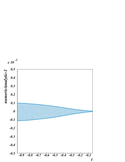
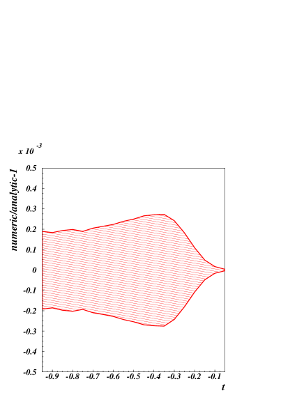
Figure 5: Results for the finite part of the planar double box in the physical region for a $2\rightarrow 2$ process. On the two left panels we plot the real and imaginary parts (upper and lower plots respectively) of the finite term as a function of $t$ for fixed value of $s=1$. The estimated error of the numerical integration lies within the size of the points. On the right panel we show the ratios of the numerical calculation to the analytic results of smirnov for the same kinematics, the bands in this case are given by the error in the numerical integrations.

VI.4 On-shell non-planar double-box

Figure 6: The cross box.

Now we compute the non-planar two-loop box with massless external legs depicted in Fig. 6. This integral has been computed analytically in Ref. tausk using a four-fold Mellin-Barnes representation. Instead of deriving a representation with the aid of the re-insertion method, we use the the representation in Ref. tausk for our numerical evaluation. This selection allows us to check our algorithms for the expansion in $\epsilon$ with the detailed decription in Ref. tausk . Furthermore, this representation does not impose the physical constraint between the three invariants, $s+t+u=0$, leading to a more complicated analytic structure. This is an additional test on our programs for evaluating integrals in phase space regions which are separated by complicated thresholds. The integral is, also, $1/\epsilon^{4}$ divergent. Up to three-dimensional integrals contribute to the $\epsilon$ expansion through ${\cal O}(\epsilon^{0})$. In Ref. tausk , it was shown that, with clever manipulations, it is possible to reduce all multiple integrals to integrals with only one dimension. Keeping our routines general, we have chosen not to reduce the dimensionality of the multiple integrals and evaluate them numerically.

In Figures 7 and 8 we show our results for the finite piece of the non-planar box in the regions (i) $u,\,t<0$ and $s=-t-u$ and (ii) $u,\,s<0$ and $t=-s-u$ respectively, where $s=(p_{1}+p_{2})^{2}$, $t=(p_{2}-p_{3})^{2}$ and $s+t+u=0$. In case (i) we fixed $s=1$ as reference and plot the results as a function of $t$, whereas in (ii) $t=1$ is fixed and we change $s$ within its allowed range. We show the comparison of our results with the analytic calculation of tausk .

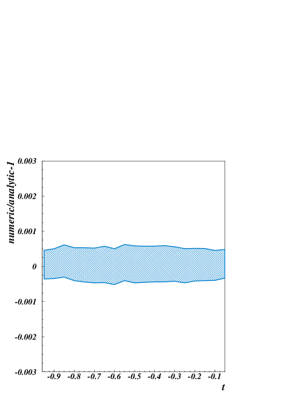
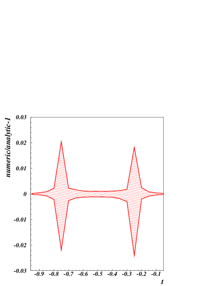
Figure 7: Results for the finite piece of the non planar box with seven propagators in the region $u,\,t<0$ and $s=-t-u$ for $s=1$ as a function of $t$. The left panels show our numerical results for the real and imaginary part (upper and lower plot respectively) and the right ones the corresponding comparisons with the analytic calculation of tausk .

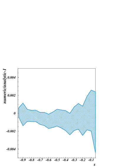
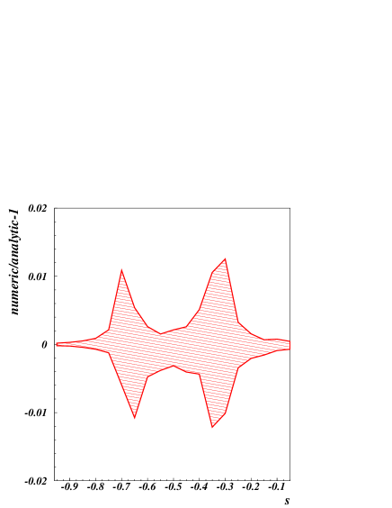
Figure 8: Results for the finite piece of the non planar box with seven propagators in the region $u,\,s<0$ and $t=-s-u$ for $t=1$ as a function of $s$. The upper and lower left panels show our numerical results for the real and imaginary parts, respectively; and the two right ones the corresponding comparisons to the analytic calculation of tausk .

In this case, the relative errors obtained by numerical integration are bigger than in the the on-shell double box. This is particularly noticeable in the imaginary part in both regions (i) and (ii), for which the relative error reaches 1-2%. However, this only happens for non-significant points of the phase-space in which the magnitude of the imaginary part is almost zero (notice that in both regions, the imaginary part of the finite term changes sign twice).

The non-planar double-box has a complicated analytic structure in terms of the kinematic invariants, since there is no Euclidean kinematic region for this integral. The two kinematic regions that we study here, require complicated analytic continuations with traditional methods. With our method, it is particularly simple to compute loop integrals in different regions of phase space. Our results demonstrate that the numerical integration of the contour integrals allows for a trivial analytic continuation in the invariants, giving correct and accurate results in all phase-space.

VI.5 Planar double-box with one leg off-shell

Our next example is the planar double-box with one external mass. The first results for this integral were obtained in sector_loop using sector decomposition. Soon afterwards it was computed analytically in smirnovB , and with differential equation method in thomas_int .

We derive a 5-fold MB representation for this integral in Section II. The integral is $1/\epsilon^{4}$ divergent; after the expansion in $\epsilon$, we find that the double and simple poles and the finite term, contain three-dimensional Mellin-Barnes integrals.

(a)

(b)

Figure 9: The two kinematical configurations considered for the double box with one massive leg. (a) the decay process $p_{4}\rightarrow p_{1}+p_{2}+p_{3}$ and (b) the scattering $p_{1}+p_{2}\rightarrow p_{3}+p_{4}$. The double line corresponds to the massive particle, $p_{4}$.

In Figure 10 we show the results for this integral in the region corresponding to the decay of a heavy particle $p_{4}\rightarrow p_{1}+p_{2}+p_{3}$ (Figure 9a), where we have fixed the mass of the particle $p_{4}^{2}=s_{123}=1$ and one of the invariants $s_{13}=(p_{1}+p_{3})^{2}=3/10$, and we consider values of $s_{23}=(p_{2}+p_{3})^{2}$ within the allowed range. Again, the relative errors are of the order of the few per mille, with highest values in the points in which the absolute value of the integral is small (in this case both the real and the imaginary components change sign).

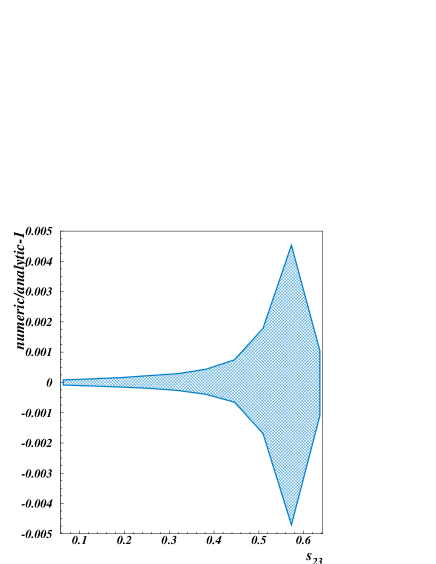
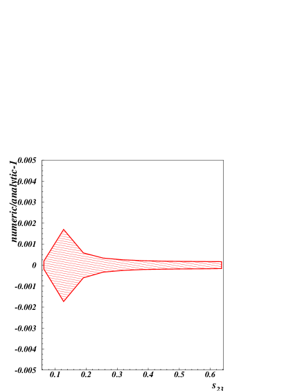
Figure 10: Results for the finite term of the double box with one leg off-shell in the physical region for the decay of a heavy particle, $p_{4}\rightarrow p_{1}+p_{2}+p_{3}$ (Figure 9a). On the upper and lower left panel we plot the real and imaginary parts as a function of the invariant $s_{23}=(p_{2}+p_{3})^{2}$ for fixed value of $p_{4}^{2}=s_{123}=1$ and $s_{13}=(p_{1}+p_{3})^{2}=3/10$. On the right panels we show the corresponding ratios of the numerical calculation to the analytic result of thomas_int for the same kinematics, the bands are given by the error in the numerical integrations.

For this topology we also considered the kinematical region corresponding to a $p_{1}+p_{2}\rightarrow p_{3}+p_{4}$ process being $p_{4}$ the massive momentum (see Fig. 9b). The corresponding results are shown in Figure 11 for fixed values of $s=(p_{1}+p_{2})^{2}=1$ and $p_{4}^{2}=1/10$ as a function of $t=(p_{2}-p_{3})^{2}$. Again we find very good agreement with the analytic results in both phase space regions.

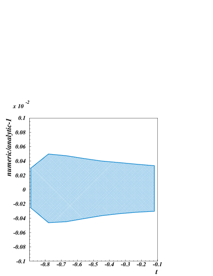
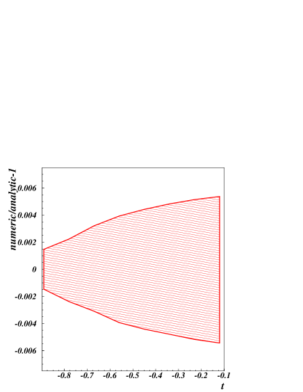
Figure 11: Results for the finite part of the double box with one leg off-shell in the physical region for a $2\rightarrow 2$ process with the massive leg on the final state (Fig. 9b). On the upper and lower left panels we plot the real and imaginary parts of $c_{0}$ as a function of the invariant $t=(p_{2}-p_{3})^{2}$ for fixed value of $s=(p_{1}+p_{2})^{2}=1$ and $p_{4}^{2}=1/10$. On the right panels we show the corresponding ratios of the numerical calculation to the analytic result of thomas_int for the same kinematics, the bands are given by the error in the numerical integrations.

VI.6 Planar double box with two adjacent massive legs

We now make one further step for the planar double box and consider the case of two external adjacent masses. This integral has been evaluated for the first time, in some points in the Euclidean region, in Binoth:2003ak .

As shown in Section II, it is possible to get a MB representation for the double box with two adjacent massive legs with six MB parameters. Again, after the analytic continuation, the effective dimensionality is reduced by factors containing gamma functions in the denominator. In the present example, only integrals in three dimensions are needed to compute the finite pieces in the series around $\epsilon=0$. Quartic and cubic poles are completely determined by the pieces with no integrals left.

We found complete agreement with the results quoted in Binoth:2003ak . We also compared our results for some values of the invariants in the Euclidean region with an independent calculation obtained with our own sector decomposition code. In Table 6 we show the results obtained by the two methods for two phase space points in the mentioned region. The invariants are defined as $s=(p_{1}+p_{2})^{2}$, $t=(p_{2}-p_{3})^{2}$, $M_{1}^{2}=p_{3}^{2}$, $M_{2}^{2}=p_{4}^{2}$ (see Figure 12 for the definition of the momenta). We find perfect agreement within the integration errors.

Point	MB	Sector Decomposition
$s=t=M_{1}^{2}=M_{2}^{2}=-1$	$$\begin{array}[]{r@{.}lcr}-0&25&&\epsilon^{-4}+\\ 0&288608&&\epsilon^{-3}+\\ -2&22227&(1)&\epsilon^{-2}+\\ -6&577&(6)&\epsilon^{-1}+\\ -10&15&(4)&\end{array}$$	$$\begin{array}[]{r@{.}lcr}-0&25&&\epsilon^{-4}+\\ 0&2886&(2)&\epsilon^{-3}+\\ -2&222&(2)&\epsilon^{-2}+\\ -6&577&(6)&\epsilon^{-1}+\\ -10&15&(2)&\end{array}$$
$$\begin{array}[]{r@{=}l}s&-1\\ t&-1/2\\ M_{1}^{2}&-7/10\\ M_{2}^{2}&-2/5\end{array}$$	$$\begin{array}[]{r@{.}lcr}-0&5&&\epsilon^{-4}+\\ 0&463887&&\epsilon^{-3}+\\ -4&47418&(1)&\epsilon^{-2}+\\ -17&46&(1)&\epsilon^{-1}+\\ -37&21&(9)&\end{array}$$	$$\begin{array}[]{r@{.}lcr}-0&5&&\epsilon^{-4}+\\ 0&4639&(5)&\epsilon^{-3}+\\ -4&474&(4)&\epsilon^{-2}+\\ -17&46&(2)&\epsilon^{-1}+\\ -37&21&(9)&\end{array}$$

Table 6: Results for the double box with two legs off-shell for two points in the Euclidean region, we show results obtained with both the Mellin-Barnes technique and wit the sector decomposition method.

Figure 12: The double box diagram with two adjacent massive legs.

We also present our results in the kinematical region corresponding to the process $p_{1}+p_{2}\rightarrow p_{3}+p_{4}$ shown in Figure 12, relevant, for instance, for the process $pp\rightarrow W^{+}W^{-}$. In Figure 13 we plot the values of the coefficients, for this configuration, up to the finite terms as a function of $t$ in the case of two equal masses, $M_{1}^{2}=M_{2}^{2}=1/10$, where the energy scale is fixed by $s=1$. Figure 14 corresponds to the same kinematical region but for $s=1$, $M_{1}^{2}=1/20$ and $M_{2}^{2}=1/2$. The error bars again lie within the points in the plot and are, for the finite pieces, typically less that 1% after a run of a couple of minutes per point on a 2.8GHZ CPU.

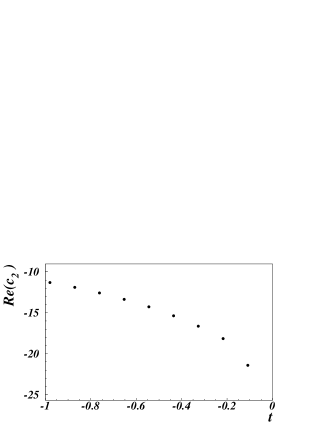
Figure 13: Results for the double box with two adjacent masses in the physical region of a $2\rightarrow 2$ process where the two particles in the final state are massive. We plot the values of the coefficients as function of $t$ for $s=1$, $M_{1}^{2}=M_{2}^{2}=1/10$.

Figure 14: Results for the double box with two adjacent masses in the physical region of a $2\rightarrow 2$ process where the two particles in the final state are massive. We plot the values of the coefficients as function of $t$ for $s=1$, $M_{1}^{2}=1/20$ and $M_{2}^{2}=1/2$.

VI.7 The on-shell massless triple box

At the three loop level, we start by considering the on-shell triple box (Figure 15), impressively computed in an analytic way in smirnovC using the MB technique.

Using the re-insertion method described in Section II, we get a 7-fold MB representation. The analytic continuation leaves us with contributions with up to 5 contour integrals for the constant pieces in the $\epsilon$ expansion, and poles up to $\epsilon^{-6}$. Although the numerical integration is certainly more involved in this case, due to the depth of the poles in $\epsilon$ which generates very complicated expressions for the finite terms, it is relatively easy to achieve a precision of $\sim 1\%$, as shown in Figure 16. As in the two loop case we show results for the physical region corresponding to $s>0$, $t<0$ with $s=(p_{1}+p_{2})^{2}$ and $t=(p_{2}-p_{3})^{2}$. We compare our results with the analytic computation of smirnovC . We used the MATHEMATICA package HPL maitre for the evaluation of the one-dimensional harmonic polylogarithms.

Figure 15: The on-shell triple box diagram.

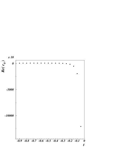
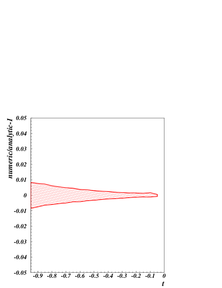
Figure 16: Results for the finite part of the planar triple box in the physical region for a $2\rightarrow 2$ process. On the upper and lower left panel we plot the real and imaginary parts, respectively, of $c_{0}$ as a function of $t$ for fixed value of $s=1$. On the right panels we show the corresponding ratios of the numerical calculation to the analytic result of smirnovC for the same kinematics, the bands are given by the error in the numerical integrations.

VI.8 The triple box with one external mass

As we did for the double box topology, we consider now a further step in complication for the triple box, adding a mass in the external state. This is, as far as we know, the first evaluation of a three-loop box with three mass scales.

We obtained a MB representation with 8 variables. As usual, the dimensionality of the problem is reduced after the analytic continuation and we found that, up to order $\epsilon^{0}$, only up to six-fold integrals contribute.

We present results for this novel integral in the physical region of the decay of a heavy particle, $p_{4}\rightarrow p_{1}+p_{2}+p_{3}$ (Figure 17) as we did in the two loops case. In Figure 18 we show the the corresponding coefficients of the expansion in $\epsilon$ as a function of the invariant $s_{23}$ for fixed values of the other two variables: $p_{4}^{2}=1$ and $s_{13}=3/10$. With the notable exception of the left-most point in the real part of the constant term, the error bars are all contained in the plotted points. They are typically of the order of $1\%$ or better for the finite parts after 50 minutes, in average, per point on a 2.8GHZ CPU.

Figure 17: The triple box in the decay process $p_{4}\rightarrow p_{1}+p_{2}+p_{3}$

Figure 18: Results for the triple box with one massive leg in the physical region of the decay of a massive particle, $p_{4}\rightarrow p_{1}+p_{2}+p_{3}$ (Figure 17). We show the results for fixed values of $p_{4}^{2}=1$ and $s_{13}=3/10$ as a function of the remaining invariant $s_{23}$.

Figure 19: Results for the triple box with one leg off-shell in the physical region for a $2\rightarrow 2$ process with the massive leg on the final state. We plot the real and imaginary parts as a function of the invariant $t=(p_{2}-p_{3})^{2}$ for fixed value of $s=(p_{1}+p_{2})^{2}=1$ and $p_{4}^{2}=1/10$.

VII Conclusions and Outlook

In this paper, we have introduced a new method for the numerical evaluation of arbitrary loop integrals. We first derive Mellin-Barnes representations by either decomposing directly the Feynman representation, or by using one-loop representations as building blocks for representations of multi-loop integrals. For a given representation, we find values of the space-time dimension and the powers of the propagators which yield a well defined representation. Then we use automated programs to perform the analytic continuation to values of the parameters for which the integral may develop divergences. Finally, we expand in $\epsilon$ and compute the integral coefficients of the expansion numerically.

The method is based on the earlier work of Smirnov smirnov and Tausk tausk . The novel features in our publication are: (i) the automation of the procedure for the $\epsilon$ expansion, (ii) the numerical evaluation of the coefficients of the expansion, avoiding cumbersome summations of multiple infinite series and the analytic continuation in the arguments of polylogarithms, (iii) and the efficient generalization of the method to tensor integrals. We believe that these new features render our method suitable for the practical evaluation of multi-loop amplitudes in gauge theories.

We have performed a number of explicit calculations to verify our algorithms and demonstrate the power of our method. We first recalculated complicated loop integrals which are only recently known in the literature. Namely, we evaluated the planar and cross on-shell double boxes, the planar double-box with one leg off-shell, and the triple planar box with on-shell legs. In all cases, we have found an excellent agreement between our numerical results and the known analytic results. The analytic results require complicated analytic continuations of polylogarithms to non-Euclidean kinematic regions. With our method, we were able to compute the integrals in all kinematic regions effortlessly.

In this paper, we have presented results for loop-integrals which were previously unknown. At two-loops, we have computed the double-box integral with two adjacent legs off-shell for independent external mass-parameters. This is one of the most complicated two-loop box integrals that enters the evaluation of two-loop amplitudes for heavy boson pair production at colliders. At three-loops, we have computed the planar triple-box with one off-shell leg; this integral emerges in $e^{+}e^{-}\to 3\mbox{ jets}$, or the production of a single heavy boson in association with a jet at hadron colliders at NNNLO in QCD. To the best of our knowledge, it is the first time that a two-loop box with four kinematic scales or a three-loop box with three scales are ever computed in all physical regions.

Many processes with six external legs are particularly important at the LHC. At present, there has been no NLO calculation of a cross-section for a hadron collider process with six external states, due to the lack of efficient methods for evaluating loop amplitudes. In this paper, we applied our method to the evaluation of tensors through rank six for the hexagon topology. The purpose of this application was two-fold; first, we wanted to demonstrate that we were able to extend the method to tensor integrals economically, and second, to setup programs that are efficient for the evaluation of multi-scale one-loop amplitudes (e.g. six parton QCD amplitudes). We have found that the evaluation of the tensor integrals is not significantly more complicated than the scalar integral. The programs that we developed can be immediately used for the evaluation of the six parton one-loop QCD amplitudes.

Our technical goals for the current study were to build the necessary programs, implement an efficient book-keeping platform, and to examine the scaling of computing intensity in applications with diverse features. We anticipate that our method can be improved and generalized even further, when we consider issues that were only briefly examined in this first study. For example, in preliminary investigations, we have found that it is possible to exploit further the Cauchy theorem. If we specify a kinematic region, it turns out that some of the numerical integrals can be approximated very accurately by the sum of a finite number of residues. We expect that we can improve substantially our efficiency if we replace some of the integrations which involve kinematic scales with appropriate finite sums of such residues. In addition, we are investigating hybrid approaches, combining our method with ideas in Ref. diff_nnlo .

The applications of our method are numerous. We believe that it will be particularly useful for precision calculations of observables in collider physics. We plan to apply our techniques to key NLO and NNLO calculations for the LHC and to answer more formal questions on the perturbative behavior of gauge theories in the near future.

References

- (1) J. Campbell, R. K. Ellis, F. Maltoni and S. Willenbrock, arXiv:hep-ph/0510362.
- (2) L. W. Garland, T. Gehrmann, E. W. N. Glover, A. Koukoutsakis and E. Remiddi, Nucl. Phys. B 642, 227 (2002) [arXiv:hep-ph/0206067].
- (3) A. Vogt, S. Moch and J. A. M. Vermaseren, Nucl. Phys. B 691, 129 (2004) [arXiv:hep-ph/0404111].
- (4) G. Passarino and M. J. G. Veltman, Nucl. Phys. B 160, 151 (1979).
- (5) F. V. Tkachov, Phys. Lett. B 100, 65 (1981); K. G. Chetyrkin and F. V. Tkachov, Nucl. Phys. B 192, 159 (1981).
- (6) T. Gehrmann and E. Remiddi, Nucl. Phys. B 580, 485 (2000) [arXiv:hep-ph/9912329].
- (7) Z. Bern, L. J. Dixon and D. A. Kosower, Nucl. Phys. B 412, 751 (1994) [arXiv:hep-ph/9306240].
- (8) A. V. Kotikov, Phys. Lett. B 254, 158 (1991).
- (9) W. T. Giele and E. W. N. Glover, JHEP 0404, 029 (2004) [arXiv:hep-ph/0402152]; R. K. Ellis, W. T. Giele and G. Zanderighi, arXiv:hep-ph/0508308; R. K. Ellis, W. T. Giele and G. Zanderighi, Phys. Rev. D 72, 054018 (2005) [arXiv:hep-ph/0506196].
- (10) A. Denner and S. Dittmaier, arXiv:hep-ph/0509141; A. Denner and S. Dittmaier, Nucl. Phys. B 658, 175 (2003) [arXiv:hep-ph/0212259];
- (11) T. Binoth, J. P. Guillet, G. Heinrich, E. Pilon and C. Schubert, arXiv:hep-ph/0504267; T. Binoth, G. Heinrich and N. Kauer, Nucl. Phys. B 654, 277 (2003) [arXiv:hep-ph/0210023];
- (12) T. Binoth, J. P. Guillet, G. Heinrich and C. Schubert, Nucl. Phys. B 615, 385 (2001) [arXiv:hep-ph/0106243]; T. Binoth, J. P. Guillet and G. Heinrich, Nucl. Phys. B 572, 361 (2000) [arXiv:hep-ph/9911342].
- (13) A. van Hameren, J. Vollinga and S. Weinzierl, Eur. Phys. J. C 41, 361 (2005) [arXiv:hep-ph/0502165].
- (14) F. del Aguila and R. Pittau, JHEP 0407, 017 (2004) [arXiv:hep-ph/0404120].
- (15) A. Denner, S. Dittmaier, M. Roth and L. H. Wieders, arXiv:hep-ph/0505042; A. Denner, S. Dittmaier, M. Roth and L. H. Wieders, Phys. Lett. B 612, 223 (2005) [arXiv:hep-ph/0502063].
- (16) Z. Nagy and D. E. Soper, JHEP 0309, 055 (2003) [arXiv:hep-ph/0308127].
- (17) Z. Bern, L. J. Dixon and D. A. Kosower, arXiv:hep-ph/0507005.
- (18) S. Laporta, Int. J. Mod. Phys. A 15, 5087 (2000) [arXiv:hep-ph/0102033].
- (19) C. Anastasiou and A. Lazopoulos, JHEP 0407, 046 (2004) [arXiv:hep-ph/0404258].
- (20) A. V. Smirnov and V. A. Smirnov, arXiv:hep-lat/0509187; O. V. Tarasov, Nucl. Instrum. Meth. A 534, 293 (2004) [arXiv:hep-ph/0403253]; O. V. Tarasov, Acta Phys. Polon. B 29, 2655 (1998) [arXiv:hep-ph/9812250]; P. A. Baikov, arXiv:hep-ph/0507053; P. A. Baikov, Nucl. Phys. Proc. Suppl. 116 (2003) 378. V. A. Smirnov and M. Steinhauser, Nucl. Phys. B 672, 199 (2003) [arXiv:hep-ph/0307088].
- (21) S. Actis, A. Ferroglia, G. Passarino, M. Passera and S. Uccirati, Nucl. Phys. B 703, 3 (2004) [arXiv:hep-ph/0402132]; A. Ferroglia, M. Passera, G. Passarino and S. Uccirati, Nucl. Phys. B 680, 199 (2004) [arXiv:hep-ph/0311186]; A. Ferroglia, M. Passera, G. Passarino and S. Uccirati, Nucl. Phys. B 650, 162 (2003) [arXiv:hep-ph/0209219]; G. Passarino and S. Uccirati, Nucl. Phys. B 629, 97 (2002) [arXiv:hep-ph/0112004]. S. P. Martin and D. G. Robertson, arXiv:hep-ph/0501132. M. Caffo, H. Czyz and E. Remiddi, Nucl. Phys. Proc. Suppl. 116, 422 (2003) [arXiv:hep-ph/0211178]; S. Laporta, Phys. Lett. B 504, 188 (2001) [arXiv:hep-ph/0102032].
- (22) T. Binoth and G. Heinrich, Nucl. Phys. B 585, 741 (2000) [arXiv:hep-ph/0004013];
- (23) T. Binoth and G. Heinrich, Nucl. Phys. B 680, 375 (2004) [arXiv:hep-ph/0305234].
- (24) K. Hepp, Commun. Math. Phys. 2, 301 (1966). M. Roth and A. Denner, “High-energy approximation of one-loop Feynman integrals,” Nucl. Phys. B 479, 495 (1996) [arXiv:hep-ph/9605420].
- (25) T. Binoth, G. Heinrich and N. Kauer, Nucl. Phys. B 654, 277 (2003) [arXiv:hep-ph/0210023].
- (26) C. Anastasiou, K. Melnikov and F. Petriello, arXiv:hep-ph/0505069.
- (27) V. A. Smirnov, Phys. Lett. B 460, 397 (1999) [arXiv:hep-ph/9905323].
- (28) J. B. Tausk, Phys. Lett. B 469, 225 (1999) [arXiv:hep-ph/9909506].
- (29) V. A. Smirnov and O. L. Veretin, Nucl. Phys. B 566, 469 (2000) [arXiv:hep-ph/9907385].
- (30) C. Anastasiou, J. B. Tausk and M. E. Tejeda-Yeomans, Nucl. Phys. Proc. Suppl. 89, 262 (2000) [arXiv:hep-ph/0005328].
- (31) V. A. Smirnov, Phys. Lett. B 491, 130 (2000) [arXiv:hep-ph/0007032]; V. A. Smirnov, Phys. Lett. B 500, 330 (2001) [arXiv:hep-ph/0011056]; V. A. Smirnov, Phys. Lett. B 524, 129 (2002) [arXiv:hep-ph/0111160]; G. Heinrich and V. A. Smirnov, Phys. Lett. B 598, 55 (2004) [arXiv:hep-ph/0406053].
- (32) V. A. Smirnov, Phys. Lett. B 567, 193 (2003) [arXiv:hep-ph/0305142].
- (33) Z. Bern, L. J. Dixon and V. A. Smirnov, Phys. Rev. D 72, 085001 (2005) [arXiv:hep-th/0505205].
- (34) C. Anastasiou, Z. Bern, L. J. Dixon and D. A. Kosower, Phys. Rev. Lett. 91, 251602 (2003) [arXiv:hep-th/0309040].
- (35) E. Remiddi and J. A. M. Vermaseren, Int. J. Mod. Phys. A 15, 725 (2000) [arXiv:hep-ph/9905237].
- (36) N.I. Ussyukina, Teor.Mat.Fiz. 22 (1975) 300; E. E. Boos and A. I. Davydychev, Theor. Math. Phys. 89, 1052 (1991) [Teor. Mat. Fiz. 89, 56 (1991)]; N. I. Ussyukina and A. I. Davydychev, Phys. Lett. B 305, 136 (1993); N. I. Ussyukina and A. I. Davydychev, Phys. Lett. B 298, 363 (1993).
- (37) T. Gehrmann and E. Remiddi, Nucl. Phys. B 601, 248 (2001) [arXiv:hep-ph/0008287].
- (38) T. Gehrmann and E. Remiddi, Comput. Phys. Commun. 141, 296 (2001) [arXiv:hep-ph/0107173].
- (39) T. Gehrmann and E. Remiddi, Comput. Phys. Commun. 144, 200 (2002) [arXiv:hep-ph/0111255].
- (40) T. Gehrmann and E. Remiddi, Nucl. Phys. B 640, 379 (2002) [arXiv:hep-ph/0207020].
- (41) Vladimir. A. Smirnov, “Evaluating Feynman Integrals”, Springer Tracts in Modern Physics 211.
- (42) T. Hahn, arXiv:hep-ph/0404043; T. Hahn, arXiv:hep-ph/0509016.
- (43) J. A. M. Vermaseren, arXiv:math-ph/0010025.
- (44) D. Maitre, arXiv:hep-ph/0507152.
- (45) C. Anastasiou, K. Melnikov and F. Petriello, Phys. Rev. D 69, 076010 (2004) [arXiv:hep-ph/0311311].