Cross sections, error bars and event distributions in simulated Drell-Yan azimuthal asymmetry measurements.

Abstract

A short summary of results of recent simulations of (un)polarized Drell-Yan experiments is presented here. Dilepton production in $pp$, $\bar{p}p$, $\pi^{-}p$ and $\pi^{+}p$ scattering is considered, for several kinematics corresponding to interesting regions for experiments at GSI, CERN-Compass and RHIC. A table of integrated cross sections, and a set of estimated error bars on measurements of azimuthal asymmetries (associated with collection of 5, 20 or 80 Kevents) are reported.

1 Introduction

The aim of this work is to give some useful reference numbers for planning Drell-Yan experiments aimed at the measurement of transverse spin/momentum related azimuthal asymmetries.

Total cross sections (nb) for several colliding particle combinations, mass ranges and S-values. M (GeV/c²) 1.5-2.5 4-9 12-40 1.5-2.5 4-9 12-40 S (GeV²) $pp$ $\bar{p}p$ 30 0.03 $<<$pb $<<$pb 1.3 0.3 pb $<<$pb 200 0.7 0.01 $<<$pb 4.4 0.35 $<<$pb (200)² 3.5-17 1.2-5.5 0.06-0.26 5-18 2.6-7 0.24-0.4 $\pi^{-}p$ $\pi^{+}p$ 30 0.9 1 pb $<<$pb 0.25 0.1 pb $<<$pb 200 1.9 0.25 $<<$pb 0.7 0.07 $<<$pb (200)² 1.8-5.6 0.75-2.1 0.1-0.2 1.5-4.8 0.5-1.4 0.04-0.1 For the high-energy case, two different parameterizations have been used, leading to pairs of $\sigma$ values. See text for details.

Figure 1: $\bar{p}p$ event scatter plot for $S$ $=$ 200 GeV², and dilepton mass in the range 4-9 GeV/c².

Figure 2: $\bar{p}p$ event scatter plot for $S$ $=$ 30 GeV², and dilepton mass in the range 1.5-2.5 GeV/c².

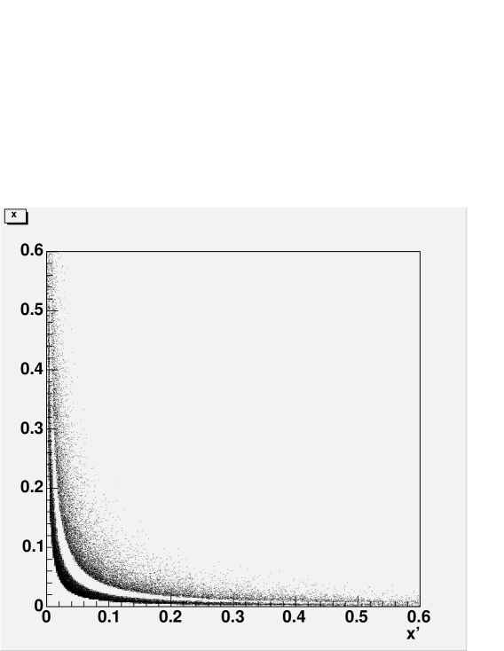
Figure 3: $pp$ event scatter plot for $S$ $=$ (200)² GeV², and dilepton mass in the double range 4-9 and 12-40 GeV/c².

Figure 4: X2-integrated distribution of the scatter plot of fig.1. Events are divided into 50 X1-bins.

This includes total cross sections for several kinematical options for $pp$, $\bar{p}p$ and $\pi_{\pm}p$ Drell-Yan dilepton production: squared hadron-CM energy $S$ $=$ 30 GeV², 200 GeV², (200)² GeV², and dilepton masses in the ranges 1.5-2.5 GeV/c², 4-9 GeV/c², 12-40 GeV/c². For some relevant situations, estimates of the asymmetry error bars are reported, for sets of 5, 20, 80 Kevents divided into 10 bins of the longitudinal fraction $x$. Previous Drell-Yan data and fitting relations[1, 2] are the basis of the initial core of the used simulation code. Several details on the formalism, together with the most recent examples of simulated asymmetries, are presented elsewhere in this workshop[3], and in published work by myself and M.Radici[4, 5].

2 Total Cross Sections.

Total cross sections are shown in table 1. For the two lower $S-$values they have been evaluated with the differential cross-section fit relations[1, 2] coming from measurements of $\pi^{-}A$ and $\bar{p}A$ at $S$ $=$ 250-400 GeV². The two cases $\pi^{-}p$ and $\bar{p}p$ correspond to these cross sections for $Z/A$ $=$ 1. For $\pi^{+}p$ we have assumed $\pi^{-}p$ $\equiv$ $\pi^{+}p$ for the pion sea contribution, $\pi^{-}p$ $\equiv$ (1/4)$\pi^{+}n$ for the pion valence contribution, and calculated $\pi^{-}A$ for $Z/A$ $=$ 0. Cross sections for $pp$ have been evaluated by substituting the $(sea+valence)(sea+valence)$ structure of $\bar{p}p$ with the structure ${1/2}[sea(sea+valence)+(sea+valence)sea]$. For the largest $S$ case the calculation based on the previous parameterization (with sea $\sim$ const for small $x$) has been sided by an alternative calculation using the (LO-intermediate gluon) MRST distributions [6], with sea $\sim$ $x^{-\lambda}$ ($\lambda$ $\approx$ 0.2-0.3 for mass $<$ 9 GeV/c), and based on data sets including several recent Drell-Yan meaasurements[7]. No evolution was applied, which is unproper for $M$ $>>$ 10 GeV/c². The $K-$factors have been assumed as constant but tuned to reproduce with both methods the measured cross sections at $S$ $=$ 250 GeV², masses 4-9 GeV/c²[2]. The former strategy leads to the smaller reported cross section values, the latter to the bigger ones. For the $\pi^{\pm}p$ high-energy case double values refer to different parameterizations for the distribution functions of the proton only, pion distribution functions have not been changed. For the lowest mass range 1.5-2.5 the smaller number of contributing quarks introduces a reduction factor $\approx$ 1/2. The difference between the other two mass ranges is not essential.

3 Event distributions

The event distribution has the general form

$$N(S,x,x^{\prime},P_{T},\xi)\ =\ F(S,x,x^{\prime},P_{T})\cdot[1\ +\ A(x,x^{\prime},P_{T},\xi)].$$ (1)

where $x,x^{\prime},P_{T}$ describe the virtual photon kinematics in the hadron center of mass ($P_{L}/(S/2)$ $\equiv$ $x-x^{\prime}$, $M^{2}/S$ $\equiv$ $xx^{\prime}$), while $\xi$ represents compactly the set of variables describing the angular distribution of the leptons in the Collins-Soper frame ($\equiv$ the photon polarization). $F(S,x,x^{\prime},P_{T})$ alone gives the virtual photon event distribution. $A(x,x^{\prime},P_{T},\xi)$ averages to zero over all the solid angle, and describes the asymmetry properties of the lepton distribution in unpolarized, single or double polarized DY.

The scatter plots of figs 1,2 and 3 reproduce the event distribution

$$N(S,x,x^{\prime})\ =\ \int d^{2}\vec{P}_{T}F(S,x,x^{\prime},P_{T})$$ (2)

for some relevant $\bar{p}p$ and $pp$ cases. Fig.4 reports

$$N(S,x)\ =\ \int dx^{\prime}N(S,x,x^{\prime})$$ (3)

where the integrated distribution is the one of fig.1. Events in the $xx^{\prime}$ scatter plots concentrate near the hyperbole $xx^{\prime}$ $=$ ${M^{2}}_{min}/S$, because $\sigma$ $\propto$ $q(x)\bar{q}(x^{\prime})/M^{2}$. For the same reason, in the case of fig.3 the lower event band ($M$ in the range 4-9 GeV/c²) contains 95 % of all the events reported in the figure.

4 Asymmetry Error Bars

Figure 5: Error bars on the azimuthal asymmetry for $\bar{p}p$, $S$ $=$ 30 GeV², dilepton mass in the range 1.5-2.5 GeV/c².

Figure 6: Error bars on the azimuthal asymmetry for $\pi^{-}p$, pion beam energy 100 GeV, fixed target, dilepton mass in the range 4-9 GeV/c².

Figure 7: Error bars on the azimuthal asymmetry for $pp$, $S$ $=$ (200)² GeV², dilepton mass in the range 12-40 GeV/c².

The integrated $N(S,x)$ distribution has its peak at $x$ $\approx$ $3{M^{2}}_{min}/S$. To the right of the peak, $N(S,x)$ $\sim$ $1/x^{n}$ with $n$ $>$ 1. This selects for each $S$, $M_{min}$ the $x-$range where error bars are smaller. The shown error bars in figs.5, 6 and 7 refer to the special case of Sivers asymmetry, however they are the same for any kind of left/right asymmetry with respect to a Collins-Soper azimuthal angle $\phi$. The asymmetry is defined as $(A-B)/(A+B)$, where $A$ and $B$ are the event numbers with positive or negative $sin(\phi-\phi_{S})$. Error bars have been calculated by assuming constant 0.05 asymmetry everywhere, and repeating the simulation 10 times to calculate fluctuations. Despite the size of the error bars is reasonably stable for $N_{repetitions}$ $>$ 5, with $N_{repetitions}$ $=$ 10 there are still small but evident fluctuations in the error bar size. This is due to most $x-$bins being filled with event numbers $N(+)+N(-)$ $<$ 1000. For $N(+)+N(-)$ $<$ 50 error bars are not shown. Typically the largest shown error bars refer to event numbers $N(+)+N(-)$ $\sim$ 100. Examination of the error bar fluctuations suggests that the reported error bars are reliable within a factor $1/\sqrt{2}\div\sqrt{2}$. If one repeats the calculation by assuming asymmetry 0 or 0.1, systematic changes of these (purely statistic) error bars are smaller than the above fluctuations. So, unless they damp asymmetries by orders, all those reducing coefficient like polarization dilution etc are not influent on the error bar sizes. For asymmetry $>$ 33 %, $N(-)$ $<$ $N(+)/2$. So, in the case of really large asymmetries, the consequent small value of $N(-)$ in those bins whose population is $<<$ 1000 introduces errors whose size may be uncontrollably larger than the estimated ones. In this case the error simulation must be more specific to be appropriate.

References

- [1] J.S.Conway et al, Phys. Rev. D39, 92 (1989).
- [2] E.Anassontzis et al, Phys. Rev. D38, 1377 (1988).
- [3] M.Radici, this workshop.
- [4] A.Bianconi and M.Radici, Phys. Rev. D34, 1729 (1980).
- [5] A.Bianconi and M.Radici Phys. Rev. D25, L527 (1992).
- [6] A.D.Martin et al, Eur. Phys. J. C4 (1998) 463, and Phys. Lett. B443 (1998) 301.
- [7] E605 collaboration, G.Moreno et al, Phys. Rev. D43 (1991) 2815, E772 collaboration, P.L.McGaughey et al, Phys. Rev. D50 (1994) 3038, NA51 collaboration, A.Baldit et al, Phys. Lett. B332 (1994) 244. E866 collaboration, E.A.Hawker et al, Phys. Rev. Lett. 80 (1998) 3715