We discuss the standard model factorizable radiative corrections to $e^{+}e^{-}\rightarrow\mu^{+}\mu^{-}\bar{b}b$, which is one of the best detection channels of the low mass Higgs boson produced through the Higgsstrahlung mechanism at a linear collider. The discussion includes the leading virtual and real quantum electrodynamics corrections due to the initial state radiation, the one-loop electroweak factorizable corrections to the on-shell Higgsstrahlung reaction and to subsequent decays of the $Z$ and Higgs boson, and the quantum chromodynamics corrections to the Higgs boson decay width into a $b\bar{b}$-quark pair.

1 Introduction

If the Higgs boson exists, it will be most probably discovered at the Large Hadron Collider. However, the precise study of its production and decay properties, which will be necessary in order to establish the Higgs mechanism as the mechanism of the electroweak (EW) symmetry breaking of the standard model (SM), can be best performed in a clean experimental environment of $e^{+}e^{-}$ collisions at a future International Linear Collider (ILC) [1].

One of the main production mechanisms of the SM Higgs boson at the ILC is the Higgsstrahlung reaction

$$e^{+}e^{-}\rightarrow ZH.$$ (1)

Reaction (1) dominates the Higgs boson production at low energies, as its cross section scales like $1/s$, at same time when cross sections of the Higgs boson production through the $WW$ and $ZZ$ boson fusion mechanisms grow with the centre of mass (CM) energy as $\ln\;(s/m^{2}_{H})$.

If the Higgs boson is light, with mass between the present $\rm{95\%\;CL}$ lower limit of $m_{H}=114.4$ GeV [2] and an upper value of, say, $m_{H}=140$ GeV, then it will decay dominantly into a pair of $b\bar{b}$ quarks. As the Z boson of reaction (1) decays into a fermion-antifermion pair too, one actually observes the Higgsstrahlung through reactions with four fermions in the final state. Precise measurements of such reactions at the ILC should be confronted with at least equally precise SM predictions, which obviously must include radiative corrections. Because of six external particles and large number of the contributing Feynman diagrams, calculation of the complete EW $\mathcal{O}(\alpha)$ corrections to reactions with four-fermion final states is very complicated. Problems encountered in the first attempt of such a complete calculation were described in [3]. Substantial progress in a full one-loop calculation for $e^{+}e^{-}\rightarrow u\bar{d}\mu^{-}\bar{\nu}_{\mu}$ was reported by the GRACE/1-LOOP team [4] and quite recently such the calculation for the charged current reactions $e^{+}e^{-}\rightarrow\nu_{\tau}\tau^{+}\mu^{-}\bar{\nu}_{\mu}$ and $e^{+}e^{-}\rightarrow u\bar{d}s\bar{c}$, which are relevant for the $W$-pair production at the ILC, has been accomplished in [5]. However, there is no calculation of the complete EW $\mathcal{O}(\alpha)$ corrections to the neutral-current $e^{+}e^{-}\rightarrow 4$ fermion processes available at the moment.

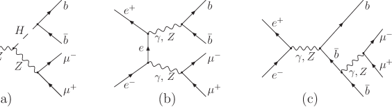
Figure 1: Examples of Feynman diagrams of reaction (2): (a) the double resonance ‘signal’, (b) and (c) ‘background’ diagrams.

Therefore, in the present lecture, we will discuss an alternative approach to the problem of improving precision of the SM predictions for the Higgs boson production and decay at the ILC through the Higgsstrahlung mechanism which has been originally proposed in [6] and recently accomplished in [7]. We will concentrate on the reaction

$$e^{+}e^{-}\rightarrow\mu^{+}\mu^{-}\bar{b}b,$$ (2)

which is one of the best detection channels of (1). Typical examples of the Feynman diagrams of reaction (2) are depicted in Fig. 1. The Higgsstrahlung ‘signal’ diagram is shown in Fig. 1a, while the diagrams in Figs. 1b and 1c represent typical ‘background’ diagrams. Altogether, in the unitary gauge and with the neglect of the Higgs boson coupling to electrons, there are 34 Feynman diagrams which contribute to (2) in the lowest order of SM. The lowest order SM cross section of reaction (2), as well as of the corresponding bremsstrahlung reaction

$$e^{+}e^{-}\rightarrow\mu^{+}\mu^{-}\bar{b}b\gamma,$$ (3)

which receives contribution from 236 Feynman diagrams, can be computed with a program ee4fg [8]. On the basis of ee4fg, we have written a dedicated program eezh4f that includes factorizable radiative corrections to (2) which will be discussed in Section 2.

2 Factorizable radiative corrections

We include the factorizable radiative corrections into the cross section of (2) according to the following master formula [7]

$$\int{\rm d}\sigma = \int{\rm d}\sigma_{\rm Born+r.m.}+\int_{E_{\gamma}<E_{\rm cut}}{\rm d}\sigma_{\rm virt+soft,univ.}^{\rm QED\;ISR}$$

$$+ \int_{E_{\gamma}>E_{\rm cut}}{\rm d}\sigma_{\rm hard}^{\rm QED\;ISR}+\int{\rm d}\sigma_{\rm virt,finite}^{\rm EW\;DPA}.$$

The first integrand on the right hand side of (2) is the effective Born cross section, calculated with the whole set of the Feynman diagrams of (2), in which we have included the bulk of quantum chromodynamics (QCD) correction to the decay of Higgs boson into a $b\bar{b}$-quark pair that can be mapped into a running $b$-quark mass. This means in practise that the constituent $b$-quark mass that is used in the calculation is replaced in the Higgs–$b\bar{b}$ Yukawa coupling with the running mass, which is about a factor 3 smaller.

The second integrand on the right hand side of (2) combines the universal infra-red (IR) singular part of the $\mathcal{O}(\alpha)$ virtual QED correction to the on-shell $Z$–Higgs production process (1) with the soft bremsstrahlung correction to (2), integrated up to the soft photon energy cut $E_{\rm cut}$. It can be written as

$${\rm d}\sigma_{\rm virt+soft,univ.}^{\rm QED\;ISR}={\rm d}\sigma_{\rm Born+r.m.}C_{\rm virt+soft,univ.}^{\rm QED\;ISR},$$ (5)

with the correction factor $C_{\rm virt+soft,univ.}^{\rm QED\;ISR}$ given by

$$C_{\rm virt+soft,univ.}^{\rm QED\;ISR}=\frac{e^{2}}{2\pi^{2}} \left[\left(\ln\frac{s}{m_{e}^{2}}-1\right)\ln\frac{2E_{\rm cut}}{\sqrt{s}}+\frac{3}{4}\ln\frac{s}{m_{e}^{2}}\right].$$ (6)

In (6), $e$ is the electric charge that is given in terms of the fine structure constant in the Thomson limit $\alpha_{0}$, $e=\left(4\pi\alpha_{0}\right)^{1/2}$. Note that the running $b$-quark mass correction is included in (5). For the sake of consistency, the same modification of the $b$-quark mass in the Higgs–$b\bar{b}$ Yukawa coupling is done also in the third term on the right hand side of (2) that represents the initial state hard bremsstrahlung contribution, i.e. the cross section of reaction (3) with the hard photon emitted from the initial state electron or positron. The integral over the hard photon phase space is performed over the full angular range of the photon momentum and from the minimum value of its energy $E_{\rm cut}$ to the very kinematical limit.

Finally, the last integrand on the right hand side of Eq. (2), ${\rm d}\sigma_{\rm virt,finite}^{\rm EW,\;DPA}$, is the IR finite part of the virtual EW $\mathcal{O}(\alpha)$ correction to reaction (2) in the double pole approximation (DPA). It can be written in the following way

$${\rm d}\sigma_{\rm virt,finite}^{\rm EW,\;DPA}=\frac{1}{2s}\left\{\left|{M^{(0)}_{DPA}}\right|^{2}{C_{\rm QED}^{\rm non-univ.}}+2{\rm Re}\left({M^{(0)^{*}}_{DPA}\delta M_{DPA}}\right)\right\}{\rm d}\Phi_{4f},$$ (7)

where $M^{(0)}_{DPA}$ and $\delta M_{DPA}$ are the lowest order matrix element and the one-loop correction, respectively, in the DPA. They are calculated with the projected four momenta $k_{i}$, $i=3,...,6$, of the final state particles, except for denominators of the $Z$ and Higgs boson propagators. The projected four momenta are obtained from the four momenta $p_{i}$, $i=3,...,6$, of reaction (2) with, to some extent arbitrary, a projection procedure which is described in [7]; ${\rm d}\Phi_{4f}$ is the four-particle Lorentz invariant phase space element and $C_{\rm QED}^{\rm non-univ.}$ denotes the IR finite non universal constant part of the $\mathcal{O}(\alpha)$ QED correction that has not been taken into account in Eq. (6). The interested reader is referred to [7] for detailed definitions of $M^{(0)}_{DPA}$, $\delta M_{DPA}$ and $C_{\rm QED}^{\rm non-univ.}$, as well as for the values of the physical input parameters used in the computation.

Numerical effects of the corrections described above are illustrated in Fig. 2, where we plot the total signal cross section of (2) in the narrow width approximation (NWA) for the $Z$ and Higgs boson. How the running $b$-quark mass correction reduces the Higgsstrahlung signal is illustrated in the upper left corner of Fig. 2, where we plot the cross section of (2) in the NWA to the lowest order (solid line)

$$\sigma_{\rm Born}^{\rm NWA}=\sigma_{e^{+}e^{-}\rightarrow ZH}^{(0)}\;\frac{\Gamma_{Z\rightarrow\mu^{+}\mu^{-}}^{(0)}}{\Gamma_{Z}^{(0)}}\;\frac{\Gamma_{H\rightarrow b\bar{b}}^{(0)}}{\Gamma_{H}^{(0)}},$$ (8)

and including the running $b$-quark mass correction (dashed line)

$$\sigma_{{\rm Born+running}\;m_{b}}^{\rm NWA}=\sigma_{e^{+}e^{-}\rightarrow ZH}^{(0)}\;\frac{\Gamma_{Z\rightarrow\mu^{+}\mu^{-}}^{(0)}}{\Gamma_{Z}^{(0)}}\;\frac{\Gamma_{H\rightarrow b\bar{b}}^{(0+{\rm r.m.})}}{\Gamma_{H}^{(0+\rm{r.m.})}},$$ (9)

as functions of the centre of mass (CM) energy. In Eqs. (8) and (9), $\sigma_{e^{+}e^{-}\rightarrow ZH}^{(0)}$ is the lowest cross section of the on-shell Higgsstrahlung reaction (1), $\Gamma_{Z\rightarrow\mu^{+}\mu^{-}}^{(0)}$ and $\Gamma_{Z}^{(0)}$ $\left(\Gamma_{H\rightarrow b\bar{b}}^{(0)}\right.$ and $\left.\Gamma_{H}^{(0)}\right)$ are the lowest order partial and total $Z$ (Higgs) boson widhts, and $\Gamma_{H\rightarrow b\bar{b}}^{(0+{\rm r.m.})}$ and $\Gamma_{H}^{(0+\rm{r.m.})}$ are the partial and total Higgs boson widhts including the running $b$ quark mass correction.

The numerical effect of the QED initial state radiation (ISR) correction is illustrated in the bottom right corner of Fig. 2, where we plot the signal lowest order and QED ISR corrected cross sections of (2) in the NWA. This correction is calculated in the structure function approach, as defined by Eq. (42) of [7]. Typical effects of the ISR, i.e. a shift in the position of the maximum and a radiative tail, are obscured by the inclusion of the running $b$ quark mass correction, which shifts the corrected cross section downwards and makes its line shape narrower, due to the reduction of the Higgs boson width. The numerical effect of the EW and the running $b$ quark mass corrections is shown in the bottom left corner of Fig. 2. Finally, the combined effect of all the factorizable corrections discussed is depicted in the upper right corner of Fig. 2. The corresponding relative corrections

$$\delta_{{\rm cor.}} = \frac{\sigma_{{\rm Born+cor.}}-\sigma_{{\rm Born}}}{\sigma_{{\rm Born}}}$$ (10)

are plotted in Fig. 3.

Table 1: Branching ratios and the lowest order Higgs boson width.

$m_{H}$	BR$\left(H\rightarrow b\bar{b}\right)$	BR$\left(H\rightarrow W^{+}W^{-}\right)$	$\Gamma^{(0)}_{H}\hskip 5.69046pt$
(GeV)	(%)	(%)	(MeV)
115	81.29	4.18	5.347
130	67.53	18.43	7.288
150	29.59	58.45	19.226
160	5.28	90.98	114.930

Figure 2: The ‘signal’ total cross section of reaction (2) including different classes of corrections $\delta_{\rm cor.}$ in the NWA as a function of the CMS energy for $m_{H}=115$ GeV.

Figure 3: The relative corrections corresponding to those of Fig. 2.

Figure 4: The total cross section of reaction (2) including all the corrections as a function of the CM energy for different values of $m_{H}$.

The total cross sections of reaction (2) including all the corrections as defined in Eq. (2) are plotted in Fig. 4 as functions of the CM energy for a few values of the Higgs boson mass. The Higgs boson production signal is clearly visible in the plots only for low values, $m_{H}=115$ GeV and $m_{H}=130$ GeV, while it becomes hardly visible for higher values of the Higgs boson mass, $m_{H}=150$ GeV and $m_{H}=160$ GeV. This effect is caused by a decrease in the branching ratio ${\rm BR}(H\rightarrow b\bar{b})$ with the growing Higgs boson mass. The values of the branching ratio ${\rm BR}(H\rightarrow b\bar{b})$, together with ${\rm BR}(H\rightarrow W^{+}W^{-})$ and the total lowest order SM Higss boson width, the latter being used in the calculation, are collected in Table 1. The Born cross section of reaction (2) without the Higgs boson exchange (solid curve) is shown in Fig. 4, too. The plots of the corrected cross sections are shifted upwards with respect to it, as they include the initial hard bremsstrahlung contribution which is integrated over the full photon phase space.

3 Summary and outlook

We have discussed the factorizable SM radiative corrections to reaction (2), which is one of the best detection channels of the light Higgs boson production through the Higgsstrahlung mechanism at the ILC. The leading virtual and real QED ISR corrections to all the lowest order Feynman diagrams of reaction (2) have been included. We have used the running $b$-quark mass in the lowest order Higgs–$b\bar{b}$ Yukawa coupling in order to include the bulk of QCD corrections to the Higgs boson decay into the $b\bar{b}$-quark pair. The complete electroweak $\mathcal{O}(\alpha)$ corrections to the on–shell $Z$–Higgs production and to the $Z$ and Higgs decay widths have been taken into account in the DPA. It has been illustrated how the corrections significantly reduce the Higgs boson production signal cross section of (2) in the NWA. Finally, we have shown how the Higgs boson production signal would be visible in the CM energy dependence of the total cross section of (2).

References

-
[1]
J.A. Aguilar-Saavedra et al. [ECFA/DESY LC Physics
Working Group Collaboration], arXiv:hep-ph/0106315;
T. Abe et al., [American Linear Collider Working Group Collaboration], arXiv:hep-ex/0106056;
K. Abe et al. [ACFA Linear Collider Working Group Collaboration], arXiv:hep-ph/0109166. - [2] R. Barate et al., Phys. Lett. B565 (2003) 61.
- [3] A. Vicini, Acta Phys. Polon. B29 (1998) 2847.
- [4] F. Boudjema et al., Nucl. Phys. Proc. Suppl. 135 (2004) 323, arXiv:hep-ph/0407079.
- [5] A. Denner, S. Dittmaier, M. Roth, L.H. Wieders, arXiv:hep-ph/0502063 and arXiv:hep-ph/0505042.
- [6] F. Jegerlehner, K. Kołodziej, T. Westwański, Nucl. Phys. Proc. Suppl. 135 (2004) 92, arXiv:hep-ph/0407071.
- [7] F. Jegerlehner, K. Kołodziej, T. Westwański, Eur. Phys. J. C 44 (2005) 195, arXiv:hep-ph/0503169.
- [8] K. Kołodziej, F. Jegerlehner, Comput. Phys. Commun. 159 (2004) 106, arXiv:hep-ph/0308114.