Equation of state from lattice QCD

Abstract

Recent results on the equation of state from lattice QCD are reviewed. The lattice technique and previous results are shortly discussed. New results for physical quark masses and two sets of lattice spacings are presented. The pressure, energy density, entropy density, speed of sound and quark number susceptibilities are determined.

1 Introduction

The equation of state (EoS) of strongly interacting matter plays an important role in understanding heavy ion collisions. It is an important input for different hydrodynamical models. In QCD with increasing temperatures ($T$) we expect a transition at some $T=T_{c}$. The dominant degrees of freedom are hadrons in the low temperature phase and colored objects in the high temperature phase. Whether there is a real first order phase transition or only a rapid cross-over is still an open question.

Since we are mostly interested in the EoS around $T_{c}$, non-perturbative methods are necessary among which lattice QCD is the most systematic one. There are at least two serious difficulties with lattice simulations. The first one is connected to the lightness of the quark masses. The cost of computations increases strongly as the quark masses decrease, therefore most lattice results were obtained with unphysically large quark masses. The second difficulty is connected to the continuum limit. Calculations are always performed at a finite lattice spacing ($a$). In order to get physical results, we have to take the $a\rightarrow 0$ limit. Since for the EoS the computational costs scale as $a^{-13}$ it is not surprising that up to very recently most results were obtained only at one set of lattice spacings.

The situation is much easier in the case of the pure gauge theory. The first problem does not exist since the quark masses are infinite. There are continuum extrapolated results both with unimproved and improved lattice actions and they show nice agreement [1, 2, 3]. There are also numerous results for the full theory with dynamical quarks which will be discussed in the following.

2 Lattice formulation

Thermodynamical quantities can be obtained from the partition function which can be given by a Euclidean path-integral:

$$Z=\int dUd\bar{\Psi}d\Psi e^{-S_{E}(U,\bar{\Psi},\Psi)},$$ (1)

where $U$ and $\bar{\Psi},\Psi$ are the gauge and fermionic fields and $S_{E}$ is the Euclidean action. The lattice regularization of this action is not unique. There are several possibilities to use improved actions which have the same continuum limit as the straightforward unimproved ones. The advantage of improved actions is that the discretization errors are reduced and therefore a reliable continuum extrapolation is possible already from larger lattice spacings. On the other hand, calculations with improved actions are usually more expensive than with the unimproved one.

Usually $S_{E}$ can be split up as $S_{E}=S_{g}+S_{f}$ where $S_{g}$ is the gauge action containing only the self interactions of the gauge fields and $S_{f}$ is the fermionic part. The gauge action has one parameter, the $g$ gauge coupling, while the parameters of $S_{f}$ are the $m_{q}$ quark masses (and in finite density studies the chemical potentials). For the fermionic action the two most widely used discretization types are the Wilson and staggered fermions.

For the actual calculations finite lattice sizes of $N_{s}^{3}N_{t}$ are used. The physical volume and the temperature are related to the lattice extensions as:

$$V=(N_{s}a)^{3}, T=\frac{1}{N_{t}a}.$$ (2)

Therefore lattices with $N_{t}\gg N_{s}$ are referred to as zero temperature lattices while the ones with $N_{t}<N_{s}$ are finite temperature lattices.

For large homogeneous systems the pressure is proportional to the free energy density. Unfortunately the free energy density ($-T/V\log Z$) cannot be measured directly. We can only measure the derivatives of $\log Z$ with respect to the parameters of the action. Then, with an integration we can obtain the pressure. This method is known as the integral method for calculating the pressure. In order to remove the divergent zero-point energy we have to subtract the pressure measured on zero temperature lattices. This subtraction makes the determination of the equation of state so difficult, since small statistical errors are needed to get reasonable uncertainties after the subtraction. Further thermodynamical quantities can be derived directly from the pressure. For example the energy density ($\epsilon$), entropy density ($s$) and speed of sound ($c_{s}$) have the following relation with the pressure:

$$\epsilon=T(\partial p/\partial T)-p, s=(\epsilon+p)T, c_{s}^{2}=\frac{dp}{d\epsilon}.$$ (3)

There is another way to obtain the energy density, which is often used in the literature. One can calculate the quantity $\epsilon-3p$ directly from the partition function.

         

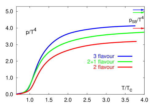
Figure 1: Left: The pressure (lower symbols) and energy density (upper symbols) with 2 flavors of unimproved staggered fermions on $N_{t}=4$ (diamonds) and $N_{t}=6$ (squares and circles) lattices for different $m_{q}/T$ ratios. [5]. Right: The pressure 2, 2+1 and 3 flavors of $p4$ improved staggered fermions on $N_{t}=4$ lattices [6].

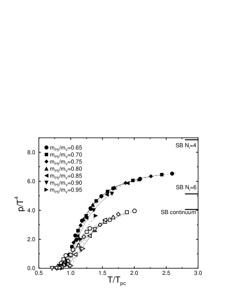
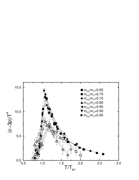
Figure 2: The pressure (left) and $\epsilon-3p$ (right) obtained from O(a) improved Wilson fermions for several pion masses on $N_{t}=4$ (filled symbols) and $N_{t}=6$ (open symbols) lattices [7]

3 Line of constant physics

Lattice calculations of the EoS are usually performed with a fixed $N_{t}$ and then, since in a fixed temperature range $N_{t}$ is inversely proportional to the lattice spacing, the continuum limit can be approached by increasing $N_{t}$. Keeping $N_{t}$ constant means that the temperature can only be varied by changing the lattice spacing. This is usually achieved by varying the $g$ gauge coupling. If we want to keep e.g. the quark masses constant then the dimensionless lattice mass parameters ($am_{q}$) have to be tuned accordingly. This defines the line of constant physics (LCP) in the parameter space.

If we keep the mass parameters constant and do not follow the LCP – which is the case in most EoS lattice studies – then we have to face the following unphysical situation. Cooling down two systems, one at $3T_{c}$ and one at $T_{c}$ to zero temperature, the quarks in the former case will be 3 times heavier. In this approach not $m_{q}$ but $m_{q}/T$ is kept constant.

The determination of the LCP is expensive since it requires hadron spectrum measurements at several lattice spacings. Furthermore, following the LCP during the determination of the EoS makes the computations more difficult, since we have to decrease the quark mass parameters with increasing temperatures. These are the reasons why most previous works ignored this physically important step of the analysis.

4 Previous results

There are numerous lattice results for the EoS using dynamical quarks. However, in all cases the quark masses – for computational reasons mentioned in the introduction – were set to higher values than their physical one. The first results were obtained with staggered fermions. Calculations were performed by the MILC collaboration [4, 5] and by Karsch, Laermann and Peikert from Bielefeld [6]. The first calculation with Wilson fermions was done by the CP-PACS collaboration [7].

Staggered results are shown on Fig. 1. No LCP was used in these cases, which means that the curves correspond to constant $m_{q}/T$, i.e. increasing quark masses with increasing temperature. Fig. 2 shows the EoS obtained with Wilson fermions for $N_{t}=4$ and 6. The lowest quark mass used here corresponds to a pion mass of $\approx 500$ MeV. The LCP was used in this analysis.

In the last years small nonzero chemical potentials [8, 9] have also been used to determine the EoS [10, 11, 12, 13].

Recently, at the lattice conference both the MILC collaboration [14] and the RBC-Bielefeld collaboration [15] reported on their ongoing work in QCD thermodynamics.

Although the published results all apply QCD with dynamical quarks they still have several weaknesses.

1. In all cases, unphysical quark masses were used, which results in unphysical pion masses. Since the transition temperature is higher than the physical mass of the pion, but smaller than the pion masses used in these calculations, it might be important to use physical values.

2. The works with staggered fermions did not use the line of constant physics which results in an unphysical dependence of the hadron masses on the temperature.

3. A known problem with staggered fermions is the taste symmetry violation which causes a non-physical non-degeneracy of the pion masses. This non-degeneracy dissapears in the continuum limit, but it is still large for the lattics spacings used in these calculations.

4. The approximate R algorithm [16] was used for the calculations with 2,3 or 2+1 flavors of staggered fermions. This algorithm has an intrinsic stepsize which leads to systematic errors in the results. In order to eliminate this systematics an extrapolation to zero stepsize should be performed. None of the previous works have done such an extrapolation. It should be mentioned that due to the subtraction in the calculation of the pressure the error coming from the typically used finite stepsizes is comparable with the result itself.

5. The discretization errors are still probably large. This is especially true for temperatures around and below $T_{c}$ where the lattice spacing of $N_{t}=4$ lattices can be as large as 0.3 fm.

6. The determination of the physical scale is not always unambiguous. Ref. [6] uses e.g. the string tension which is – strictly speaking – not an existing quantity in full QCD since at large distances the string breaks and a meson pair is produced.

5 New results with physical quark masses

In the following the new results obtained in collaboration with Y. Aoki, Z. Fodor and K.K. Szabó are presented. Details of this work are found in Ref. [17]. We have determined the EoS for two sets of lattice spacings, $N_{t}=4$ and $6$. We improved on all points listed above.

5.1 Lattice action, LCP

The lattice action we used was a combination of the tree level Symanzik-improved gauge action and the stout-improved fermionic action [18]. The stout improvement is known to reduce the taste symmetry violation significantly. This is illustrated on Fig. 3 where the pion mass splittings of the stout-improved action, the Bielefeld p4 action and the unimproved staggered action (used by previous MILC calculations) are compared.

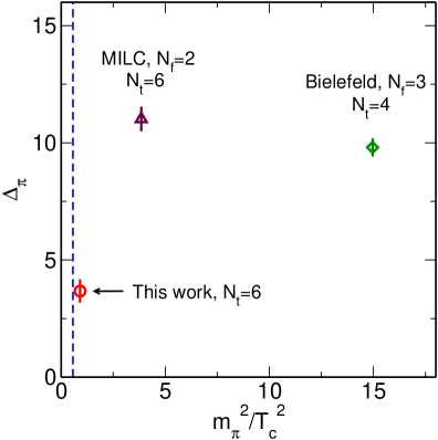
Figure 3: Pion mass splitting $\Delta_{\pi}=(m_{\pi}^{\prime 2}-m_{\pi}^{2})/T_{c}^{2}$ as a function of $(m_{\pi}/T_{c})^{2}$. The lattice spacings are the same as those at the finite temperature transition point. The mass of the Goldstone pion is denoted by $m_{\pi}$, that of the first non-Goldstone mode is by $m_{\pi}^{\prime}$. The horizontal blue line corresponds to the physical value of $(m_{\pi}/T_{c})^{2}$, where $T_{c}=173$MeV was assumed [21].

As mentioned above, using an approximate algorithm without performing the necessary extrapolations is dangerous. Instead we used the exact rational hybrid Monte-Carlo (RHMC) algorithm [19, 20].

The quark masses were set to their physical values so that the meson masses agree with their physical values up to a few percent. Moreover, the physical quark masses were kept constant while increasing the temperature, i.e. we followed the LCP. In order to determine the LCP we performed three flavor $T=0$ simulations. According to leading order chiral perturbation theory, if we set the masses of all three flavors to the mass of the strange quark, we have

$$m_{PS}^{2}/m_{V}^{2}|_{m_{q}=m_{s}}=(2m_{K}^{2}-m_{\pi}^{2})/m_{\phi}^{2},$$ (4)

This equation was used to set the strange quark mass for different lattice spacings (different temperatures at finite $T$). For the light quarks we used $m_{ud}=m_{s}/25$. This approximate determination of the LCP turned out to be sufficient. The uncertainties coming from the LCP were negligible.

As discussed previously, the determination of the EoS requires both $T>0$ and $T=0$ simulations. In the finite temperature case the derivatives of the partition function were determined for several gauge couplings (we had 16 points for $N_{t}=4$ and 14 points for $N_{t}=6$) and then the integral method was applied to get the pressure. At $T=0$ chiral perturbation theory can be used to give the quark mass dependence of the chiral condensates needed for the integration. Therefore we used four pion masses – somewhat larger then the physical one – and performed the integration for the pressure with the help of chiral perturbation theory. The four pion masses corresponded to 3,5,7 and 9 times the physical quark masses.

In order to give the EoS in $T/T_{c}$ units, we had to find the ratio of the scales at the different simulation points. For this we matched the static quark-antiquark potential for the different points at an intermediate distance. $T_{c}$ was defined as the turning point of the isospin number susceptibility ($\chi_{I}$, see later). The precise determination of $T_{c}$, i.e. connecting the scale to physical quantities will be the subject of a subsequent publication.

5.2 Results

In order to present the $N_{t}=4$ and $6$ results on the same plots we rescale all quantities in the following way. At infinite temperatures all quantities should approach their free Stefan-Boltzmann limit ($c$). This limit is, however different in the continuum ($c_{cont}$) and on lattices with some fixed $N_{t}$ ($c_{N_{t}}$). Therefore all results are scaled with a factor $c_{cont}/c_{N_{t}}$ so that they could be compared with the continuum Stefan-Boltzmann limits.

Fig. 4 shows the pressure and the energy density normalized by $T^{4}$. For comparison, the Stefan-Boltzmann limit is also shown. We can see the entropy density and the speed of sound on Fig. 5. All quantities were directly obtained from the pressure as described previously (3).

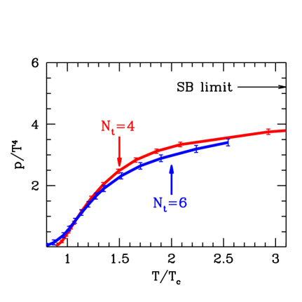
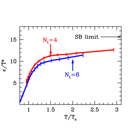
Figure 4: Left: the pressure $p$, as a function of the temperature. Both $N_{t}$=4 (red, upper curve) and $N_{t}$=6 (blue, lower curve) data are obtained along the LCP. They are normalized by $T^{4}$ and scaled by $c_{cont}/c_{N_{t}}$. In order to lead the eye lines connect the data points. Right: the energy density ($\epsilon$), red (upper) and blue (lower) for $N_{t}$=4 and 6 respectively. This result was obtained directly from the pressure.

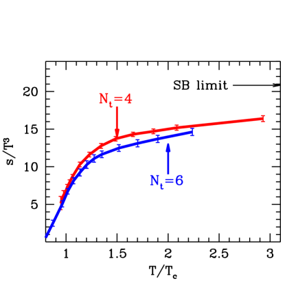
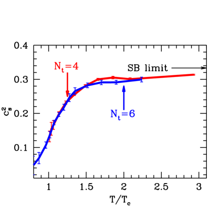
Figure 5: Left: the entropy density, normalized by $T^{3}$. Right: the speed of sound squared. The labeling is the same as for Figure 4.

The light and strange quark number susceptibilities ($\chi_{ud}$ and $\chi_{s}$) are defined as

$$\frac{\chi_{q}}{T^{2}}=\frac{1}{TV}\left.\frac{\partial^{2}\log Z}{\partial\mu_{q}^{2}}\right|_{\mu_{q}=0},$$ (5)

where $\mu_{ud}$ and $\mu_{s}$ are the light and strange quark chemical potentials. With the help of the quark number operators one can split up the quark number susceptibilities into connected and disconnected parts (see [17] for details). The disconnected parts turned out to be consistent with zero and negligible compared to the connected parts. The connected part of $\chi_{ud}$ is twice the isospin number susceptibility $\chi_{I}$.

Fig. 6 shows our results on $\chi_{I}$ and the connected part of $\chi_{s}$. Again the data are scaled by $c_{cont}/c_{N_{t}}$. The turning point of $\chi_{I}$ was used to define $T_{c}$.

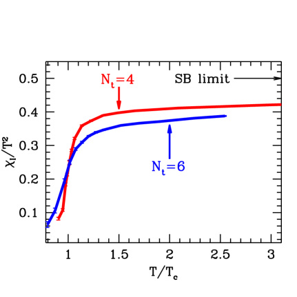
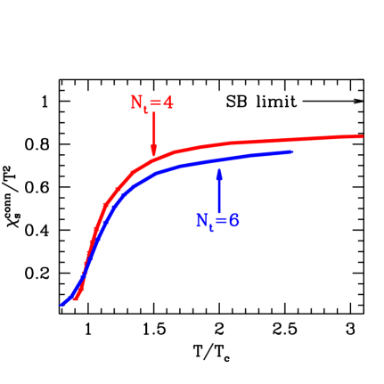
Figure 6: Left: the isospin susceptibility normalized by $T^{2}$. Right: the connected part of the strangeness susceptibility. The labeling is the same as in Figure 4.

6 Summary

The EoS can be determined using lattice QCD. While for the pure gauge theory there are already continuum extrapolated results, in full QCD there are no final results yet.

Previous results using either staggered of Wilson fermions were discussed. They suffer from several weaknesses.

In the second part of the paper new results on the EoS were presented. Our analysis attempted to improve on previous analyses by several means. We used for the lightest hadronic degree of freedom the physical pion mass. We used two different sets of lattice spacings ($N_{t}$=4,6). The system was kept on the line of constant physics (LCP) instead of changing the physics with the temperature. Due to our smaller lattice spacing and particularly due to our stout-link improved fermionic action the unphysical pion mass splitting was much smaller than in any previous staggered analysis. An exact calculation algorithm was applied.

We presented results for the pressure, energy density, entropy density, speed of sound and the isospin and strangeness susceptibilities.

Although a continuum extrapolation could already be performed with the current data, since the $N_{t}=4$ lattices are rather coarse (especially around and below $T_{c}$) it would be safer if the EoS on even finer lattices ($N_{t}$=8) were obtained. Such an analysis would be a major step towards the final results for the equation of state.

7 Acknowledgments

I thank Y. Aoki, Z. Fodor and K.K. Szabó for the nice collaboration and useful comments on the manuscript. This work was partially supported by OTKA Hungarian Science Grants No. T34980, T37615, M37071, T032501. This research is part of the EU Integrated Infrastructure Initiative Hadron physics project under contract number RII3-CT-20040506078. The computations were carried out at Eötvös University on the 330 processor PC cluster of the Institute for Theoretical Physics and the 1024 processor PC cluster of Wuppertal University.

References

- [1] G. Boyd, J. Engels, F. Karsch, E. Laermann, C. Legeland, M. Lutgemeier and B. Petersson, Nucl. Phys. B 469 (1996) 419 [arXiv:hep-lat/9602007].
- [2] M. Okamoto et al. [CP-PACS Collaboration], Phys. Rev. D 60 (1999) 094510 [arXiv:hep-lat/9905005].
- [3] Y. Namekawa et al. [CP-PACS Collaboration], Phys. Rev. D 64 (2001) 074507 [arXiv:hep-lat/0105012].
- [4] T. Blum, L. Karkkainen, D. Toussaint and S. A. Gottlieb, Phys. Rev. D 51 (1995) 5153 [arXiv:hep-lat/9410014].
- [5] C. W. Bernard et al. [MILC Collaboration], Phys. Rev. D 55 (1997) 6861 [arXiv:hep-lat/9612025].
- [6] F. Karsch, E. Laermann and A. Peikert, Phys. Lett. B 478 (2000) 447 [arXiv:hep-lat/0002003].
- [7] A. Ali Khan et al. [CP-PACS collaboration], Phys. Rev. D 64 (2001) 074510 [arXiv:hep-lat/0103028].
- [8] Z. Fodor and S. D. Katz, Phys. Lett. B 534 (2002) 87 [arXiv:hep-lat/0104001].
- [9] Z. Fodor and S. D. Katz, JHEP 0203 (2002) 014 [arXiv:hep-lat/0106002].
- [10] Z. Fodor, S. D. Katz and K. K. Szabo, Phys. Lett. B 568 (2003) 73 [arXiv:hep-lat/0208078].
- [11] R. V. Gavai and S. Gupta, Phys. Rev. D 68 (2003) 034506 [arXiv:hep-lat/0303013].
- [12] C. R. Allton, S. Ejiri, S. J. Hands, O. Kaczmarek, F. Karsch, E. Laermann and C. Schmidt, Phys. Rev. D 68 (2003) 014507 [arXiv:hep-lat/0305007].
- [13] F. Csikor, G. I. Egri, Z. Fodor, S. D. Katz, K. K. Szabo and A. I. Toth, JHEP 0405 (2004) 046 [arXiv:hep-lat/0401016].
- [14] C. Bernard et al., arXiv:hep-lat/0509053.
- [15] C. Jung, arXiv:hep-lat/0510035.
- [16] S. A. Gottlieb, W. Liu, D. Toussaint, R. L. Renken and R. L. Sugar, Phys. Rev. D 35 (1987) 2531.
- [17] Y. Aoki, Z. Fodor, S.D. Katz, K.K. Szabo, hep-lat/0510084
- [18] C. Morningstar and M. J. Peardon, Phys. Rev. D 69 (2004) 054501 [arXiv:hep-lat/0311018].
- [19] M. A. Clark, B. Joo and A. D. Kennedy, Nucl. Phys. Proc. Suppl. 119 (2003) 1015 [arXiv:hep-lat/0209035].
- [20] M. A. Clark and A. D. Kennedy, Nucl. Phys. Proc. Suppl. 129 (2004) 850 [arXiv:hep-lat/0309084].
- [21] F. Karsch, E. Laermann and A. Peikert, Nucl. Phys. B 605 (2001) 579 [arXiv:hep-lat/0012023].