High-precision determination of the light-quark masses from realistic lattice QCD

Abstract

Three-flavor lattice QCD simulations and two-loop perturbation theory are used to make the most precise determination to date of the strange-, up-, and down-quark masses, $m_{s}$, $m_{u}$, and $m_{d}$, respectively. Perturbative matching is required in order to connect the lattice-regularized bare-quark masses to the masses as defined in the $\overline{\text{MS}}$ scheme, and this is done here for the first time at next-to-next-to leading (or two-loop) order. The bare-quark masses required as input come from simulations by the MILC collaboration of a highly-efficient formalism (using so-called “staggered” quarks), with three flavors of light quarks in the Dirac sea; these simulations were previously analyzed in a joint study by the HPQCD and MILC collaborations, using degenerate $u$ and $d$ quarks, with masses as low as $m_{s}/8$, and two values of the lattice spacing, with chiral extrapolation/interpolation to the physical masses. With the new perturbation theory presented here, the resulting $\overline{\text{MS}}$ masses are $m^{\text{$\overline{\text{MS}}$}}_{s}(2~{}\mbox{GeV})=87(0)(4)(4)(0)$ MeV, and $\hat{m}^{\text{$\overline{\text{MS}}$}}(2~{}\mbox{GeV})=3.2(0)(2)(2)(0)$ MeV, where $\hat{m}={\textstyle{\frac{1}{2}}}(m_{u}+m_{d})$ is the average of the $u$ and $d$ masses. The respective uncertainties are from statistics, simulation systematics, perturbation theory, and electromagnetic/isospin effects. The perturbative errors are about a factor of two smaller than in an earlier study using only one-loop perturbation theory. Using a recent determination of the ratio $m_{u}/m_{d}=0.43(0)(1)(0)(8)$ due to the MILC collaboration, these results also imply $m^{\text{$\overline{\text{MS}}$}}_{u}(2~{}\mbox{GeV})=1.9(0)(1)(1)(2)$ MeV and $m^{\text{$\overline{\text{MS}}$}}_{d}(2~{}\mbox{GeV})=4.4(0)(2)(2)(2)$ MeV. A technique for estimating the next order in the perturbative expansion is also presented, which uses input from simulations at more than one lattice spacing; this method is used here in the estimate of the systematic uncertainties.

I Introduction

The strong sector of the standard model contains a number of inputs that are a priori unknown and must be determined from experiment. Knowledge of these fundamental parameters, the quark masses and the strong coupling, also requires precise theoretical input, because of confinement: quarks and gluons cannot be observed as isolated particles, hence one can only extract their properties by solving QCD for observable quantities such as hadron masses, as functions of the quark masses and the strong coupling. Precise values of the quark masses in particular are valuable in many phenomenological applications, such as in placing constraints on new physics beyond the standard model.

Recent breakthroughs in lattice QCD are having a significant impact on the determination of many hadronic quantities. These advances are due to two related developments: the use of perturbation theory in the design of so-called improved-lattice discretizations Viability ; ImprovedStaggered , which significantly reduces cutoff effects; and numerical simulations of a highly-efficient formalism (using so-called “staggered” quarks), where the correct number of light-quark flavors can be included in the Dirac sea, and at sufficiently small quark masses MILCsims , enabling accurate chiral extrapolations to the physical region StaggeredChiral ; MILCchiral . These developments have eliminated the large and frequently uncontrolled systematic uncertainties inherent in most other lattice QCD studies, where the effects of sea quarks are either completely neglected (working in the so-called “quenched” approximation), or where the simulations are done with the wrong number of sea quarks (and at very heavy masses): comparison of the predictions of such unrealistic theories with experiment reveals typical inconsistencies of 10–20%, which precludes their use in many important phenomenological applications.

Recent work by our group, the High Precision QCD (HPQCD) collaboration, together with the Fermilab and MILC collaborations, has instead utilized unquenched simulations with up, down and strange quarks in the Dirac sea. These simulations are made computationally feasible by using the $O(a^{2})$-improved staggered-quark action ($a$ is the lattice spacing), with the one-loop $O(a^{2})$-improved gluon action (hereafter collectively referred to as the “asqtad” action ImprovedStaggered ; MILCsims ). We have shown that these three-flavor simulations give results for a wide variety of observables that agree with experiment to within systematic errors of 3% or less Confronts . This precision, and the unified description of hadronic physics in many different systems, is a striking consequence of having a realistic description of the Dirac sea.

The application of this program to many other quantities of interest requires additional use of perturbation theory, in order to properly match lattice discretizations of the relevant operators and couplings onto continuum QCD. These perturbative-matching calculations must generally be carried out at next-to-next-to-leading order (“NNLO” order, which is generally equivalent to two-loop Feynman diagrams), if one is to obtain results of a few-percent precision HReview ; QThesis . The success of this approach has been demonstrated by a recent HPQCD determination of the strong coupling at NNLO order, with the result $\alpha_{\text{$\overline{\text{MS}}$}}(M_{z})=0.1170(12)$ HPQCDalphas , the most accurate of any method.

In this paper we apply our perturbation theory program to make the first-ever NNLO determination of the light-quark masses (the computationally-simpler case of the additive zero-point renormalization for Wilson fermions was previously computed at two-loop order in Ref. Panagop , and for static quarks in Ref. HellerMartinelli ). The quark masses are not physically measurable, and as such are only well defined in certain renormalization schemes, such as the $\overline{\text{MS}}$ mass $m^{\text{$\overline{\text{MS}}$}}(\mu)$, evaluated at some relevant scale $\mu$. We have done the necessary perturbative matching calculations to connect the lattice-regularized bare mass $m_{0}(a)$ for the “asqtad” action, as a function of the lattice spacing, to $m^{\text{$\overline{\text{MS}}$}}(\mu)$.

The lattice spacings and bare quark masses are required as input, and these have been determined in earlier studies. The lattice spacings we use were determined ultimately from the $\Upsilon^{\prime}-\Upsilon$ mass difference Upsilon , which is insensitive to the quark masses; the results agree within systematic errors of 1.5–3% with the lattice spacing extracted from a wide variety of other physical quantities Confronts ; HPQCDalphas ; this eliminates an uncontrolled systematic error in studies that are done without the correct number of sea quarks.

The bare quark masses have previously been determined in a joint HPQCD and MILC collaboration study OneLoopMass , using partially-quenched chiral-perturbation theory StaggeredChiral ; MILCchiral to make precise extrapolations to the physical region; the simulations used equal dynamical $u/d$ quark masses as small as $m_{s}/8$. These bare masses were used in Ref. OneLoopMass to estimate the $\overline{\text{MS}}$ masses using one-loop perturbation theory Hein ; the dominant systematic error in that determination came from unknown second and higher orders in the perturbative matching. Significant progress is made here due to our computation of the second-order perturbative matching coefficient. We thereby reduce the systematic error from perturbation theory by about a factor of two compared to the earlier result of Ref. OneLoopMass . The remaining perturbative error is the same size as the current lattice systematic error, which is largely due to the chiral extrapolation/interpolation.

The staggered-quark formalism had previously been afflicted with several poorly-understood problems, which have been tamed with an aggressive program of perturbative improvement, leading to the “asqtad” action that we are using here. With an unimproved-staggered action large discretization errors appear, although they are formally only $\mathcal{O}(a^{2})$ or higher. Many of the renormalization factors required to match lattice operators onto continuum quantities are also large and poorly convergent in perturbation theory for unimproved-staggered quarks; this is true, for example, of the mass renormalization that is needed here. It turns out that both problems have the same source, a particular form of discretization error dubbed “taste violation,” and both are ameliorated by use of the improved-staggered formalism ImprovedStaggered . The perturbation theory then shows small renormalizations HReview ; QThesis ; Hein ; LeeSharpePT ; HQalphaPT , and discretization errors are much reduced MILCsims . Taste violation is strongly probed in certain quantities, notably the would-be Goldstone meson masses which play an important role in our analysis, and these effects are taken into account in the staggered chiral-perturbation theory StaggeredChiral .

A potentially more fundamental concern about staggered fermions relates to the need to take the fourth root of the quark determinant, in order to convert the four-fold duplication of “tastes” into one quark flavor. One might imagine that the fourth root would introduce nonlocalities (and would induce violations of unitarity), which would prevent decoupling of the ultraviolet modes of the theory in the continuum limit. However a great deal of theoretical evidence has been amassed which demonstrates that the properties of the staggered theory, with the fourth root, are equivalent to a one-flavor theory, up to the expected discretization errors Confronts ; these are again due to short-distance taste-changing interactions, which are mediated by high-momentum gluons ImprovedStaggered . The locality of the free-field staggered theory is trivial, and is made manifest in the “naive” basis used in Ref. ImprovedStaggered . Non-localities do not arise in perturbation theory, since the staggered-quark matrix is diagonal in the taste basis, up to those short-distance (and calculable) corrections. Most important, it has been shown that perturbative improvement of staggered actions correlates exceedingly well with nonperturbatively-measured properties of the staggered-fermion matrix, providing clear support for the correctness of the fourth-root procedure. This includes the measured pattern of low-lying eigenvalues of the staggered matrix Eigenvalues , and the measured pattern of taste-violating mass differences in the non-chiral pions TasteChanging .

The rest of this paper is organized as follows. Section II details the computation of the two-loop matching factor, using the pole mass as an intermediate matching quantity. In Sect. III we use the bare-quark masses from the MILC “asqtad” simulations to extract the $\overline{\text{MS}}$ masses, including an analysis of the systematic uncertainties. In that connection, we also describe how our perturbation theory results can be used to estimate the third order in the perturbative expansion, using input from simulations at more than one lattice spacing. Section IV presents some conclusions, including a comparison of our results with other recent determinations of the strange-quark mass.

II Perturbation Theory

II.1 Lattice to $\overline{\text{MS}}$ matching

We do two-loop perturbative matching to connect the cutoff-dependent lattice bare-quark masses $m_{0}(a)$ to the $\overline{\text{MS}}$ masses $m^{\text{$\overline{\text{MS}}$}}(\mu)$ at a given scale $\mu$. We define the perturbative matching factor $Z_{m}(\mu a,m_{0}a)$ according to

$$m^{\text{$\overline{\text{MS}}$}}(\mu)=\frac{(a\,m_{0})}{a}\;Z_{m}(\mu a,m_{0}a),$$ (1)

where we make explicit the fact that the simulation input provides the bare masses in lattice units. We compute $Z_{m}$ in two stages, using the pole mass $M$ as an intermediate matching quantity. We also use our previous determination HQalphaPT ; HPQCDalphas of the relation between the lattice bare coupling $\alpha_{\rm lat}$ and the renormalized coupling $\alpha_{V}(q)$, defined by the static potential, to reorganize both sides of the matching equation into series in terms of $\alpha_{V}(q^{*})$, at an appropriately-determined scale.

In the following subsections we consider in turn the pole mass in the $\overline{\text{MS}}$- and lattice-regularization schemes. We also provide some details on the consistent evaluation of the two-loop on-shell condition in the lattice scheme, and the various checks that we have applied to our evaluation of the two-loop self-energy. We then quote our results for the matching factor of Eq. (1), and for the relevant matching scale $q^{*}$.

II.2 Pole mass in the $\overline{\text{MS}}$ scheme

We begin by recalling the relation between the $\overline{\text{MS}}$ mass and the pole mass $M$ Tarrach ; Broadhurst , which is known through three loops Chetyrkin ; Melnikov . We require it to second order, a result that was first obtained in Ref. Broadhurst (expressions for the relation at arbitrary $\mu$ are conveniently given in Ref. Chetyrkin )

$$m^{\text{$\overline{\text{MS}}$}}(\mu)=M\Biggl{[}1+z_{1}\left(\frac{\mu}{M}\right)\frac{\alpha_{\text{$\overline{\text{MS}}$}}(\mu)}{\pi}$$

$$+z_{2}\left(\frac{\mu}{M}\right)\frac{\alpha^{2}_{\text{$\overline{\text{MS}}$}}(\mu)}{\pi^{2}}+\ldots\Biggr{]},$$ (2)

where the one- and two-loop coefficient functions $z_{1}(\mu/M)$ and $z_{2}(\mu/M)$ are reduced to a set of terms with different color structures [in the following $C_{F}=(N_{c}^{2}-1)/(2N_{c})$, $C_{A}=N_{c}$, and $T=1/2$]

$$z_{1}=C_{F}z_{F},$$

$$z_{2}=C_{F}^{2}z_{FF}+C_{F}C_{A}z_{FA}+C_{F}Tn_{\ell}z_{FL}+C_{F}Tz_{FH},$$ (3)

and where the contribution $z_{FH}$ from an internal-quark loop with the same flavor as the valence quark is split off from the contribution $z_{FL}$ of $n_{\ell}$ internal-quark loops with different flavor (these are taken here to be degenerate in mass, though this is trivially generalized). The total number of flavors is $n_{f}=n_{\ell}+1$. The individual functions are given by

$$z_{F}=-1-{\textstyle{\frac{3}{4}}}\ell_{\mu M},$$

$$z_{FF}={\textstyle{\frac{7}{128}}}-{\textstyle{\frac{15}{8}}}\zeta_{2}-{\textstyle{\frac{3}{4}}}\zeta_{3}+3\zeta_{2}\log 2+{\textstyle{\frac{21}{32}}}\ell_{\mu M}+{\textstyle{\frac{9}{32}}}\ell_{\mu M}^{\,2},$$

$$z_{FA}=-{\textstyle{\frac{1111}{384}}}+{\textstyle{\frac{1}{2}}}\zeta_{2}+{\textstyle{\frac{3}{8}}}\zeta_{3}-{\textstyle{\frac{3}{2}}}\zeta_{2}\log 2-{\textstyle{\frac{185}{96}}}\ell_{\mu M}-{\textstyle{\frac{11}{32}}}\ell_{\mu M}^{\,2},$$

$$z_{FL}={\textstyle{\frac{71}{96}}}+{\textstyle{\frac{1}{2}}}\zeta_{2}-2\Delta(r_{\rm sea})+{\textstyle{\frac{13}{24}}}\ell_{\mu M}+{\textstyle{\frac{1}{8}}}\ell_{\mu M}^{\,2},$$

$$z_{FH}={\textstyle{\frac{71}{96}}}+{\textstyle{\frac{1}{2}}}\zeta_{2}-2\Delta(1)+{\textstyle{\frac{13}{24}}}\ell_{\mu M}+{\textstyle{\frac{1}{8}}}\ell_{\mu M}^{\,2},$$ (4)

where $\ell_{\mu M}\equiv\log(\mu^{2}/M^{2})$,

$$r_{\rm sea}\equiv\frac{m_{\rm sea}}{m_{\rm valence}},$$ (5)

and where $m_{\rm sea}$ and $m_{\rm valence}$ are the sea- and valence-quark masses, respectively. The function $\Delta(r)$ gives the dependence of the renormalization factors $z_{FL}$ and $z_{FH}$ on the quark mass in an internal-quark loop (sea and valence, respectively). An exact integral expression for $\Delta(r)$ can be found in Broadhurst ; particular limits are

$$\Delta(r\ll 1)={\textstyle{\frac{3}{4}}}\zeta_{2}\,r+O(r^{2}),$$

$$\Delta(1)=\frac{\pi^{2}-3}{8},$$

$$\Delta(r\gg 1)={\textstyle{\frac{1}{4}}}\log^{2}r+{\textstyle{\frac{13}{24}}}\log r$$

$$\ \ \ \ +{\textstyle{\frac{1}{4}}}\zeta_{2}+{\textstyle{\frac{151}{288}}}+O(r^{-2}\log r).$$ (6)

II.3 Pole mass in the lattice scheme

The relation between the pole mass $M$ and the bare quark mass $m_{0}(a)$ in the lattice-regularized theory has the form

$$M =m_{0}\Bigl{[}1+\alpha_{\rm lat}\left(A_{11}\log m_{0}a+A_{10}\right)$$

$$+\alpha_{\rm lat}^{2}\left(A_{22}\log^{2}m_{0}a+A_{21}\log m_{0}a+A_{20}\right)+\ldots\Bigr{]},$$ (7)

where $\alpha_{\rm lat}(a)$ is the bare lattice-regularized coupling. The coefficients of the logarithms are determined by the anomalous dimension in $m_{0}(a)$, which in turn can be determined from the known anomalous dimension of the $\overline{\text{MS}}$ mass, as described in Ref. QLattice . This also requires the connection between $\alpha_{\rm lat}$ and $\alpha_{\text{$\overline{\text{MS}}$}}$, which can be found from our evaluation of the relation between $\alpha_{\rm lat}$ and $\alpha_{V}(q)$, which we obtained at NNLO order in Refs. HQalphaPT ; HPQCDalphas (see also Ref. Schroder ); here we only require the NLO relation

$$\alpha_{\rm lat}=\alpha_{V}(q)\left[1-v_{1}(q)\alpha_{V}(q)+\ldots\right],$$ (8)

where

$$v_{1}(q)=\frac{\beta_{0}}{4\pi}\ln\left(\frac{\pi}{aq}\right)^{2}+v_{10},\quad\beta_{0}=11-\frac{2}{3}n_{f},$$ (9)

and where the constant $v_{10}$ for the “asqtad” action is

$$v_{10}=3.57123(17)-1.196(53)\times 10^{-4}\,n_{f}.$$ (10)

We then obtain (SU(3) color is used throughout) QLattice

$$A_{11}=2/\pi,$$

$$A_{22}=0.7599-0.03377\,n_{f},$$

$$A_{21}=-4.2164+0.09429\,n_{f}-0.6366\,A_{10}.$$ (11)

The terms $A_{10}$ and $A_{20}$ require the computation of the one- and two-loop lattice self-energies, respectively. We have previously determined the first-order term for the “asqtad” action Hein ; OneLoopMass

$$A_{10}=0.5432(1),$$ (12)

neglecting corrections of $O((am_{0})^{2})$. What is new here is the evaluation of $A_{20}$, which is detailed in the next subsection.

As with the quark-loop terms in the $\overline{\text{MS}}$ connection to the pole mass, $A_{20}$ depends on the number of quark flavors in the sea, and on the loop-quark masses. However, as we demonstrate explicitly in the next subsection, the mass dependence in $A_{20}$ cancels precisely in the matching to the continuum relation Eq. (2), in the limit where the sea and valence quark masses are all much less than the lattice ultraviolet cutoff $\pi/a$, and the $\overline{\text{MS}}$ scale $\mu$. The cancellation holds for an arbitrary ratio $m_{\rm sea}/m_{\rm valence}$ [compare with the mass-dependent corrections in the continuum quantities $z_{FL}$ and $z_{FH}$ in Eqs. (3) and (4)]. This follows from the fact that, in the limit where the energy scales are large, the net-renormalization factor connecting $m_{0}(a)$ to $m^{\text{$\overline{\text{MS}}$}}(\mu)$ probes internal loops at scales large compared to the quark masses; hence the dependence on quark masses of the intermediate renormalization factors connecting to the pole mass $M$ are infrared effects that are identical in the lattice- and $\overline{\text{MS}}$-regularized theories.

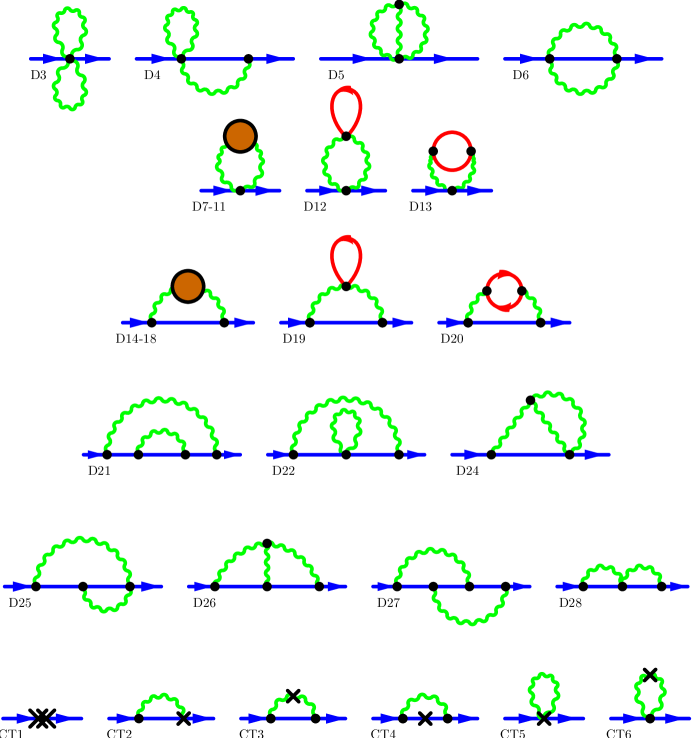
Figure 1: The two-loop diagrams that contribute to the pole-mass renormalization in the lattice scheme. The numbering is consistent with Ref. Panagop . The filled circles represent five one-loop sub-diagrams which dress the gluon propagator at that order (these contain gluon and ghost loops, and the measure term), in addition to the diagrams with internal-quark loops, which are shown explicitly. The quark-loop diagrams are understood to be summed over all flavors. The crosses represent vertices generated by the perturbative expansion of tadpole and other renormalization factors in the gluon and quark actions.

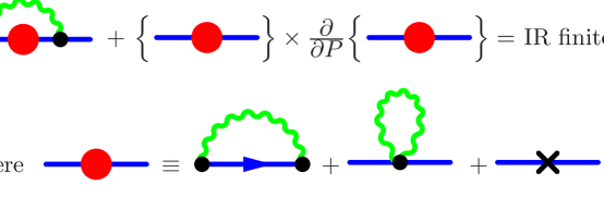
Figure 2: Schematic representation of an IR subtraction for the two-loop pole mass; appropriate traces of the self-energy with an energy projector are implicit.

Figure 3: The $n_{f}=0$ part of the two-loop pole mass $M^{(4)}$ for the “asqtad” action (in units of $\alpha_{\rm lat}^{2}$), for varying quark mass $m_{0}a$ (upper panel). The squares and crosses distinguish two independent sets of calculations, each one by a different author. The lower panel shows the results after subtracting the known logarithms in $M^{(4)}$, which yields the term $A_{20}$ in in Eq. (7).

Figure 4: Comparison of the loop-quark mass dependence of pole-mass renormalization factors, on the continuum side of the matching, and on the lattice side. The lattice calculation used $am_{\rm valence}=0.001$. The continuum function was taken from Ref. Broadhurst ; the solid lines are from analytic expressions for the associated limits, cf. Eq. (6)

II.4 Evaluation of the two-loop lattice self-energy

The renormalized pole mass $M$ is identified from the pole in the dressed-quark propagator $G(p,m_{0})$,

$$G(p,m_{0})^{-1}=i/\!\!\!\widehat{p}+m_{0}+\Sigma_{\rm tot}(p),$$ (13)

where $\Sigma_{\rm tot}$ is minus the usual 1PI two-point function. The two-loop diagrams contributing to $\Sigma_{\rm tot}$ in the lattice theory are shown in Fig. 1. The lattice-dispersion relation implied by $\widehat{p}$ will be kept as a general function of the lattice momentum $p$; for improved-staggered quarks, for instance, $a\widehat{p}_{\mu}=\sin(ap_{\mu})+\frac{1}{6}\sin^{3}(ap_{\mu})$. We make the spinor decomposition:

$$\Sigma_{\rm tot}(p)=\Sigma_{1}(p)+(i/\!\!\!\widehat{p}+m_{0})\,\Sigma_{2}(p),$$ (14)

where $\Sigma_{1}$ and $\Sigma_{2}$ are both implicit functions of $m_{0}$, and both are Dirac scalars. At zero three-momentum the renormalized on-shell condition is given by

$$P(p_{t})\equiv-i\widehat{p}_{t}=m_{0}+\frac{\Sigma_{1}(p)}{1+\Sigma_{2}(p)},$$ (15)

the solution of which determines the pole mass

$$p_{t}=iM.$$ (16)

The perturbative expansion of $M$ is denoted by

$$M=M^{(0)}+g_{0}^{2}M^{(2)}+g_{0}^{4}M^{(4)},$$ (17)

with a corresponding notation for other quantities (including, e.g., $p_{t}^{(0)}=iM^{(0)}$, where $P(iM^{(0)})=m_{0}$). At first order one has

$$M^{(2)}=Z_{\Psi}^{(0)}\,\Sigma_{1}^{(2)}(p^{(0)}),$$ (18)

where

$${Z_{\Psi}^{(0)}}^{-1}=\left.\frac{dP(ix)}{dx}\right|_{x=M^{(0)}},$$ (19)

is the tree-level wave function residue.

An evaluation of the on-shell condition to second order requires a consistent expansion of the right-hand side of Eq. (15). Part of the $O(g_{0}^{4})$ term arises from the one-loop piece of $\Sigma_{1}(p_{t})$, when it is evaluated at the one-loop-corrected on-shell energy

$$\Sigma_{1}^{(2)}(p_{t})\simeq\Sigma_{1}^{(2)}(iM^{(0)})+ig_{0}^{2}\,M^{(2)}\left.\frac{\partial\Sigma_{1}^{(2)}(p_{t})}{\partial p_{t}}\right|_{p_{t}=iM^{(0)}}.$$ (20)

Hence the two-loop contribution to the pole mass is given by

$$M^{(4)}=Z_{\psi}^{(0)}\left(m^{(4)}-{\textstyle{\frac{1}{2}}}(M^{(2)})^{2}{\left.\frac{d^{2}P(ix)}{dx^{2}}\right|_{x=M^{(0)}}}\right),$$ (21)

where

$$m^{(4)}=\Sigma_{1}^{(4)}(iM^{(0)})+\Sigma_{1}^{(2)}(iM^{(0)})\,{\Sigma_{\rm tot}^{(2)}}^{\,\prime}(iM^{(0)}),$$ (22)

with

$${\Sigma_{\rm tot}^{(2)}}^{\,\prime}(iM^{(0)})\equiv-\Sigma_{2}^{(2)}(iM^{(0)})+iZ_{\psi}^{(0)}\left.\frac{\partial\Sigma_{1}^{(2)}(p_{t})}{\partial p_{t}}\right|_{p_{t}=iM^{(0)}}.$$ (23)

Note that the second-term in Eq. (21) is a correction of $O((am_{0})^{3})$ in the continuum limit of the “asqtad” action.

The derivative ${\Sigma_{\rm tot}^{(2)}}^{\,\prime}$ of the one-loop self-energy (differentiation is implicitly defined in Eq. (23) as with respect to $P(p_{t})$) is also the one-loop part of the wave function renormalization (up to finite-lattice discretization corrections), and is infrared divergent. This infrared divergence precisely cancels against an infrared divergence in the two-loop nested-rainbow diagrams (the sum of D21, D22, and CT4 in Fig. 1), which parallels the cancellation of infrared divergences in the continuum self-energy at this order. In this connection, we note that the continuum-pole mass was first shown to be infrared finite at two loops in Ref. Tarrach ; an all-orders proof of its finiteness has been established only fairly recently, by Kronfeld Kronfeld .

Figure 2 illustrates the infrared cancellation in Eq. (22) in diagrammatic form. We numerically evaluate the two-loop integral for the left-hand diagram in the top line of Fig. 2 including, in its integrand, a term with the product of the independent integrands for the one-loop self-energy, and its derivative. This grouping is IR finite, and does not require any infrared regulator. We obtain a stringent check of this result by noting that this combination generates a leading-logarithmic contribution to the anomalous dimension of the mass which goes like $\log^{2}(am_{0})$, and whose coefficient is identical to that of the infrared-subtracted combination in the continuum, which can easily be read off in Feynman gauge from the $\overline{\text{MS}}$ results in Tarrach .

All the diagrams for the two-loop self-energy, Fig. 1, were generated and evaluated independently by two of us. The Feynman rules for the highly-improved actions are exceedingly complicated, and were generated automatically using computer-algebra based codes HReview ; QThesis . Moreover, one of us has produced an algorithm which automatically generates the Feynman diagrams themselves QThesis . We can then readily evaluate the lattice diagrams for a wide variety of gluon and quark actions. The two-loop integrals are evaluated numerically, using the adaptive Monte-Carlo method VEGAS Vegas . A powerful additional cross-check was provided by an explicit verification that our results are gauge independent, which we established numerically for two different bare-quark masses in three covariant gauges: Feynman, Landau and Yennie.

Knowing the coefficients of the logarithmic terms in Eq. (7) also provides a valuable cross-check on our results, and increases the accuracy of our numerical determination of the remaining term $A_{20}$. We compute the two-loop pole mass as a function of $m_{0}a$, and subtract the known logarithms, in order to isolate $A_{20}$, which must be finite as $m_{0}a\to 0$. Figure 3 shows the $n_{f}=0$ part of the results, corresponding to the diagrams without internal-fermion loops, over a wide range of bare masses, and clearly shows the expected limiting behavior.

Additional checks are provided for diagrams which have a leading $\log^{2}(am_{0})$ term, which arises from the infrared limit of both the outer- and inner-loop integrals, and which is therefore an infrared quantity, independent of the ultraviolet regulator; the coefficients of these double logarithms in the individual diagrams are available in Feynman gauge from the original two-loop $\overline{\text{MS}}$ calculation of Tarrach Tarrach , and we have verified that these are reproduced in our lattice calculation.

A further stringent check of our evaluation of the diagrams with fermion loops (diagrams 12, 13, 19 and 20 in Fig. 1) is achieved by computing over a range of sea quark masses. As discussed in Sect. II.3, the mass dependence in the intermediate renormalization from the bare mass to the pole mass $M$ should cancel against the renormalization from $M$ to the $\overline{\text{MS}}$ mass. We define

$$A_{20}(r_{\rm sea})\equiv A_{20}(0)+\frac{4}{3\pi^{2}}\Delta_{\rm lat}(r_{\rm sea}),$$ (24)

and compare with the analogous continuum function $\Delta(r_{\rm sea})$, cf. Eqs. (2)–(6). We plot our results in Fig. 4, over a very wide range in $r_{\rm sea}$, which shows the expected agreement.

Our result for the matching term $A_{20}$, in the limit of vanishing sea-quark mass, is

$$A_{20}=6.092(20)-0.1484(5)n_{\ell}-0.0328(3),$$ (25)

where the last term corresponds to an internal-quark loop containing the valence-quark flavor. The uncertainties arise from the numerical evaluation of the loop integrals.

The relatively large value of $A_{20}$ may be a symptom of the renormalon ambiguity Renormalon in the pole mass $M$; there is similarly a large second-order term in the connection between $M$ and the $\overline{\text{MS}}$ mass, Eq. (2). However, as seen in the next subsection, these large corrections in the intermediate matchings to the pole mass mostly cancel in the final matching of the bare mass to the $\overline{\text{MS}}$ mass, Eq. (1), for which perturbation theory should be (and is) reliable.

Figure 5: BLM scales $aq^{*}$ for the lattice-bare mass to $\overline{\text{MS}}$ mass matching factor $Z_{m}(\mu a)$, as functions of $\mu a$. The solid line shows the first-order scale $q_{1}^{*}$, while the dashed and dotted lines show the second-order scales $q_{2+}^{*}$ and $q_{2-}^{*}$, respectively, in regions where they are real. The first-order scale is the correct choice for $\mu a\lesssim 0.61$ and $\mu a\gtrsim 3.74$, while the appropriate second-order scale applies to the region in between.

II.5 Results for $Z_{m}$ and its BLM scale

To complete our determination of the matching factor $Z_{m}$ in Eq. (1) we substitute the expression Eq. (7) for the pole mass in the lattice scheme into the equivalent $\overline{\text{MS}}$ expression in Eq. (2), and expand the logarithms in powers of the coupling. We also reorganize the couplings to the $\alpha_{V}$ scheme at some scale $q^{*}$, which we determine below according to the BLM procedure BLM . This leaves an expression with logarithms only of $\mu a$ and $aq^{*}$. The logarithms of $m_{0}$ drop out of $Z_{m}$, as expected, since these are infrared effects that are identical in the intermediate lattice and continuum matchings. [We note that the coefficients of the logarithms in Eq. (7), corresponding to the lattice anomalous dimension, could instead be determined from the requirement that the logarithms of $m_{0}$ drop out of the final expression for $Z_{m}$.]

$Z_{m}$ then takes the form

$$Z_{m}(\mu a,m_{0}a)=1+Z_{m,1}(\mu a)\alpha_{V}\!\left(q^{*}(\mu a)\right)$$

$$+Z_{m,2}(\mu a)\alpha_{V}^{2}+\mathcal{O}\left(\alpha^{3},(m_{0}a)^{2}\right),$$ (26)

where the first-order term was derived previously in Ref. Hein

$$Z_{m,1}(\mu a)=0.1188(1)-\frac{2}{\pi}\log(\mu a).$$ (27)

The new information presented here is the expression for $Z_{m,2}(\mu a)$, which takes the form

$$Z_{m,2}(\mu a)=Z_{22}\log^{2}(\mu a)+Z_{21}\log(\mu a)+Z_{20},$$ (28)

wherre

$$Z_{22} =0.7599-0.0338\,n_{f},$$ (29)

$$Z_{21} =-0.4049-0.0281\,n_{f}$$

$$\ +(-1.1145+0.0675\,n_{f})\log(aq^{*}),$$ (30)

$$Z_{20} =2.086(20)-0.0144(5)n_{f}$$

$$\ +(0.2080-0.0126\,n_{f})\log(aq^{*}).$$ (31)

To find the optimal choice for $aq^{*}$ in the BLM scheme, as a function of $\mu a$, we analytically evaluated the average-momentum scales in the one-loop $\overline{\text{MS}}$ self-energy diagram (with appropriate renormalizations BLM ), and made numerical evaluations of the average scales in the lattice self-energy. We find that the second-order scale-setting procedure of Ref. BLM is needed over a wide range of scales in the region of $\mu a=1$.

At leading order the scale $q^{*}$ is determined by Viability ; BLM

$$\log(q_{1}^{*}{}^{2}) =\frac{\int d^{4}qf(q)\log(q^{2})}{\int d^{4}qf(q)}\equiv\frac{\langle f(q)\log(q^{2})\rangle}{\langle f(q)\rangle},$$

$$\equiv\langle\langle\log(q^{2})\rangle\rangle$$ (32)

where $f(q)$ is the integrand for the one-loop matching factor, that is, $\langle f(q)\rangle=Z_{m,1}(\mu a)$. We find

$$\langle f(q)\log(q^{2}a^{2})\rangle =-\frac{2}{\pi}\log^{2}(\mu a)-\frac{5}{3\pi}\log(\mu a)$$

$$\ \ -\frac{1}{2\pi}+\frac{5\pi}{12}-0.821$$ (33)

where the numerical constant is the result of the numerical evaluation of the lattice moment (logarithms of $m_{0}$ due to the anomalous dimension of the pole mass cancel in the scale for the matching coefficient).

When $|Z_{m,1}(\mu a)|$ is anomalously small, a proper evaluation of $q^{*}$ requires the second-order expression

$$\log(q_{2\pm}^{*2})=\langle\langle\log(q^{2})\rangle\rangle\pm\left[\langle\langle\log(q^{2})\rangle\rangle^{2}-\langle\langle\log^{2}(q^{2})\rangle\rangle\right]^{1/2},$$ (34)

where the appropriate root (if the result is real) is usually made obvious by requiring continuity, and a physically reasonable value, for the resulting $q^{*}$, as a function of the underlying parameters. The second moment of $Z_{m,1}$ is given by

$$\langle f(q)\log^{2}(q^{2}a^{2})\rangle=-\frac{8}{3\pi}\log^{3}(\mu a)-\frac{10}{3\pi}\log^{2}(\mu a)$$

$$\ \ +\frac{(\pi^{2}-9)}{3\pi}\log(\mu a)-\frac{5}{3\pi}-\frac{10\,\zeta_{3}}{3\pi}-\frac{7\pi}{36}+3.057.$$ (35)

Results for the first- and (where appropriate) second-order scales, as functions of $\mu a$, are shown in Fig. 5. A typical value is $aq^{*}=1.877$ at $\mu a=1$.

III Results for light-quark masses

The bare lattice masses for the strange and up/down quarks, on the MILC “coarse” and “fine” lattices, are given in Ref. OneLoopMass . For the strange quark these are $am_{0s}=0.0390(1)(20)/u_{0c}$, and $am_{0s}=0.0272(1)(12)/u_{0f}$, on the coarse and fine lattices respectively, where $u_{0c}=0.86774$ and $u_{0f}=0.87821$ are tadpole normalization factors. The uncertainties are lattice statistical and systematic errors, respectively, the latter due mainly to chiral extrapolation/interpolation. The lattice spacings can be found in Ref. HPQCDalphas , $a^{-1}_{\rm coarse}=1.596(30)$ GeV, and $a^{-1}_{\rm fine}=2.258(32)$ GeV.

Following conventional practice we quote the light-quark $\overline{\text{MS}}$ masses at the scale $\mu=2$ GeV, taking three active flavors of quarks ($n_{f}=3$). The BLM scales on the two MILC lattices are then $aq^{*}_{\rm coarse}=2.144$ and $aq^{*}_{\rm fine}=1.752$ CouplingNote . This results in two-loop coefficients in Eq. (26) of $Z_{m,2}|_{\rm coarse}=1.939(20)$, and $Z_{m,2}|_{\rm fine}=2.270(20)$. We also require the couplings at the relevant scales, and for this purpose we use the recently determined value $\alpha_{V}^{(n_{f}=3)}(7.5~{}\mbox{GeV})=0.2082(40)$ HPQCDalphas . We find $\alpha_{V}(q^{*}_{\rm coarse})=0.2925(92)$, and $\alpha_{V}(q^{*}_{\rm fine})=0.2713(76)$ CouplingNote .

Putting all of this together, we obtain the following values for the $\overline{\text{MS}}$ strange-quark mass, on the two lattices

$$m^{\text{$\overline{\text{MS}}$}}_{s}(2~{}\mbox{GeV}) =84(5)~{}\mbox{MeV\ [coarse]},$$

$$m^{\text{$\overline{\text{MS}}$}}_{s}(2~{}\mbox{GeV}) =86(4)~{}\mbox{MeV\ [fine]},$$ (36)

where the errors above are just from the simulation systematics; we note that these errors are correlated, because the two bare masses are obtained from a simultaneous-chiral fit to the two lattice spacings, which describes the effects of taste-changing and other discretization effects in the staggered action MILCchiral .

We consider continuum extrapolations of these values, based on the form of the expected leading-discretization errors, which are of $O(\alpha_{V}a^{2})$ (we find essentially identical results by assuming $O(\alpha_{V}^{2}a^{2})$ errors OneLoopMass ). In addition, we estimate the third-order perturbative correction to the matching factor, that is, we add a term $Z_{m,3}(\mu a)\alpha_{V}^{3}$ to the right-hand side of Eq. (26), and attempt to estimate its coefficient. To this end, we extend the lattice renormalization factor Eq. (7) to third order, including the logarithms from the three-loop anomalous dimension, which are fixed from the known $\overline{\text{MS}}$ expansion, along with the known third-order term in Eq. (2) for the $\overline{\text{MS}}$ mass Chetyrkin ; Melnikov . This leaves one unknown constant, in the lattice renormalization factor, $A_{30}$ in the notation of Eq. (7), which with the third-order logarithms determines $Z_{m,3}(\mu a)$. In principle, one can extract $A_{30}$, and hence the third-order correction, from a simultaneous fit using bare lattice masses at several lattice spacings; this extends a technique first laid out in Ref. HPQCDalphas (see also Ref. HighBeta ).

With only the two available lattice spacings, and having also to include a discretization correction in the fit, we can only roughly bound the size of the next order in the perturbative expansion. We used constrained curve-fitting Constrained ; HPQCDalphas to include our expectation that the expansion is convergent (i.e., $|Z_{m,3}(\mu a)|=O(1)$ in the notation of Eq. (26)).

We tested this procedure by considering a fit to the second-order perturbative correction $Z_{m,2}(\mu a)$, without a priori knowledge of the associated constant $A_{20}$: with the two lattice spacings as input, and including a discretization correction, the fit returns $A_{20}=5.9\pm 1.9$, in good agreement with Eq. (25). The second-order fit also returns $m_{s}^{\text{$\overline{\text{MS}}$}}(2~{}\mbox{GeV})=(85\pm 11)$ MeV, in good agreement with the “bona-fide” two-loop values in Eq. (36) [this also represents somewhat of an improvement compared to our earlier result OneLoopMass , which used only a priori first-order perturbation theory, without a fit to the second-order correction, and which somewhat underestimated both the central value and the systematic error from the truncation of the perturbative series].

When this procedure is applied at third-order, with $A_{20}$ input from Eq. (25), the fit provides a reasonable estimate of the relative systematic error on the $\overline{\text{MS}}$ mass, due to the third-order perturbative correction, of approximately $2\times\alpha_{V}^{3}$, or about 4% (there is no appreciable third-order correction to the $\overline{\text{MS}}$ mass, within this error). We also use these fits (which include a discretization correction) to extract the central value of the strange-quark mass. Our final value is then

$$m^{\text{$\overline{\text{MS}}$}}_{s}(2~{}\mbox{GeV})=87(0)(4)(4)(0)~{}\mbox{MeV}$$ (37)

where, following Ref. OneLoopMass , the respective errors are statistical, lattice systematic, perturbative, and electromagnetic/isospin effects.

Our result for the ratio of the strange-quark mass to the up/down-quark masses is unchanged from Ref. OneLoopMass , since the renormalization factor is mass independent, as we have verified explicitly in Sect. II through two-loops (and up to a negligible mass-dependent discretization correction)

$$\frac{m_{s}}{\hat{m}}=27.4(1)(4)(0)(1),$$ (38)

where $\hat{m}\equiv\frac{1}{2}(m_{u}+m_{d})$. Equivalently we have

$$\hat{m}^{\text{$\overline{\text{MS}}$}}(2~{}\mbox{GeV})=3.2(0)(2)(2)(0)~{}\mbox{MeV}$$ (39)

Using a recent determination of the ratio $m_{u}/m_{d}=0.43(0)(1)(0)(8)$ due to the MILC collaboration MILCmud , these results imply

$$m^{\text{$\overline{\text{MS}}$}}_{u}(2~{}\mbox{GeV}) =1.9(0)(1)(1)(2)~{}\mbox{MeV},$$

$$m^{\text{$\overline{\text{MS}}$}}_{d}(2~{}\mbox{GeV}) =4.4(0)(2)(2)(2)~{}\mbox{MeV}.$$ (40)

IV Discussion and Conclusions

Perturbation theory has once again shown itself to be an essential tool in high-precision phenomenological calculations from the lattice. The two-loop lattice diagrams for the renormalized-quark mass were conquered with a combination of algebraic and numerical techniques in this first-ever two-loop evaluation of a multiplicative “kinetic” mass on the lattice. When combined with the known continuum matching from the pole mass to the $\overline{\text{MS}}$ mass, a very accurate determination of the light-quark masses was possible. The results presented here have a number of distinguishing features: two-loop perturbation theory; $n_{f}=2+1$ simulations with two degenerate light quarks and a heavier strange quark; very small light quark masses from $m_{s}/8$ to $m_{s}/2$ which enabled a partially quenched chiral fit with many terms to thousands of configurations; and extremely accurate determinations of the lattice spacings, which are equal within small errors when set from any of a wide variety of hadronic inputs.

Most notable amongst our results is our new value for strange quark mass, $m^{\text{$\overline{\text{MS}}$}}_{s}(2~{}\mbox{GeV})=87(0)(4)(4)(0)~{}\mbox{MeV}$, where the respective errors are lattice statistical, lattice systematic (mostly due to the chiral extrapolation/interpolation), perturbative, and due to electromagnetic/isospin effects. The two-loop matching has increased the central value of our estimates of the light-quark masses with respect to our previous one-loop determination OneLoopMass by about 1.5 standard deviations, based on the previous estimate of the perturbation-theory uncertainty. The systematic uncertainty from perturbation theory has been reduced by about a factor of two, and is now only about 4%, the same size as the current lattice systematic uncertainty, the latter due mainly to the chiral extrapolation/interpolation. We anticipate that the present estimate of the perturbative uncertainty could be reduced somewhat further, if additional lattice spacings become available, by using the NNLO perturbation theory presented here to improve the estimate of the third-order perturbative correction, along the lines that we have implemented above.

The strange-quark mass determination has historically generated some controversy, with widely different values having been obtained from different approaches. This is reflected in the large uncertainty in the Particle Data Group’s most recent best estimate, $m^{\text{$\overline{\text{MS}}$}}_{s}(2~{}\mbox{GeV})=(105\pm 25)$ MeV PDG ; our result represents a significant improvement in precision, resulting from an aggressive effort to understand and reduce all sources of systematic error.

An obvious advantage of our result is that it has been obtained with the correct description of the sea, that is, with $n_{f}=2+1$ flavors of dynamical quarks. There is only one other three-flavor result, which is due to the CP-PACS and JLQCD collaborations (which did simulations at much larger $u/d$ quark masses than in the MILC “asqtad” ensembles), which recently reported a value of $m^{\text{$\overline{\text{MS}}$}}_{s}(2~{}\mbox{GeV})=87(6)$ MeV CPPACS-JLQCD ; however they do not include a full error analysis, and in particular the error from missing higher orders in the perturbative matching alone should be comparable to that in our older result, and significantly larger than the errors that we report here with a 2-loop analysis.

It appears that the most recent estimates of the strange-quark mass extracted from simulations with only two flavors of sea quarks are systematically higher than the estimates with the correct $n_{f}$, although the other systematic errors are too large to allow for a definitive assessment (noting that these two-flavor determinations were also done with different definitions of the quark mass and determinations of the lattice spacing from $r_{0}$ using different physical values for $r_{0}$). The two-flavor determination from the QCDSF-UKQCD collaboration is $m^{\text{$\overline{\text{MS}}$}}_{s}(2~{}\mbox{GeV})=100-130$ MeV QCDSF-UKQCD , the ALPHA collaboration value is $97(22)$ MeV ALPHA , and the Rome value is $101(8)\binom{\scriptstyle+25}{\scriptstyle-9}$ MeV Rome . In this connection, we analyzed quenched simulations of the “asqtad” action by the MILC collaboration MILCsims ; MILCchiral , and we find that this also leads to a somewhat larger value of the strange quark mass, of about 96 MeV quenched (using simple linear interpolations of the MILC quenched-meson spectrum results, and our two-loop perturbative matching formula at $n_{f}=0$).

We are currently in the process of applying our NNLO matching calculation to heavy-quark masses, in order to complete a high-precision determination of the fundamental parameters of QCD. Work is also underway on the NNLO matching calculations for important hadronic matrix elements, especially those such as the decay constants $f_{D}$ and $f_{B}$ and other form-factors of particular relevance to heavy-flavor physics.

- (1) G. P. Lepage and P. B. Mackenzie, Phys. Rev. D 48, 2250 (1993)
- (2) G. P. Lepage, Phys. Rev. D 59, 074502 (1999).
- (3) K. Orginos and D. Toussaint, Phys. Rev. D 59, 014501 (1999); C. W. Bernard et al., MILC Collaboration, Phys. Rev. D 64, 054506 (2001)
- (4) W. J. Lee and S. R. Sharpe, Phys. Rev. D 60, 114503 (1999); C. Aubin and C. Bernard, Phys. Rev. D 68, 034014 (2003)
- (5) C. Aubin et al., MILC Collaboration, Phys. Rev. D 70, 094505 (2004).
- (6) C. T. H. Davies et al., HPQCD, Fermilab and MILC Collaborations, Phys. Rev. Lett. 92 022001 (2004).
- (7) H. D. Trottier, Nucl. Phys. Proc. Suppl. 129, 142 (2004).
- (8) Q. J. Mason, Ph.D. thesis, Cornell University (2004).
- (9) Q. Mason et al., HPQCD Collaboration, Phys. Rev. Lett. 95 (2005) 052002.
- (10) E. Follana and H. Panagopoulos, Phys. Rev. D 63 (2000) 017501.
- (11) U. M. Heller and F. Karsch, Nucl. Phys. B 251, 254 (1985); G. Martinelli and C. T. Sachrajda, Nucl. Phys. B 559, 429 (1999).
- (12) A. Gray et al., HPQCD Collaboration, hep-lat/0507013.
- (13) C. Aubin et al., HPQCD, MILC, and UKQCD Collaborations, Phys. Rev. D. 70 (2004) 031504.
- (14) J. Hein, Q. Mason, G. P. Lepage and H. Trottier, Nucl. Phys. Proc. Suppl. 106, 236 (2002).
- (15) W. J. Lee and S. R. Sharpe, Phys. Rev. D 66, 114501 (2002).
- (16) Q. Mason and H. D. Trottier, in preparation.
- (17) E. Follana, A. Hart and C. T. H. Davies, Phys. Rev. Lett. 93, 241601 (2004); K. Y. Wong and R. M. Woloshyn, Phys. Rev. D 71, 094508 (2005); S. Durr, C. Hoelbling and U. Wenger, Phys. Rev. D 70, 094502 (2004).
- (18) Q. Mason et al., HPQCD collaboration, Nucl. Phys. Proc. Suppl. 119, 446 (2003); E. Follana et al., HPQCD Collaboration, ibid., 129 & 130, 384 (2004).
- (19) R. Tarrach, Nucl. Phys. B 183, 384 (1981).
- (20) N. Gray, D. J. Broadhurst, W. Grafe and K. Schilcher, Z. Phys. C 48, 673 (1990); D. J. Broadhurst, N. Gray and K. Schilcher, ibid. 52, 111 (1991).
- (21) K. G. Chetyrkin and M. Steinhauser, Nucl. Phys. B 573, 617 (2000).
- (22) K. Melnikov and T. v. Ritbergen, Phys. Lett. B 482 (2000) 99.
- (23) Q. Mason, H. D. Trottier, R. Horgan, hep-lat/0510053.
- (24) Y. Schröder, Phys. Lett. B 447, 321 (1999)
- (25) A. S. Kronfeld, Phys. Rev. D 58, 051501 (1998).
- (26) G. P. Lepage, J. Comput. Phys. 27 (1978) 192.
- (27) For a review see, e.g., M. Beneke, Phys. Rept. 317, 1 (1999).
- (28) S. J. Brodsky, G. P. Lepage and P. B. Mackenzie, Phys. Rev. D 28, 228 (1983); K. Hornbostel, G. P. Lepage and C. Morningstar, Phys. Rev. D 67, 034023 (2003).
- (29) The values of the scales used here are more accurate than the slightly larger values given in Ref. OneLoopMass , where an approximate determination was made of the average-loop momentum circulating in the continuum self-energy. In addition an earlier, approximate (and somewhat smaller), determination of was employed in Ref. OneLoopMass .
- (30) H. D. Trottier, N. H. Shakespeare, G. P. Lepage and P. B. Mackenzie, Phys. Rev. D 65, 094502 (2002).
- (31) G. P. Lepage et al., Nucl. Phys. Proc. Suppl. 106, 12 (2002)
- (32) C. Aubin et al., MILC collaboration, Phys. Ref. D 70, 114501 (2004).
- (33) S. Eidelman et al., Particle Data Group, Phys. Lett. B 592, 1 (2004).
- (34) T. Ishikawa et al., CP-PACS and JLQCD collaborations, hep-lat/0509142.
- (35) M. Gockeler et al., QCDSF-UKQCD collaboration, hep-lat/0509159.
- (36) M. Della Morte et al., ALPHA collaboration, hep-lat/0509073.
- (37) D. Becirevic et al., hep-lat/0509091.