We address the nonperturbative effects associated with soft charm quarks in inclusive $B$ decays. Such corrections are allowed by the OPE, but have largely escaped attention so far. The related four-quark ‘double heavy’ expectation values of the form $\langle B|\bar{b}c\,\bar{c}b|B\rangle$ are computed in the $1/m_{c}$ expansion by integrating out the charm field to one and two loops. A significant enhancement of the two-loop coefficients is noted. A method is suggested for evaluating the expectation values of the higher-order $b$-quark operators required to calculate charm expectation values, free from the overly large ambiguities of dimensional analyses. The soft-charm effects were found generally at the level of $0.5\%$ in $\Gamma_{\rm sl}(b\!\to\!c)$; our literal estimate is somewhat smaller as a result of partial cancellations. We propose a direct way to search for such effects in the data. Finally, we discuss the relation of the soft charm corrections in inclusive decays with the ‘Intrinsic Charm’ ansatz.

^∗ On leave of absence from St. Petersburg Nuclear Physics Institute, Gatchina, St. Petersburg 188300, Russia

1 Introduction

Inclusive weak or radiatively induced electroweak decay rates of heavy flavor, in particular of beauty hadrons can be rigorously treated in the heavy quark expansion employing a local operator expansion in powers of $1/m_{Q}$ (OPE). For fully integrated rates there are no nonperturbative corrections scaling like $1/m_{Q}$ [1, 2], and the leading contributions are given to order $1/m_{b}^{2}$ in terms of the expectation values of the kinetic and chromomagnetic heavy quark operators. They incorporate effects due to bound-state dynamics in the initial state as well as the propagation of the hard final state quarks through the nonperturbative hadronic medium during the decay. In this respect they are analogous to the leading power correction in the vacuum current correlator due to the gluon condensate $\propto\frac{\langle G^{2}\rangle}{Q^{4}}$ [3].

At order $1/m_{b}^{3}$ four-quark operators of the form $\langle B|\bar{b}\Gamma q\,\bar{q}\Gamma b|B\rangle$ appear in the expansion of the decay rates. They describe, for instance, weak annihilation (or weak scattering in baryons) and Pauli interference which distinguish the decays of hadrons with different flavors of the light spectator quarks – yet they generate flavor-singlet effects as well. Their meaning is transparent: the propagation of soft light quarks in the decay is not perturbative, neither literally nor in the duality sense, and the overall contribution from these kinematics should be regarded as an additional nonperturbative input [4, 5]. It parallels the quark condensate effect in the vacuum correlator [3].

Inclusive semileptonic $B$ decays offer the cleanest theoretical environment for precision application of the OPE. They allow to extract both the heavy quark parameters $m_{b}$, $m_{c}$, $\mu_{\pi}^{2}$ etc. and $|V_{cb}|$ or $|V_{ub}|$ with (almost) unmatched  accuracy (see, for instance, Ref. [7]). It is then essential to analyze all contributions, even small ones [8].

The four-fermion operator $\bar{b}\gamma_{k}(1\!-\!\gamma_{5})u\,\bar{u}\gamma^{k}(1\!-\!\gamma_{5})b$ explicitly appears at tree level in the semileptonic $b\!\to\!u$ decays [5]. In the dominant semileptonic mode $b\!\to\!c$ analogous contributions from $\bar{b}\gamma_{k}(1\!-\!\gamma_{5})c\,\bar{c}\gamma^{k}(1\!-\!\gamma_{5})b$ are usually neglected under the tacit assumption that $c$ quarks are sufficiently heavy as not to induce nonperturbative effects. This assumption is valid only up to a point: nonperturbative charm effects could a priori become relevant at the one percent level.

There is a complementary reason to introduce explicitly the four-quark expectation values with the charm quark fields, which becomes manifest once the heavy quark expansion in $b\!\to\!c\,\ell\nu$ is extended beyond order $1/m_{b}^{3}$. For instance, in calculating $\Gamma_{\rm tot}$ we expand the charm quark Green function in the external field. Similar to differentiating over $m_{c}^{2}$, this produces increasingly infrared-sensitive integrals converging at $k_{c}\lower 3.01385pt\hbox{$\;\stackrel{{\scriptstyle\textstyle<}}{{\sim}}\;$}m_{c}$ rather than at the hard scale of the energy release. Consequently, the resulting expansion in general includes terms scaling like

$$\Gamma_{0}\,\mu_{\rm hadr}^{k+l}\,\frac{1}{m_{b}^{k}}\,\frac{1}{m_{c}^{l}}$$ (1)

with $l\!>\!0$ for $k\!\geq\!3$. Just for the above reasons these terms describe precisely the lump effect of the expectation values like $\langle B|\bar{b}\Gamma c\,\bar{c}\Gamma b|B\rangle$. Including the latter explicitly allows to preserve the principal advantage of the OPE for the inclusive rates, viz. expansion in $1/m_{b}$ (or, more generally, in the inverse energy release) free from corrections suppressed only by the inverse charm mass.

Therefore, with the charm quark significantly lighter than the $b$ quark and only marginally heavy on the QCD mass scale, it is advantageous to explicitly introduce the four-quark operators with charm into the OPE and analyze their impact.

The remainder of the paper will be organized as follows. In Sect. 2 the framework is set up which is then used to compute the charm expectation values in the $1/m_{c}$ expansion to one- and two-loop level. The expectation values of the $b$-quark operators of dimension $7$ and $8$ are estimated, and the contributions to $\Gamma_{\rm sl}(b\!\to\!c)$ from both $1/m_{c}^{2}$ and $\alpha_{s}/m_{c}$ terms are evaluated. In Sect. 3 we discuss the phenomenology of the soft-charm effects and point out that the $q^{2}$-moments of the decay distributions are rather sensitive to them. In Sect. 4 we summarize our conclusions and dwell on a possible connection of these effects with ‘Intrinsic Charm’ in $B$ particles. Appendices guide through technical details of our analysis: the conventions are described in Appendix A, the master technique for calculation is briefly reviewed in Appendix B and in Appendix C we describe the main steps in the technically challenging two-loop calculations.

2 The framework

The total semileptonic $b\!\to\!c$ decay rate in the OPE is given by

$$\Gamma_{\rm sl}(b\!\to\!c)\mbox{~{}} = \mbox{~{}}\frac{G_{F\,}^{2}m_{b}^{5}(\mu)}{192\,\pi^{3}}\;\raisebox{-1.42262pt}{\mbox{{\large$|V_{cb}|^{2}$}}}\,\left(1\!+\!A_{\rm ew}\right)\left[z_{0}(r)\,(1\!+\!A_{3}^{\rm pert}(r;\mu))\!\left(1\!-\!\frac{\mu_{\pi}^{2}(\mu)\!-\!\mu_{G}^{2}(\mu)\!+\!\frac{\rho_{D}^{3}(\mu)\!+\!\rho_{LS}^{3}(\mu)}{m_{b}(\mu)}}{2m_{b}^{2}(\mu)}\right)\right.$$ (2)

$$- \mbox{~{}}\left.(1+A_{5}^{\rm pert}(r;\mu))\,2(1\!-\!r)^{4}\frac{\mu_{G}^{2}(\mu)\!-\!\frac{\rho_{D}^{3}(\mu)\!+\!\rho_{LS}^{3}(\mu)}{m_{b}(\mu)}}{m_{b}^{2}(\mu)}+(1+A_{D}^{\rm pert})d(r)\,\frac{\rho_{D}^{3}(\mu)}{m_{b}^{3}(\mu)}\right.$$

$$+ \mbox{~{}}\left.32\pi^{2}\,(1+A_{6c}^{\rm pert}(r))(1\!-\!\sqrt{r})^{2}\frac{H_{c}}{m_{b}^{3}(\mu)}+32\pi^{2}\,\tilde{A}_{6c}^{\rm pert}(r)(1\!-\!\sqrt{r})^{2}\frac{\tilde{H}_{c}}{m_{b}^{3}(\mu)}\right.$$

$$+ \mbox{~{}}\left.32\pi^{2}A_{6q}^{\rm pert}(r)\frac{F_{q}}{m_{b}^{3}(\mu)}+{\cal O}\left(\frac{1}{m_{b}^{4}}\right)\right].\qquad\qquad$$

The coefficients $A_{i}^{\rm pert}$ stand for perturbative $\alpha_{s}$ corrections and $r=(m_{c}/m_{b})^{2}$,

$$z_{0}(r)\mbox{~{}} = \mbox{~{}}1-8r+8r^{3}-r^{4}-12r^{2}\ln{r}\;,$$

$$d(r)\mbox{~{}} = \mbox{~{}}8\ln{r}+\frac{34}{3}-\frac{32}{3}r-8r^{2}+\frac{32}{3}r^{3}-\frac{10}{3}r^{4}\;.$$ (3)

A detailed discussion can be found in Ref. [8]. We have adopted the Wilsonian prescription of introducing an auxiliary scale $\mu$ to separate large- and short-distance dynamics consistently.

The last term in Eq. (2) proportional to $F_{q}$ denotes the effect of generic $SU(3)$-singlet four-quark operators (other than Darwin operator) of the form $\bar{b}\Gamma b\>\bar{q}\Gamma q$ with the sum over $q=u,d,s$, and $\Gamma$ including both color and Lorentz matrices (to the leading order in $1/m_{b}$ only $\gamma_{0}\times\gamma^{0}$ or $\gamma_{i}\gamma_{5}\times\gamma^{i}\gamma_{5}$ structures survive, but one does not need to rely on this). Their Wilson coefficients are ${\cal O}(\alpha_{s})$, and we neglect these contributions.

Since the $b$ quark is sufficiently heavy, we consider terms only through order $1/m_{b}^{3}$. This includes the four-quark operators with the charm fields, yet only those without derivatives – the latter appear to order $1/m_{b}^{4}$ or higher. Without perturbative loop corrections only

$$H_{c}=\frac{1}{2M_{B}}\langle B|\bar{b}\gamma_{\nu}(1\!-\!\gamma_{5})c\,\bar{c}\gamma^{\rho}(1\!-\!\gamma_{5})b|B\rangle_{\mu}\>\left(-\delta^{\nu}_{\rho}\!+\!v^{\nu}v_{\rho}\right)\,,\qquad v_{\nu}=\frac{P^{B}_{\nu}}{M_{B}}$$ (4)

will contribute. This form literally implies the demarcation point $\mu$ to be above the $c$ quark mass, in which case charm is fully dynamical. The four-quark expectation values then are dominated by the large perturbative piece $\propto\mu^{3}/6\pi^{2}$. It is natural to eliminate it by evolving the theory down to smaller $\mu$ and eventually integrating out the charm field. This procedure adds nonperturbative corrections to be analyzed below.

Limiting ourselves to the third order in $1/m_{b}$ – the leading one for these operators – amounts to treating them in the static limit $m_{b}\!\to\!\infty$. There are then in general four $O(3)$-invariant parity-conserving operators possible of the form $\bar{b}b\,\bar{c}\gamma_{0}c$ and $\bar{b}\vec{\sigma}b\,\bar{c}\vec{\gamma}\gamma_{5}c$, with two color contraction schemes each. In the actual semileptonic decays a certain combination enters which can be decomposed into color-singlet and color-octet operators in the $s$-channel:

$$H_{c}=\langle O_{1}^{c}\rangle \mbox{~{}}=\mbox{~{}} -\frac{1}{2M_{B}}\langle B|\bar{b}\gamma_{i}(1-\gamma_{5})c\,\bar{c}\gamma^{i}(1-\gamma_{5})b|B\rangle$$

$$F_{c}=\langle O_{2}^{c}\rangle \mbox{~{}}=\mbox{~{}} -\frac{1}{2M_{B}}\langle B|\bar{b}\mbox{$\frac{\lambda^{a}}{2}$}\gamma_{i}(1-\gamma_{5})c\,\bar{c}\mbox{$\frac{\lambda^{a}}{2}$}\gamma^{i}(1-\gamma_{5})b|B\rangle\;.\qquad$$ (5)

At a high normalization point only $H_{c}$ enters at tree level according to Eq. (2), however strictly speaking these two mix under renormalization. For our analysis we consider, in general, the four operators

$$O_{V}^{s}=\bar{b}b\,\bar{c}\gamma_{0}c\mbox{\hskip 19.91692pt~{}} O_{A}^{s}=\bar{b}\vec{\sigma}b\,\bar{c}\vec{\gamma}\gamma_{5}c$$

$$O_{V}^{o}=\bar{b}\mbox{$\frac{\lambda^{a}}{2}$}b\,\bar{c}\mbox{$\frac{\lambda^{a}}{2}$}\gamma_{0}c O_{A}^{o}=\bar{b}\mbox{$\frac{\lambda^{a}}{2}$}\vec{\sigma}b\,\bar{c}\mbox{$\frac{\lambda^{a}}{2}$}\vec{\gamma}\gamma_{5}c,\qquad$$ (6)

which emerge after Fierz reordering of the operators in Eq. (5):

$$O_{1}^{c} \mbox{~{}}=\mbox{~{}} -\frac{3}{2N_{c}}O_{V}^{s}+\frac{1}{2N_{c}}O_{A}^{s}-3O_{V}^{o}+O_{A}^{o}$$

$$O_{2}^{c} \mbox{~{}}=\mbox{~{}} -\frac{3}{4}(1-\mbox{$\frac{1}{N_{c}^{2}}$})O_{V}^{s}+\frac{1}{4}(1-\mbox{$\frac{1}{N_{c}^{2}}$})O_{A}^{s}+\frac{3}{2N_{c}}O_{V}^{o}-\frac{1}{2N_{c}}O_{A}^{o}\;.$$ (7)

We therefore have vector and axial currents of $c$ quarks created at the origin (the position of the $b$ quark); both can be color singlet or octet.

For sufficiently heavy charm quarks we can integrate them out from the theory and have an expansion of $H_{c}$ and $F_{c}$ (or, in general, for all the four operators in Eq. (7)) in terms of the local $b$ quark operators $o_{k}$ containing only gluon and light quark fields:

$$\langle O^{c}_{j}\rangle=\sum_{k}C_{jk}(\mu)\frac{1}{2M_{B}}\frac{\langle B|\bar{b}o_{k}b(0)|B\rangle_{\mu}}{m_{c}^{d_{k}-3}}\;,$$ (8)

where $d_{k}\!\geq\!3$ denote the dimension of the operators $o_{k}$. This series is an expansion in inverse powers of charm quark mass.

2.1 Integrating out the charm quarks

To integrate out charm quarks from the operators in Eq. (6) we calculate the one-loop as well as the two-loop (one hard gluon exchange) contributions. The latter are of the leading power in $1/m_{c}$, however contain an extra power of the running coupling $\alpha_{s}$.

2.1.1 One-loop expansion

The operators in Eqs. (6) can generically be written as

$$J_{12}\equiv\bar{b}\Gamma_{\!1}b\>\bar{c}\Gamma_{\!2}c\;;$$ (9)

to one loop order the dependence on $\Gamma_{\!1,2}$ totally factorizes when the charm field is integrated out. Without hard gluon corrections the expansion (8) reduces to the charm quark current in an external gluon field. In the notation of Eq. (9)

$$J_{12}=\bar{b}\,\Gamma_{1}\langle\bar{c}\Gamma_{2}c\rangle_{A}b\;;$$ (10)

where the average denotes the gluonic operator obtained from the charm Green function in the given external gauge field $A$. The required expectation values are then given by the averages of these composite operators over the $B$ meson states.

In practice we use the well-elaborated Fock-Schwinger gauge method, which yields the result directly in terms of gauge-covariant objects. Here we shall only state the results.  The method is briefly described in Appendix B and discussed in more detail in [10].

The absence of the $b$ quark when calculating $\langle\bar{c}\Gamma_{\!2}c\rangle_{A}$ brings in additional symmetries and simplifies the possible structure of the operators in the expansion. Lorentz and gauge invariance ensure that the lowest possible operators are of the general form $DGG$, with $D$ the covariant derivatives and $G$ the gluon field strength. Therefore these operators are of order $1/m_{c}^{2}$. They agree with the results presented in Ref. [9]. The vector color-singlet current emerges only at the higher order $1/m_{c}^{4}$.

In what follows we will mostly use the matrix representation; the covariant derivative $D_{\mu}\!=\!\partial_{\mu}\!-\!iA_{\mu}$ then acts as a commutator. This sometimes will be assumed and not written explicitly. More definitions can be found in Appendix A.

Axial current

For the axial current with arbitrary color we get to order $1/m_{c}^{2}$:

$$({\cal A}_{\mu})^{ba}\equiv\langle\bar{c}^{a}\gamma_{\mu}\gamma_{5}c^{b}\rangle_{A}=\frac{1}{48\pi^{2}m_{c}^{2}}\,\left(2\{[D_{\alpha},G^{\alpha\beta}],\tilde{G}_{\mu\beta}\}+\{[D_{\alpha},\tilde{G}_{\mu\beta}],G^{\alpha\beta}\}\right)^{ba}\>,$$ (11)

where $a$ and $b$ are fundamental (spinor) indices in the $SU(3)$ color space. Note that $[D_{\alpha},G^{\alpha\beta}]$ in the first term reduces to the color quark current, $g_{s}^{2}\sum_{q}\bar{q}\gamma_{\beta}q$ in the adjoint representation. For a spatial Lorentz index $i$ we can write

$$({\cal A}_{i})_{ba}=\frac{1}{48\pi^{2}m_{c}^{2}}\,\left(2\{[D_{i},B_{k}],E_{k}\}+\{[D_{i},E_{k}],B_{k}\}-\{[D_{k},B_{i}],E_{k}\}+\{[D_{k},E_{k}],B_{i}\}-\right.$$

$$\left.\mbox{\hskip 227.62204pt~{}}\epsilon_{ikl}[D_{0},E_{k}],E_{l}\}\right)_{ba}\;.$$ (12)

The application to the semileptonic decays does not require singling out the color-singlet piece of the current, and the obtained general expression appears most convenient. The case of the color singlet axial current corresponds to taking the trace over the color indices; it results in a much simpler equation:

$$A_{\mu}^{s}\equiv{\rm Tr}[{\cal A}]\equiv\langle\bar{c}^{a}\gamma_{\mu}\gamma_{5}c^{a}\rangle_{A}=\frac{1}{24\pi^{2}m_{c}^{2}}\,\partial_{\alpha}\,{\rm Tr}\,G^{\alpha\nu}\tilde{G}_{\mu\nu}$$ (13)

The axial singlet current has been calculated in Ref. [11]. Assuming that $\mu\!=\!i$ is a spatial index, the singlet current can be rewritten in the form

$$\partial_{\alpha\,}{\rm Tr}\,G^{\alpha\nu}\tilde{G}_{i\nu}=2\,\partial_{i\,}{\rm Tr}\,(\vec{E}\vec{B})-\partial_{k\,}({\rm Tr}\,E_{k}B_{i}-{\rm Tr}\,E_{i}B_{k})\>.$$ (14)

The expression for the general axial current can be cross-checked [10] via the non-Abelian axial anomaly using the expansion of the pseudoscalar density.

Vector current

For the most general color vector current we get

$$({\cal V}_{\mu})_{ba}\equiv\langle\bar{c}^{a}\gamma_{\mu}c^{b}\rangle_{A}=\frac{i}{240\pi^{2}m_{c}^{2}}\,\left(13[D_{\beta},[G_{\alpha\mu},G^{\alpha\beta}]]+8i([D^{\alpha},[D^{\beta},[D_{\beta},G_{\alpha\mu}]]]\right.$$

$$\left.\mbox{\hskip 113.81102pt~{}}-4i[D^{\beta},[D^{\alpha},[D_{\beta},G_{\alpha\mu}]]]\right)_{ba}\;.$$ (15)

It is readily verified that this current is covariantly conserved, $D^{\mu}{\cal V}_{\mu}\!=\!0$ [10] as required by gauge invariance. Note that we have dropped the leading term $D^{\nu}G_{\nu\mu}\!=\!g_{s}^{2}\sum_{q}\bar{q}\gamma_{\mu}q$ with a coefficient $\propto\!\ln{\frac{\Lambda^{2}_{\rm UV}}{m_{c}^{2}}}$, since it is accounted for in the Darwin operator in the width at order $\frac{1}{m_{b}^{3}}\frac{1}{m_{c}^{0}}$. The pure octet component of the current can be obtained by varying the gauge field effective action with respect to $A^{d}_{\mu}$ which yields ${\rm Tr}\,({\cal V}_{\mu}t^{d})$; this is explicitly verified in [10]. By setting $\mu\!=\!0$ – the only component surviving the static limit of the $b$ quarks – we can write the expression for the current as

$$({\cal V}_{0})_{ba}=13\left(D\!\cdot\!(E\!\times\!B)+D\!\cdot\!(B\!\times\!E)\right)+4i(2D_{\nu}D^{\beta}-D_{\nu}D^{\beta})D_{\beta}E_{k})$$ (16)

(here the usual commutators are assumed when we symbolically write products of covariant derivatives).

The vector color-singlet current vanishes at order $1/m_{c}^{2}$ as follows from an explicit calculation. This was anticipated in Ref. [11] based on $C$-parity arguments. The leading term appears at order $1/m_{c}^{4}$ and has the general form $DGGG$. This current describes the effective local interaction of the photon with the gluon fields (in the vacuum) due to heavy quarks, and is of independent interest. It can be written as a total derivative:

$${\cal V}^{s}_{\mu}\equiv\langle\bar{c}^{a}\gamma_{\mu}c^{a}\rangle_{A}=-\frac{1}{1440\pi^{2}m_{c}^{4}}\,\partial^{\alpha}\left(14\{G_{\alpha\beta}G^{\beta\gamma}G_{\gamma\mu}\}_{d}+5\{G_{\gamma\beta}G^{\beta\gamma}G_{\alpha\mu}\}_{d}\right)\;,$$ (17)

where $\{\dots\}_{d}$ means that the symmetric matrix product $\sim d_{abc}$ of the three matrices must be taken. This expression vanishes for the $SU(2)$ gauge group, as expected from $G$-parity [11, 10]. Gauge invariance ensures this current to be conserved, $\partial^{\mu}{\cal V}^{s}_{\mu}\!=\!0$, which is evident from the symmetry properties of the field strength tensors. The two terms, however, do not vanish for the Abelian $U(1)$ group; they can be obtained from the Euler-Heisenberg effective action as a variation with respect to the gauge field [10]. Eq. (17) therefore represents the minimal non-Abelian extension of the Abelian current. Once again anticipating that $\mu\!=\!0$ in the expectation values, the two terms above can be written as

$${\cal V}^{s}_{0}=\partial^{\alpha}(14\{G_{\alpha\beta}G^{\beta\gamma}G_{\gamma 0}\}_{d} + 5\{G_{\gamma\beta}G^{\beta\gamma}G_{\alpha 0}\}_{d})=$$ (18)

$$\partial_{a}\{4(E_{a}E^{2})-24(E_{a}B^{2})-7(B_{a}(E\cdot B)\}_{d}\,.$$

The one-loop contributions considered above add up to

$$H_{c}^{\rm 1-loop}=-\frac{3}{2}\langle\bar{b}{\cal V}_{0}b\rangle+\frac{1}{2}\langle\bar{b}\vec{\sigma}\vec{\cal A}b\rangle\,.$$ (19)

2.2 Two-loop expansion to order $\alpha_{s}(m_{c})/m_{c}$

Accounting for color Coulomb effects of the $b$ quark reduces the symmetries of the $c$ quark interaction with the soft gluons and allows more operators to appear. In particular, gluon operators of dimension $4$ suppressed only as $1/m_{c}$ can appear for both vector and axial currents at the price of an extra loop and the associated factor $\alpha_{s}(m_{c})$. There are six such effective operators allowed on general grounds by $P$ and $T$ parities:

$$\begin{array}[]{ll}E_{\delta}=\frac{1}{2N}\delta_{ab}\bar{b}E^{a}\!\cdot\!E^{b}b&\quad B_{\delta}=\frac{1}{2N}\delta_{ab}\bar{b}B^{a}\!\cdot\!B^{b}b\\ E_{d}=\frac{1}{2}d_{abc}\bar{b}E^{a}\!\cdot\!E^{b}t_{c}b&\quad B_{d}=\frac{1}{2}d_{abc}\bar{b}B^{a}\!\cdot\!B^{b}t_{c}b\\ E_{f}=-\frac{1}{2}f_{abc}\bar{b}E^{a}\!\times\!E^{b}\!\cdot\!\sigma t_{c}b&\quad B_{f}=-\frac{1}{2}f_{abc}\bar{b}B^{a}\!\times\!B^{b}\!\cdot\!\sigma t_{c}b\;.\end{array}$$ (20)

The first four operators appear in the vector current while the last two are generated by the axial current; the former lead to the spin-singlet operator and the latter to the operator proportional to the $b$ quark spin.

Conventional wisdom would tell us that the extra loop and the associated suppression by the perturbative factor $\sim\!\alpha_{s}/\pi$ would yield a very small factor. It was conjectured in Ref. [8] that the enhancement factor $\frac{m_{c}}{\mu_{\rm hadr}}$ in the matrix element would fall short of compensating for it. Nevertheless, we have calculated these contributions and actually found a significant enhancement of the perturbative corrections over the naive loop counting rules. It is apparently associated with the physics of the static Coulomb field: the typical coefficient contains $\pi^{2}$ on top of the usual loop factor $\alpha_{s}/\pi$. Therefore these higher order contributions may actually dominate unless a cancellation among different operators at this order takes place.

Explicit calculations yield to order $\alpha_{s}/m_{c}$:

$$\langle O^{s}_{V}\rangle = \frac{\alpha_{s}}{2^{7}3^{2}\,\pi\,m_{c}}(14\langle B_{d}\rangle+23\langle E_{d}\rangle)$$

$$\langle O^{o}_{V}\rangle = \frac{\alpha_{s}}{2^{11}3^{3}\,\pi\,m_{c}}(4708\langle B_{d}\rangle-1511\langle E_{d}\rangle+9752\langle B_{\delta}\rangle-2470\langle E_{\delta}\rangle)$$

$$\langle O^{s}_{A}\rangle = \frac{\alpha_{s}}{2^{6}3^{2}5\,\pi\,m_{c}}(-181\langle B_{f}\rangle-185\langle E_{f}\rangle)$$

$$\langle O^{o}_{A}\rangle = \frac{\alpha_{s}}{2^{9}3^{3}\,\pi\,m_{c}}(-422\langle B_{f}\rangle-295\langle E_{f}\rangle)$$ (21)

The average denotes $\langle X\rangle\equiv\frac{1}{2m_{B}}\langle B|X|B\rangle$. Using Eqs. (7) we obtain

$$H_{c}^{\rm 2-loop}\mbox{~{}} = \mbox{~{}}\frac{\alpha_{s}}{2^{12}3^{3}5\,\pi m_{c}}[\,74100\langle E_{\delta}\rangle+39810\langle E_{d}\rangle-17720\langle E_{f}\rangle-292560\langle B_{\delta}\rangle-144600\langle B_{d}\rangle$$

$$\mbox{\hskip 103.85255pt~{}}-22672\langle B_{f}\rangle\,]$$

$$= \mbox{~{}}\frac{\alpha_{s}}{2^{12}3^{4}5\,\pi m_{c}}[\,-121928\langle 2(B_{\delta}+B_{d})-B_{f}\rangle-189944\langle B_{\delta}+B_{d}+B_{f}\rangle$$ (22)

$$\mbox{\hskip 48.36967pt~{}}+57530\langle 2(E_{\delta}+E_{d})-E_{f}\rangle+4370\langle E_{\delta}+E_{d}+E_{f}\rangle$$

$$\mbox{\hskip 48.36967pt~{}}-273375\langle B_{\delta}-E_{\delta}\rangle-170505\langle B_{\delta}+E_{\delta}\rangle\,]\;.$$

The representation above is adapted to the estimates of the matrix elements given in the next section.

2.3 Estimates of the expectation values

Our goal is to provide realistic estimates of the scale of the expectation values of the operators obtained by integrating out the charm field and to get a better idea of the importance of the nonperturbative charm effects when they are treated in the $1/m_{c}$ expansion. Estimating the higher-dimensional expectation values is a notoriously difficult problem, and our primary task is to elaborate a method free from arbitrarily appearing huge factors like powers of $4\pi$ which all too often plague meaningfulness of ‘Naive Dimensional Analyses’. Since the two-loop induced $D\!=\!7$ operators have large Wilson coefficients, we start out scrutinizing these contributions. We have elaborated more certain estimates of five out of six $D\!=\!7$ operators in Eqs. (20). Our estimates for the one-loop $D\!=\!8$ and higher operators may be less accurate, yet indicate that their effect is presumably small enough not to introduce significant uncertainties in $\Gamma_{\rm sl}(B)$.

2.3.1 Two-loop $1/m_{c}$ expectation values

The expectation values of $D\!=\!7$ operators in Eqs. (20) have been denoted $\langle E_{s}\rangle$, $\langle E_{\delta}\rangle$, …, respectively (the $B^{*}$ expectation values are related to them in an obvious way, but we do not need them). Let us first consider the ‘color-through’ operators which do not have the color trace for gauge fields separately, and we start with those containing the chromomagnetic field. In what follows we often pass to the quantum mechanical notations. For instance, we assume

$$\bar{b}\pi_{k}\pi_{l}...\pi_{j}b\;\longrightarrow\;\pi_{k}\pi_{l}...\pi_{j}|_{\rm QM}\mbox{\hskip 28.45274pt~{}}\pi_{k}=-iD_{k},\;\;\pi_{0}=iD_{0}\!-\!m_{b}\;.$$ (23)

Indeed, as a general rule $\int d^{3}x\,d^{3}y\>\bar{b}\pi_{k}b(0,\vec{x})\>\bar{b}\pi_{l}b(0,\vec{y})=\int d^{3}y\,\bar{b}\pi_{k}\pi_{l}b(0,\vec{y})$ holds for static quarks, since at equal time $b^{i}(0,\vec{x})\bar{b}^{j}(0,\vec{y})=\delta^{3}(\vec{x}-\vec{y})\delta^{ij}$ ($i,j$ are color indices), and for the quantum mechanical local heavy quark operator $O$ the notation in second quantization reads as

$$O_{\rm QM}=\int d^{3}\!x\,\bar{b}Ob(0,\vec{x})\;.$$ (24)

The operator $\pi_{0}$ acting on the right corresponds to $-\cal{H}$, or more accurately, it plays the role of the commutator of $-\cal{H}$ with what follows it.

We estimate the $B$-field expectation values using a generalization of the factorization ansatz. More precisely, it takes the form of the saturation by the (multiplet of) the ground heavy quark states. For a general analysis, it is convenient to consider the static limit, where the spin of the heavy quarks gets decoupled. In this world the usual $B$ and $B^{*}$ mesons belong to a single spin-$\frac{1}{2}$ hadron state $|\Omega_{0}\rangle$, see Ref. [12], with

$$\langle\Omega_{0}|\bar{b}\pi_{j}\pi_{k}b|\Omega_{0}\rangle=\frac{\mu_{\pi}^{2}}{3}\delta_{jk}\Psi_{0}^{\dagger}\Psi_{0}-\frac{\mu_{G}^{2}}{6}\Psi_{0}^{\dagger}\sigma_{jk}\Psi_{0},\mbox{\hskip 28.45274pt~{}}\sigma_{jk}=i\epsilon_{jkl}\,\sigma_{l}\;.$$ (25)

Setting

$$\langle\Omega_{0}|B_{j}B_{k}|\Omega_{0}\rangle\simeq\sum_{\lambda}\langle\Omega_{0}|B_{j}|\Omega_{0}^{\lambda}\rangle\langle\Omega_{0}^{\lambda}|B_{k}|\Omega_{0}\rangle$$ (26)

where we have shown explicitly the polarization of the intermediate state, we get

$$\langle\Omega_{0}|B_{j}B_{k}|\Omega_{0}\rangle\simeq\frac{(\mu_{G}^{2})^{2}}{9}\Psi_{0}^{\dagger}\sigma_{j}\sigma_{k}\Psi_{0}\;.$$ (27)

Translating this relation to the world of actual spinor $b$ quarks is simple. For instance, $\vec{\sigma}=-2\vec{j}$, and in $B$ meson $\vec{j}=-\vec{s}_{Q}$, where $\vec{s}_{Q}$ and $\vec{j}$ are the spin and the angular momentum of the the $b$ quark and of the light cloud, respectively. With $\vec{j}^{2}=\vec{s}_{Q}^{2}=\frac{3}{4}$ and $\vec{j}\vec{\sigma}_{Q}=-\frac{3}{2}$ we have

$$\langle B_{\delta}\rangle+\langle B_{d}\rangle\mbox{~{}} = \mbox{~{}}\langle B|\bar{b}\vec{B}^{\,2}b|B\rangle\simeq\frac{(\mu_{G}^{2})^{2}}{3}\simeq 0.041\,\mbox{GeV}^{4}$$

$$\langle B_{f}\rangle\mbox{~{}} = \mbox{~{}}\langle B|\bar{b}\vec{B}\!\times\!\vec{B}\cdot\vec{\sigma}b|B\rangle\simeq\frac{2(\mu_{G}^{2})^{2}}{3}\simeq 0.082\,\mbox{GeV}^{4}.$$ (28)

This is clearly consistent with the direct factorization for the invariant combination

$$\langle B_{\delta}\rangle+\langle B_{d}\rangle+\langle B_{f}\rangle=\langle B|\bar{b}(\vec{\sigma}\vec{B})^{2}b|B\rangle\simeq\langle B|\bar{b}\vec{\sigma}\vec{B}b|B\rangle^{2}=(\mu_{G}^{2})^{2}\;.$$ (29)

The combination $\langle 2(B_{\delta}\!+\!B_{d})\!-\!B_{f}\rangle=\frac{1}{3}\langle B|\bar{b}\,(\vec{\sigma}\!\times\!\vec{B}+2i\vec{B})(\vec{\sigma}\!\times\!\vec{B}-2i\vec{B})\,b|B\rangle$ vanishes in the factorization approximation since $(\vec{B}\!\times\!\vec{j}\!-\!i\vec{B})|\Omega_{0}\rangle=0$ (in general, $\vec{j}$ does not commute with $\vec{B}$, yet its commutator vanishes if projected onto the ground state $\Omega_{0}$). Since the two linear combinations are squares of the above operators, the factorization estimate gives a lower bound for both expectation values.

A similar ground-state factorization cannot be used for the operators with the chromoelectric field: in the saturation of their product

$$\langle\Omega_{0}|E_{j}E_{k}|\Omega_{0}\rangle=\sum_{n}\langle\Omega_{0}|E_{j}|n\rangle\,\langle n|E_{k}|\Omega_{0}\rangle$$ (30)

only the $P$-wave states $|n\rangle$ with parity opposite to that of $\Omega_{0}$ contribute. However, since $E_{k}=i[\pi_{0},\pi_{k}]$ we have

$$\langle\Omega_{0}|E_{k}|P_{n}\rangle=i\varepsilon_{n}\langle\Omega_{0}|\pi_{k}|P_{n}\rangle,\mbox{\hskip 28.45274pt~{}}\varepsilon_{n}=M_{n}\!-\!M_{\Omega_{0}}.$$ (31)

Moreover, $P_{n}$ can be either $j\!=\!\frac{1}{2}$ or $j\!=\!\frac{3}{2}$ states. The $\frac{1}{2}$-states are produced by the (pseudo)scalar product $\vec{\sigma}\vec{E}$; the operator $\vec{\sigma}\!\times\!\vec{E}\!-\!2i\vec{E}$ creates $\frac{3}{2}$-states. Paralleling the derivation of Ref. [12] we use

$$\langle\phi^{(n)}|\pi_{j}|\Omega_{0}\rangle\mbox{~{}} = \mbox{~{}}\varepsilon_{n}\tau_{1/2}^{(n)}\phi^{(n)^{\dagger}}\sigma_{j}\Psi_{0}$$

$$\langle\chi^{(m)}|\pi_{j}|\Omega_{0}\rangle\mbox{~{}} = \mbox{~{}}\varepsilon_{m}\frac{\tau_{3/2}^{(m)}}{\sqrt{3}}\chi_{j}^{(m)^{\dagger}}\Psi_{0}\;,$$ (32)

where the spinor $\phi^{(n)}$ and the Rarita-Schwinger spinor $\chi_{j}^{(m)}$ (obeying $\sigma_{i}\chi_{i}^{(m)}\!=\!0$) describe wavefunctions of the $j\!=\!\frac{1}{2}$ and $j\!=\!\frac{3}{2}$ excited $P$-wave states, respectively. For the chromoelectric field we then simply get extra factors of $\varepsilon^{2}$,

$$\langle\Omega_{0}|\bar{b}E_{j}E_{k}b|\Omega_{0}\rangle=$$

$$\left[2\sum_{m}\,\varepsilon_{m}^{4}|\tau_{3/2}^{(m)}|^{2}+\sum_{n}\,\varepsilon_{n}^{4}|\tau_{1/2}^{(n)}|^{2}\right]\delta_{jk}\Psi_{0}^{\dagger}\Psi_{0}-\left[\sum_{m}\,\varepsilon_{m}^{4}|\tau_{3/2}^{(m)}|^{2}-\sum_{n}\,\varepsilon_{n}^{4}|\tau_{1/2}^{(n)}|^{2}\right]\Psi_{0}^{\dagger}\sigma_{jk}\Psi_{0}\;,$$ (33)

compared to the sum rules for the products in Eq. (25):

$$\frac{\mu_{\pi}^{2}}{3}=2\sum_{m}\,\varepsilon_{m}^{2}|\tau_{3/2}^{(m)}|^{2}+\sum_{n}\,\varepsilon_{n}^{2}|\tau_{1/2}^{(n)}|^{2},\qquad\frac{\mu_{G}^{2}}{3}=2\sum_{m}\,\varepsilon_{m}^{2}|\tau_{3/2}^{(m)}|^{2}-2\sum_{n}\,\varepsilon_{n}^{2}|\tau_{1/2}^{(n)}|^{2}\;.$$ (34)

The result can be anticipated knowing the above decomposition into the $\frac{1}{2}$- and $\frac{3}{2}$-projectors leading to a relation similar to the case of chromomagnetic field operators:

$$2(E_{\delta}\!+\!E_{d})\!-\!E_{f}=\frac{1}{3}\bar{b}\,(\vec{\sigma}\!\times\!\vec{E}\!+\!2i\vec{E})\,(\vec{\sigma}\!\times\!\vec{E}\!-\!2i\vec{E})\,b\,,\qquad E_{\delta}\!+\!E_{d}\!+\!E_{f}=\bar{b}\,(\vec{\sigma}\vec{E})^{2}\,b\;.$$ (35)

The former operator is saturated by $\frac{3}{2}$-states and the latter by $\frac{1}{2}$-states. The two sum rules stemming from Eq. (33) can be written as

$$\langle 2(E_{\delta}\!+\!E_{d})-E_{f}\rangle\mbox{~{}} = \mbox{~{}}\bar{\varepsilon}_{3/2}^{2}(2\mu_{\pi}^{2}+\mu_{G}^{2})$$ (36)

$$\langle E_{\delta}+E_{d}+E_{f}\rangle\mbox{~{}} = \mbox{~{}}\bar{\varepsilon}_{1/2}^{2}(\mu_{\pi}^{2}\!-\!\mu_{G}^{2})$$ (37)

where $\bar{\varepsilon}_{1/2,3/2}$ denote the average excitation energies for the two families.

In a direct analogy to the ground-state factorization ansatz for the chromomagnetic field operators given above one retains only the contribution of the lowest $P$-wave states for both $\frac{3}{2}$- and $\frac{1}{2}$-families, $m\!=\!n\!=\!1\,$ in the sum over the intermediates states. This amounts to equating the mass gaps $\bar{\varepsilon}$ in Eqs. (36),(37) to the lowest corresponding excitation energy, $\bar{\varepsilon}_{3/2}=\varepsilon_{3/2}^{(1)}\equiv\varepsilon_{3/2}$ and $\bar{\varepsilon}_{1/2}=\varepsilon_{1/2}^{(1)}\equiv\varepsilon_{1/2}$, and yields a lower bound which is simultaneously the factorization estimate.

The hierarchy for the operators with the chromoelectric field appears to be opposite to what we get in case of the chromomagnetic field. The experimental evidence that $\mu_{\pi}^{2}\!-\!\mu_{G}^{2}\!\ll\!\mu_{\pi}^{2}$ – i.e., the proximity to the so-called ‘BPS limit’ [13] – implies that the combination $2(E_{\delta}\!+\!E_{d}\!+\!E_{f})$ must be particularly suppressed: for in the BPS limit all $\tau_{1/2}$ vanish. The ‘BPS’ suppression of $\langle E_{\delta}\!+\!E_{d}\!+\!E_{f}\rangle$ parallels the smallness of nonfactorizable average $\langle 2(B_{\delta}\!+\!B_{d})\!-\!B_{f}\rangle$, while the saturation of $\langle 2(E_{\delta}\!+\!E_{d})-E_{f}\rangle$ by the lowest $\frac{3}{2}$ $P$-wave excitation is a counterpart of the ground-state factorization for $\langle B_{\delta}\!+\!B_{d}\!+\!B_{f}\rangle$.

It is interesting to note that the saturation of the small velocity (SV, Shifman-Voloshin) sum rules by the lowest intermediate state holds with amazing accuracy [14] in the exactly solvable ’t Hooft model [15]. Without spin in two-dimensional QCD there exists only a single family as analogues of the $P$-wave states. It is intriguing that the latest experiments seem to indicate a similar good saturation in actual QCD (for a recent discussion see Ref. [16]), although the data so far allow to address this question with a reasonable accuracy only for the $\frac{3}{2}$-channel.

The ground-state saturation for the magnetic field like used in Eq. (26) cannot be studied in two-dimensional models in view of the single space dimension. For the symmetric products of the momentum operators, viz. the kinetic operators, the ground-state saturation is less accurate, however the deviation again is almost completely generated by the first radial excitation.

Due to the proximity to the ‘BPS’ regime, $\mu_{\pi}^{2}\!-\!\mu_{G}^{2}\!\ll\!\mu_{\pi}^{2}$, the estimate of the suppressed combination $E_{\delta}\!+\!E_{d}\!+\!E_{f}$ has significant relative uncertainty, yet the absolute uncertainty must be small. The smallness of its coefficient in $H_{c}$, Eq. (22) makes the uncertainty unimportant in practice. For numerical estimates here and in what follows we use the following values of the heavy quark parameters $\overline{\Lambda}\!\simeq\!0.63\,\mbox{GeV}$, $\mu_{\pi}^{2}\!\simeq\!0.4\,\mbox{GeV}^{2}$, $\mu_{G}^{2}\!\simeq\!0.35\,\mbox{GeV}^{2}$, $\rho_{D}^{3}\!\simeq\!0.2\,\mbox{GeV}^{3}$, $\rho_{LS}^{3}\!\simeq\!-0.15\,\mbox{GeV}^{3}$, while $\varepsilon_{3/2}\!\simeq\!0.4\,\mbox{GeV}$ and $\varepsilon_{1/2}\!\simeq\!0.35\,\mbox{GeV}$ yielding literally

$$\langle 2(E_{\delta}\!+\!E_{d})\!-\!E_{f}\rangle\mbox{~{}} \simeq \mbox{~{}}0.18\,\mbox{GeV}^{4}$$

$$E_{\delta}+E_{d}+E_{f}\mbox{~{}} \simeq \mbox{~{}}0.006\,\mbox{GeV}^{4}.$$ (38)

Equating $\varepsilon_{3/2}$ and $\varepsilon_{1/2}$ results in even simpler relations:

$$E_{\delta}+E_{d}\simeq\varepsilon^{2}\mu_{\pi}^{2},\qquad E_{f}\simeq-\varepsilon^{2}\mu_{G}^{2}\;.$$ (39)

The operators where the gauge fields $E^{2}$ or $B^{2}$ are in a color singlet are less certain. This is a counterpart of the observed pattern discussed recently in Ref. [17]: factorization often fails where vacuum scalar contributions are possible. We nevertheless can estimate the combination $B_{\delta}\!-\!E_{\delta}$ since it represents (in the chiral limit for light quarks) the expectation value of the density at the origin of the trace of the energy-momentum tensor $\theta_{\mu\mu}$ of the light degrees of freedom, nonvanishing due to the scale anomaly:

$$\theta_{\mu\mu}=\frac{\beta(\alpha_{s})}{8\pi\alpha_{s}^{2}}\,{\rm Tr}\,G_{\mu\nu}^{2}.$$ (40)

On the other hand, the space integral of this density over the $B$ meson volume amounts to $\bar{\Lambda}\!=\!M_{B}\!-\!m_{b}$ [18]:

$$\bar{\Lambda}=\frac{\beta(\alpha_{s})}{8\pi\alpha_{s}^{2}}\,\langle B|{\rm Tr}\,G_{\mu\nu}^{2}(0)|B\rangle.$$ (41)

Therefore, by dimensional estimates we would have

$$B_{\delta}\!-\!E_{\delta}\approx-\frac{16\pi^{2}}{27}\frac{\bar{\Lambda}}{\frac{4}{3}\pi R_{0}^{3}}\,,$$ (42)

where $\frac{4}{3}\pi R_{0}^{3}$ is the characteristic volume of the $B$ meson bound state, $R_{0}\!\sim\!1/\mu_{\rm hadr}$. To make the estimates of the effective volume less vulnerable against arbitrariness in the powers of $2\pi$ inherent in translating energy scales into inverse characteristic distances, we use the refined approach based on the useful relation derived in Ref. [19]. Namely, for a color singlet light-field operator $A$ a general relation holds

$$\langle B|\bar{b}Ab(0)|B\rangle=\int\frac{{\rm d}^{3}\vec{q}}{(2\pi)^{3}}{\cal F}_{A}(\vec{q}\,)\;,$$ (43)

where ${\cal F}_{A}$ denotes the transition formfactor of the operator $A$ alone:

$$\langle B(\vec{q}^{\,})|A(0)|B_{\vec{p}=0}\rangle={\cal F}_{A}(\vec{q}\,)\;.$$ (44)

We apply this relation to the energy-momentum trace operator,

$$A=\frac{\beta(\alpha_{s})}{8\pi\alpha_{s}^{2}}\,{\rm Tr}\,G_{\mu\nu}^{2}.$$

Eq. (41) then fixes ${\cal F}_{G^{2}}(0)=\overline{\Lambda}$. Assuming ${\cal F}_{G^{2}}(\vec{q}^{\,2})={\cal F}_{G^{2}}(0)e^{-\vec{q}^{\,2}/M^{2}}$ with $M^{2}\!\simeq\!0.5\,\mbox{GeV}^{2}$ and $\overline{\Lambda}\!\simeq\!0.63\,\mbox{GeV}$ we get

$$\frac{1}{2M_{B}}\langle B|\bar{b}\frac{\beta(\alpha_{s})}{8\pi\alpha_{s}^{2}}\,{\rm Tr}\,G_{\mu\nu}^{2}b(0)|B\rangle \approx \frac{1}{8\pi^{3/2}}(M^{2})^{3/2}\frac{1}{2M_{B}}\langle B|\frac{\beta(\alpha_{s})}{8\pi\alpha_{s}^{2}}\,{\rm Tr}\,G_{\mu\nu}^{2}(0)|B\rangle$$ (45)

$$\simeq \frac{1}{8\pi^{3/2}}(M^{2})^{3/2}\overline{\Lambda}\simeq 0.005\,\mbox{GeV}^{4},$$

and

$$\langle B_{\delta}\!-\!E_{\delta}\rangle\simeq-\frac{16\pi^{2}}{27}\frac{1}{2M_{B}}\langle B|\bar{b}\frac{\beta(\alpha_{s})}{8\pi\alpha_{s}^{2}}\,{\rm Tr}\,G_{\mu\nu}^{2}b(0)|B\rangle\approx-\frac{2}{27}\sqrt{\pi}(M^{2})^{3/2}\overline{\Lambda}\simeq-0.03\,\mbox{GeV}^{4}$$ (46)

Let us note that the ‘vacuum factorization’ estimate

$$\langle B|\bar{b}b(0)|B\rangle\,\langle\mbox{$\frac{\beta(\alpha_{s})}{4\alpha_{s}}$}\,{\rm Tr}\,G_{\mu\nu}^{2}\rangle_{0}=\langle\mbox{$\frac{\beta(\alpha_{s})}{4\alpha_{s}}$}\,{\rm Tr}\,G_{\mu\nu}^{2}\rangle_{0}$$

is inappropriate since it represents the disconnected piece of the matrix element. For this reason it has, e.g., a higher scaling in the number of colors, $N_{c}^{1}$, while the effects we discuss scale only like $N_{c}^{0}$. We also note that our estimate is negative, necessarily of the opposite sign to the vacuum expectation value of the gluon condensate. We interpret this as the fact that nonperturbative configurations lowering the vacuum energy are suppressed inside $B$ mesons leading to a higher energy density, well in agreement with intuition and in the spirit of the assumptions of the traditional bag models for hadrons [20]. On the other hand, our estimate (45) taken at face value suggests that the decrease amounts to a significant fraction of the vacuum density, while in the framework of the conventional $1/N_{c}$ it would be suppressed as long as the number of colors is large enough. Once again, this difference is in line with the picture developed recently and discussed in Ref. [17].

We were not able to come up with an equally justified estimate of the $B$ meson expectation value of the complementary color-separated contribution $\bar{b}\,{\rm Tr}(B^{2}\!+\!E^{2}))b$ and have to rely on general scale estimates of its possible magnitude. We choose to parametrize $\langle B_{\delta}\!+\!E_{\delta}\rangle$ in terms of $\langle B_{\delta}\!-\!E_{\delta}\rangle$,

$$\langle B_{\delta}\!+\!E_{\delta}\rangle\equiv-h_{+}\langle B_{\delta}\!-\!E_{\delta}\rangle\;;$$

Since we speak here about nonperturbative effects and the operator in question is spin-independent, we may expect quantitatively that the contribution of the chromoelectric field (negative in the vacuum) is suppressed in the $B$ meson, thus increasing $(B^{2}\!+\!E^{2})(0)$. The qualitative arguments in the spirit of the bag models suggest that $\langle B_{\delta}\!+\!E_{\delta}\rangle\!<\!|\langle B_{\delta}\!-\!E_{\delta}\rangle|$ since they assume the nonperturbative fields to be suppressed in hadrons, therefore yielding $0\!<\!h_{+}\!<\!1$. However, there is a significant chromomagnetic field in $B$ meson associated with the spin of the light degrees of freedom, $\mu_{G}^{2}\!\simeq\!0.35\,\mbox{GeV}^{2}$, therefore it should be admitted that such an argument may not fully apply to the chromomagnetic field operators. Assuming naive positivity of the colorless operators ${\rm Tr}\,\vec{B}^{\,2}$ and ${\rm Tr}\,\vec{E}^{\,2}$ one would be led to conclude that $h_{+}\!>\!1$; however, in the case of hadrons with a heavy quark the renormalization properties of these operators change, and the naive positivity may be lost.

The tables below summarize our estimates of the $D\!=\!7$ expectation values. We show the separate matrix elements for the combinations naturally appearing in our approach as described above, and what follows from this for the four operators in Eq. (21). The latter numbers assume $\alpha_{s}(m_{c})\!=\!0.3$ and $m_{c}\!=\!1.15\,\mbox{GeV}$ (a short-distance Euclidean mass is adequate here). In Table 2 we also show the estimated contribution to the total $B\!\to\!X_{c}\,\ell\nu$ decay rate. Taking the numbers at face value we find a strong cancellation among these contributions to $\Gamma_{\rm sl}$, $-0.0007(1+h_{+})$; we consider such a degree of suppression accidental and not representative.

$32\pi^{2}\langle O_{V}^{s}\rangle$	$32\pi^{2}\langle O_{V}^{o}\rangle$	$32\pi^{2}\langle O_{A}^{s}\rangle$	$32\pi^{2}\langle O_{A}^{o}\rangle$
$0.043-0.012h_{+}$	$0.004+0.028h_{+}$	$-0.038$	$-0.033$

Table 1: Estimates of the expectation values of the four charm quark current densities at origin, at order $\frac{\alpha_{s}}{m_{c}}$, in $\,\mbox{GeV}^{3}$. We assume $\alpha_{s}(m_{c})\!=\!0.3$ and $m_{c}\!=\!1.15\,\mbox{GeV}$.

	$\langle B_{\delta}\!+\!B_{d}\!+\!B_{f}\rangle$	$\langle E_{\delta}\!+\!E_{d}\!+\!E_{f}\rangle$	$\langle 2(E_{\delta}\!+\!E_{d})\!-\!E_{f}\rangle$	$\langle B_{\delta}\!-\!E_{\delta}\rangle$	$\langle B_{\delta}\!+\!E_{\delta}\rangle$
${\rm GeV}^{4}$	$0.12$	$0.007$	$0.18$	-0.03	$0.03h_{+}$
$\delta\Gamma_{\rm sl}/\Gamma_{\rm sl}$	$-0.0034$	$5\!\cdot\!10^{-6}$	$0.0015$	$0.0012$	$-0.00074h_{+}$

Table 2: Estimates of the expectation values of the density at origin of the $D\!=\!4$ gluon field operators, in $\,\mbox{GeV}^{4}$, and the corresponding contributions to $\Gamma_{\rm sl}(b\!\to\!c)$. The expectation value of $2(B_{\delta}\!+\!B_{d})\!-\!B_{f}$ vanishes in the factorization approximation.

2.3.2 $D\!=\!8$ operators at one loop

Next we estimate contributions from operators generated by integrating out charm at one loop which does not incorporate hard gluons with momenta $\sim\!m_{c}$. As discussed previously they are of order $1/m_{c}^{2}$ and can be expected at a fraction of percent level.

Not much is known about the expectation values of higher-dimensional operators. Usually one applies dimensional estimates with characteristic hadronic scales entering the problems. Although still leaving elements of freedom, they allow to estimate the potential magnitude of the effects. The rules for our dimensional estimates are formulated in the second part of this section. Unfortunately it is not possible to infer the sign of the contributions in this way. Related to this, we would have to add various contributions – which proliferate for higher-dimensional operators – incoherently assuming they have same sign. While we consider these counting rules a useful tool for estimating the magnitude of various terms in general, they can quite possibly overestimate the net effect on the semileptonic width in question.

On the other hand, we suggest a more credible way to estimate the relevant expectation values based on the ground-state factorization. The advantage is that it predicts the sign of all the contributions that do not vanish in this approximation, and is free from arbitrary factors similar to the conventional vacuum factorization which has been used for decades with reasonable success. It appears possible to estimate all the contributions in this way since at one loop the effective operators appear directly in the ‘color-through’ form, cf. Eqs. (11), (15), of the generic structure

$$\bar{b}\pi_{k}\pi_{\mu}\pi_{\nu}\pi_{\rho}\pi_{l}b\,,$$ (47)

with or without the $b$-quark spin matrix $\vec{\sigma}_{b}$. The axial current ${\cal A}_{j}$ includes $\sigma_{j}$, while the vector current ${\cal V}$ is spin-singlet. Besides the terms with four spacelike and one timelike derivatives coming from the chromoelectric field, both currents contain a term with three timelike derivatives.

For each of the matrix elements with a single $\pi_{0}$ there is a unique way to insert the ground state $|\Omega_{0}\rangle$ in the product. When $\pi_{0}$ is in the middle, $\nu\!=\!0$ in Eq. (47), the factorization contribution vanishes due to the equation of motion $\pi_{0}b\!=\!0$ for the $b$ field. All the other expectation values can be evaluated using

$$-\langle\Omega_{0}|\pi_{k}\pi_{0}\pi_{l}|\Omega_{0}\rangle=\frac{\rho_{D}^{3}}{3}\delta_{kl}+\frac{\rho_{LS}^{3}}{6}\sigma_{kl},\qquad\langle\Omega_{0}|\pi_{k}\pi_{l}|\Omega_{0}\rangle=\frac{\mu_{\pi}^{2}}{3}\delta_{kl}-\frac{\mu_{G}^{2}}{6}\sigma_{kl}\;.$$ (48)

The estimates of the expectation values of the operators with three time derivatives follows from the SV sum rules paralleling the consideration of the $D\!=\!7$ operators, Eqs. (36-37):

$$-\langle\Omega_{0}|\pi_{k}\pi_{0}\pi_{0}\pi_{0}\pi_{l}|\Omega_{0}\rangle \mbox{~{}}=\mbox{~{}} \left(\tilde{\varepsilon}_{3/2}^{2}\frac{2\rho_{D}^{3}\!-\!\rho_{LS}^{3}}{9}+\tilde{\varepsilon}_{1/2}^{2}\frac{\rho_{D}^{3}\!+\!\rho_{LS}^{3}}{9}\right)\delta_{kl}$$ (49)

$$+\mbox{~{}} \left(-\tilde{\varepsilon}_{3/2}^{2}\frac{2\rho_{D}^{3}\!-\!\rho_{LS}^{3}}{18}+\tilde{\varepsilon}_{1/2}^{2}\frac{\rho_{D}^{3}\!+\!\rho_{LS}^{3}}{9}\right)\sigma_{kl},$$

where $\tilde{\varepsilon}^{2}_{3/2,\,1/2}$ are average squares of the $P$-wave excitation energies in the $\frac{3}{2}$- and $\frac{1}{2}$-channels, respectively. One generally has $\tilde{\varepsilon}^{2}_{3/2,\,1/2}\!\lower 3.01385pt\hbox{$\;\stackrel{{\scriptstyle\textstyle>}}{{\sim}}\;$}\!\bar{\varepsilon}^{2}_{3/2,\,1/2}$ compared to the similar average energies introduced in the previous subsection, where the lower bounds follow from the Hölder inequality. Collecting everything and using the same numerical values as given above Eq. (38) and $\tilde{\varepsilon}^{2}_{3/2,\,1/2}=(0.4\,\mbox{GeV})^{2}$, we get

$$32\pi^{2}\langle{\cal V}_{0}\rangle\mbox{~{}} \simeq \mbox{~{}}-\frac{2}{45m_{c}^{2}}\left\{100\mu_{\pi}^{2}\rho_{D}^{3}-35\mu_{G}^{2}\rho_{LS}^{3}-16(\tilde{\varepsilon}_{3/2}^{2}(2\rho_{D}^{3}\!-\!\rho_{LS}^{3})+\tilde{\varepsilon}_{1/2}^{2}(\rho_{D}^{3}\!+\!\rho_{LS}^{3}))\right\}$$

$$\approx \mbox{~{}}-0.3\,\mbox{GeV}^{3},$$ (50)

$$32\pi^{2}\langle\vec{\sigma}\vec{\cal A}\rangle \simeq -\,\frac{2}{9m_{c}^{2}}\left\{20\mu_{G}^{2}\rho_{D}^{3}-6\mu_{\pi}^{2}\rho_{LS}^{3}+7\mu_{G}^{2}\rho_{LS}^{3}-2[\tilde{\varepsilon}_{3/2}^{2}(2\rho_{D}^{3}\!-\!\rho_{LS}^{3})-2\tilde{\varepsilon}_{1/2}^{2}(\rho_{D}^{3}\!+\!\rho_{LS}^{3})]\right\}$$

$$\approx \mbox{~{}}-0.2\,\mbox{GeV}^{3}$$ (51)

According to our estimates the vector current dominates $32\pi^{2}H_{c}^{\rm 1-loop}\!\approx\!0.3\,\mbox{GeV}^{3}$, Eq. (19); the correction to the semileptonic width is then

$$\frac{\delta\Gamma_{\rm sl}}{\Gamma_{\rm sl}}\;\rule[-12.0pt]{0.3pt}{25.0pt}\raisebox{-11.0pt}{$\mbox{{\footnotesize$\,1/m_{c}^{2}\!$}}$}\approx 0.003\,.$$ (52)

As mentioned above, we also tried educated dimensional arguments to estimate the higher-order operators. This was done adopting the following rules:

$\bullet$ The covariant derivative, either spacelike or timelike, counts as $0.35\,\mbox{GeV}$, and summation over the Lorentz index brings in the number of components. For instance, the estimate for $\mu_{\pi}^{2}$ would be $0.37\,\mbox{GeV}^{2}$.

$\bullet$ Consequently, each factor of $E$ or $B$ field counts as $(0.35\,\mbox{GeV})^{2}$ per component.

$\bullet$ For the anticommutators of the two field strengths we put an extra factor $\sqrt{2}$ while the commutators of field strengths or covariant derivatives count simply as the product.

$\bullet$ The spin-dependent operators come contracted with the $\sigma$ matrices. We treat $\vec{\sigma}$ as a vector with unit components, which according to the above prescriptions reproduces the actual chromomagnetic expectation value.

$\bullet$ All terms in an expression obtained by integrating out charm in a particular current are added in moduli regardless of the sign of the corresponding coefficient.

Using various identities and the equation of motion for the $b$ field, the results for higher-order operators can often be cast in different forms resulting in different estimates, in particular due to the last rule or due to using the equation of motion for the $b$ field. In this case of alternative values we adopt the smallest of the obtained numbers.

While admittedly of limited accuracy, these rules seem reasonable, yielding the right size for the lowest-dimension expectation values. Applying these to the estimates of $D=8$ operators in the one-loop vector or axial current, we obtain

$$32\pi^{2}\langle{\cal V}_{0}\rangle\sim 0.15\,\mbox{GeV}^{3},\qquad 32\pi^{2}\langle\vec{\sigma}\vec{\cal A}\rangle\sim 0.2\,\mbox{GeV}^{3},$$ (53)

qualitatively consistent with the factorization estimates; the similarity for the axial current is probably somewhat accidental. The smaller value for the vector current probably indicates that counting the commutator with a unit factor in the above rules may undervalue the higher-dimension local operators. Of course, the dimensional estimates do not allow to specify the relative sign of the vector and the axial contributions, and therefore would allow a larger overall effect. Adding the two contributions in modulus yields

$$\frac{\delta\Gamma_{\rm sl}}{\Gamma_{\rm sl}}\;\rule[-12.0pt]{0.3pt}{25.0pt}\raisebox{-11.0pt}{$\mbox{{\footnotesize$\,1/m_{c}^{2}\!$}}$}=32\pi^{2}\frac{(m_{b}-m_{c})^{2}}{m_{b}^{5}z_{0}(\frac{m_{c}^{2}}{m_{b}^{2}})}H_{c}\sim 0.004\,.$$ (54)

In the case of the $D\!=\!7$ operators obtained at two loops we observed significant cancellations between different terms in the expressions for a particular current. This suggests that the rule of incoherently adding all contributions may noticeably overestimates the magnitude of the actual expectation values. That is what we found in estimating the matrix elements through the ground-state factorization, although here the difference is not large numerically due to dominance of the axial current contribution.

2.4 Exponential effects

For a sufficiently heavy quark, in our case charm, the leading operators in the power expansion when integrating it out must accurately describe the nonperturbative effects associated with these fields. This expansion – like all such power series expansions – is as a rule only asymptotic. Therefore it would leave out generic exponential terms scaling like $e^{-2m_{c}/\mu_{\rm hadr}}$; the exponent, in general, could even be a non-integer power of $m_{c}$. For a dedicated discussion we refer the reader to the papers [21, 22]. A related consideration actually suggests that twice the charm quark mass enters the exponent.

It is possible to develop an approach similar to that of Ref. [21] to analyze the asymptotic behavior of the exponential contributions or to estimate their effect in a concrete dynamical ansatz for the nonperturbative light fields. We did not attempt this here. Nevertheless, charm quarks can be considered as marginally heavy in actual QCD. Virtual charm effects must definitely be suppressed, but not necessarily to the extent where the asymptotic regime can be trusted. They are expected to decrease with growing $m_{c}$. Hence, a safe upper bound would come from similar effects of the nonvalence $d$ quark in the semileptonic $b\!\to\!u\,\ell\nu$ decays of $B^{0}$ mesons. The latter can potentially be at the scale of a couple percent [23]. Assuming the charm mass suppression to be a factor of five or stronger, and accounting for the phase space difference, we arrive at the scale

$$H_{c}\sim 0.001\,\mbox{GeV}^{3}\;,$$ (55)

or $\delta\Gamma_{\rm sl}/\Gamma_{\rm sl}\!\sim\!0.4\%$. Whether the truncated power expansion yields such terms, or results in smaller effects due to specific cancellations, we do not consider it justified to a priori rule out such effects up to the $0.5\%$ level.

Therefore, the most direct way is to introduce the soft-charm effects as required by the OPE, yet described by expectation values taken as free parameters and analyze the observable effects they induce. Then one can obtain direct experimental bounds from precision measurements of the inclusive observables in $B\!\to\!X_{c}\ell\nu$ decays, thereby placing more reliable upper bounds on the limitations they impose on extraction of $V_{cb}$.

3 Phenomenology

All the inclusive semileptonic $B$ decay distributions are described in terms of five structure functions $w_{i}(q^{2},q_{0})$ representing different Lorentz combinations [24]. In the $1/m_{b}$ expansion through the OPE the effects of the four-quark charm operators appear in the structure functions as a delta-function at maximal $q^{2}\!=\!(m_{b}\!-\!m_{c})^{2}$ and $q_{0}\!=\!m_{b}\!-\!m_{c}$,

$$\delta w_{i}\propto\delta^{4}(q_{\mu}\!-\!(m_{b}\!-\!m_{c})v_{\mu})\propto\delta(q^{2}\!-\!(m_{b}\!-\!m_{c})^{2})\>\frac{1}{\sqrt{q_{0}^{2}\!-\!q^{2}}}\delta(q_{0}\!-\!(m_{b}\!-\!m_{c}))\;.$$

The strong interactions smear out this distribution over the range $\sim\!\mu_{\rm hadr}\!\sim\!\Lambda_{\rm QCD}$ in $\sqrt{q^{2}}$ and in $q_{0}$. However in the fully inclusive characteristics this is an effect of a higher order in $1/m_{b}$, and we neglect it here. Likewise, we disregard the perturbatively-induced tails towards lower values of $q^{2}$ and $q_{0}$, associated with the anomalous dimension of the four-quark operators [5].

Of the five weak decay structure functions of $B$ meson three contribute to the decays with massless leptons,

$$\frac{{\rm d}^{3}\Gamma}{{\rm d}E_{\ell\,}{\rm d}q^{2\,}{\rm d}q_{0}} \mbox{~{}}=\mbox{~{}} \frac{G_{F}^{2}|V_{cb}|^{2}}{32\pi^{4}}\,\theta\!\left(q_{0}\!-\!E_{\ell}\!-\!\mbox{$\frac{q^{2}}{4E_{\ell}}$}\right)\theta(E_{\ell})\,\theta(q^{2})\;\times$$ (56)

$$\mbox{\hskip 56.9055pt~{}}\left\{2q^{2}w_{1}+[4E_{\ell}(q_{0}\!-\!E_{\ell})\!-\!q^{2}]w_{2}+2q^{2}(2E_{\ell}\!-\!q_{0})w_{3}\right\}.$$

Yet only two of five Lorentz structures, $-\delta_{\mu\nu}$ and $v_{\mu}v_{\nu}$ are independent at the point where $q^{2}\!=\!q_{0}^{2}$ (i.e., $\vec{q}^{\,2}\!\to\!0$). These are described by the structure functions $w_{1}$ and $w_{2}$, respectively. Contributions from $w_{3,4,5}$ either vanish being proportional to $\vec{q}$ or reduce to that of $w_{1,2}$. Two kinematic step-functions in Eq. (56) effectively yield a $\delta(E_{\ell}-\frac{m_{b}-m_{c}}{2})$-type lepton spectrum, as expected (it is also smeared in reality over an interval $\sim\!\mu_{\rm hadr}$). Furthermore, for massless leptons the effect of $w_{2}$ vanishes as well, since one has

$$\Gamma_{\rm sl}\!=\!\frac{G_{F}^{2}|V_{cb}|^{2}}{16\pi^{4}}\int_{0}^{m_{b}^{2}}\!{\rm d}q^{2}\int_{q_{0}>\sqrt{q^{2}}}^{m_{b}}{\rm d}q_{0}\sqrt{q_{0}^{2}\!-\!q^{2}}\left(q^{2}w_{1}(q^{2}\!,q_{0})+\frac{1}{3}(q_{0}^{2}\!-\!q^{2})w_{2}(q^{2}\!,q_{0})\right)\;.$$ (57)

Therefore, for the correction to the total width in our case we have

$$\delta_{\chi}\Gamma_{\rm sl}\!=\!\frac{G_{F}^{2}|V_{cb}|^{2}}{16\pi^{4}}\int\!{\rm d}q^{2}\int{\rm d}q_{0}\>q^{2}\sqrt{q_{0}^{2}\!-\!q^{2}}\,\delta_{\chi}w_{1}(q^{2}\!,q_{0})\;,$$ (58)

with

$$\delta_{\chi}w_{1}(q^{2}\!,q_{0})\!\simeq\!\frac{8\pi^{3}}{3}H_{c}\,\delta(q^{2}\!-\!(m_{b}\!-\!m_{c})^{2})\>\frac{1}{\sqrt{q_{0}^{2}\!-\!q^{2}}}\delta(q_{0}\!-\!(m_{b}\!-\!m_{c}))\;.$$ (59)

Eqs. (56), (58), (59) allow one to evaluate the soft-charm effects in various inclusive moments used to experimentally determine the heavy quark parameters, in terms of $H_{c}$.

The dimensionless ratio

$$\chi=\frac{\delta_{\chi}\Gamma_{\rm sl}}{\Gamma_{\rm sl}}\simeq 32\pi^{2}\frac{(m_{b}-m_{c})^{2}}{m_{b}^{5}z_{0}(\frac{m_{c}^{2}}{m_{b}^{2}})}\,H_{c}\simeq 3\,\mbox{GeV}^{-3}\cdot H_{c}$$

determining the correction to the total semileptonic width, sets the overall scale of the effects. According to our estimates, it can hardly exceed the one percent level, which places the first benchmark for the accuracy required to detect or constrain them further. Since $\chi\!\ll\!1$, in what follows we will keep only the terms linear in $\chi$ and drop everything that scales like $\chi^{2}$ or higher.

The average charged lepton energy receives a correction proportional to $\chi$:

$$\delta_{\chi}\langle E_{\ell}\rangle\!\simeq\!R_{0}^{-1}\,\chi\left(\mbox{$\frac{m_{b}\!-\!m_{c}}{2}$}-\langle E_{\ell}\rangle_{0}\right)\;,$$ (60)

where $\langle E_{\ell}\rangle_{0}\simeq 1.38\,\mbox{GeV}$ is the conventional average without the soft-charm effects; it is strongly dominated by the parton-level piece. ($R_{0}$ is the decay fraction left by applying kinematic cuts; $R_{0}\!=\!1$ for the full moment.) Since the related excess or depletion of the rates emerges near $E_{\chi}\!\simeq\!\frac{M_{B}-M_{D^{*}}}{2}\simeq 1.64\,\mbox{GeV}$ which is close to the bare lepton average $\langle E_{\ell}\rangle_{0}$, the impact of the charm field expectation values on $\langle E_{\ell}\rangle$ is strongly suppressed. In principle, $\langle E_{\ell}\rangle_{0}$ grows when a lower cut on $E_{\ell}$ is applied, while the soft-charm contribution remains unaltered up to $E_{\rm cut}^{\ell}\!\simeq\!1.3\,\mbox{GeV}$. However, the theoretical precision is probably insufficient to detect the mismatch in the overall normalization of the low-$E_{\ell}$ part of the spectrum at the sub-percent level.

A similar problem would plague the utility of the higher lepton energy moments:

$$\delta_{\chi}\langle[E_{\ell}\!-\!\langle E_{\ell}\rangle]^{2}\rangle\mbox{~{}} \simeq \mbox{~{}}R_{0}^{-1}\,\chi\left((\mbox{$\frac{m_{b}\!-\!m_{c}}{2}$}-\langle E_{\ell}\rangle_{0})^{2}-\langle[E_{\ell}\!-\!\langle E_{\ell}\rangle]^{2}\rangle_{0}\right)$$

$$\delta_{\chi}\langle[E_{\ell}\!-\!\langle E_{\ell}\rangle]^{3}\rangle\mbox{~{}} \simeq \mbox{~{}}R_{0}^{-1}\,\chi\left((\mbox{$\frac{m_{b}\!-\!m_{c}}{2}$}-\langle E_{\ell}\rangle_{0})^{3}-\langle[E_{\ell}\!-\!\langle E_{\ell}\rangle]^{3}\rangle_{0}\right)\;;$$ (61)

the numerical values of the moments with the subscript zero are measured in a number of experiments and/or are calculated theoretically, see, e.g. Ref. [25]. The underlying feature common to all lepton moments is that they are dominated by the tree-level or ‘partonic’ contribution, with all nonperturbative effects being small corrections. At the same time the soft-charm effect is not enhanced, but rather suppressed by the smallness of the difference between $E_{\chi}$ and $\langle E_{0}\rangle$.

At first glance, the moments of the hadronic invariant mass squared may look better since most of the deviation of $\langle M_{X}^{2}\rangle$ from $M_{D^{*}}^{2}$ is due to nonperturbative effects, so that the ‘parton background’ is suppressed. However, the contributions we focus on are expected to populate just the domain of $M_{X}$ near $M_{D}$ or slightly above, where the bulk of the decays happen:

$$\delta_{\chi}\langle M_{X}^{2}\rangle\mbox{~{}} \simeq \mbox{~{}}R_{0}^{-1}\,\chi\left(M_{D^{*}}^{2}-\langle M_{X}^{2}\rangle_{0}\right)$$

$$\delta_{\chi}\langle[M_{X}^{2}\!-\!\langle M_{X}^{2}\rangle]^{2}\rangle\mbox{~{}} \simeq \mbox{~{}}R_{0}^{-1}\,\chi\left((M_{D^{*}}^{2}-\langle M_{X}^{2}\rangle_{0})^{2}-\langle[M_{X}^{2}\!-\!\langle M_{X}^{2}\rangle]^{2}\rangle_{0}\right)$$

$$\delta_{\chi}\langle[M_{X}^{2}\!-\!\langle M_{X}^{2}\rangle]^{3}\rangle\mbox{~{}} \simeq \mbox{~{}}R_{0}^{-1}\,\chi\left((M_{D^{*}}^{2}-\langle M_{X}^{2}\rangle_{0})^{3}-\langle[M_{X}^{2}\!-\!\langle M_{X}^{2}\rangle]^{3}\rangle_{0}\right)\;.$$ (62)

Detecting such shifts would require controlling theory predictions for the moments, roughly speaking, at a percent level, which does not look realistic, see, e.g. Ref. [25]. (For $\langle M_{X}^{2}\rangle$ this would apply to $\langle M_{X}^{2}\rangle_{0}\!-\!M_{D^{*}}^{2}\!\simeq\!0.6\,\mbox{GeV}^{2}$.)

A realistic way to look for the nonperturbative soft-charm effects is studying directly the $q^{2}$-distribution, or the associated $q^{2}$ moments. By their nature the contributions in question are located around the maximal $q^{2}\!\simeq\!(M_{B}\!-\!M_{D^{*}})^{2}\!\simeq\!10.7\,\mbox{GeV}^{2}$, while the average $q^{2}$ is less than half of this maximal value. Therefore, the $q^{2}$ moments appear to be sensitive:

$$\delta_{\chi}\langle q^{2}\rangle\mbox{~{}} \simeq \mbox{~{}}R_{0}^{-1}\,\chi\left((M_{B}\!-\!M_{D^{*}})^{2}-\langle q^{2}\rangle_{0}\right)$$

$$\delta_{\chi}\langle[q^{2}\!-\!\langle q^{2}\rangle]^{2}\rangle\mbox{~{}} \simeq \mbox{~{}}R_{0}^{-1}\,\chi\left([(M_{B}\!-\!M_{D^{*}})^{2}-\langle q^{2}\rangle_{0}]^{2}-\langle[q^{2}\!-\!\langle q^{2}\rangle]^{2}\rangle_{0}\right)$$

$$\delta_{\chi}\langle[q^{2}\!-\!\langle q^{2}\rangle]^{3}\rangle\mbox{~{}} \simeq \mbox{~{}}R_{0}^{-1}\,\chi\left([(M_{B}\!-\!M_{D^{*}})^{2}-\langle q^{2}\rangle_{0}]^{3}-\langle[q^{2}\!-\!\langle q^{2}\rangle]^{3}\rangle_{0}\right)\;,$$ (63)

where $\langle q^{2}\rangle_{0}\!\approx\!4.3\,\mbox{GeV}^{2}$, $\langle[q^{2}\!-\!\langle q^{2}\rangle]^{2}\rangle_{0}\!\approx\!7.5\,\mbox{GeV}^{4}$ and $\langle[q^{2}\!-\!\langle q^{2}\rangle]^{3}\rangle_{0}\!\approx\!7\,\mbox{GeV}^{6}$ (without lower cut on $E_{\ell}$). Similarly, one can study the moments of $q_{0}$ instead of the moments of $q^{2}$.

In practice, precision measurements of inclusive $B$ decays usually require a lower cut on the charge lepton energy around $1\,\mbox{GeV}$. To facilitate comparison of experimental data with theory, we present here the numerical predictions for the $q^{2}$ moments, which are available applying the OPE [25, 26, 27]. For instance, based on the recent fit [7] to the existing data on $B$ decays, we get for the lepton energy cut at $1\,\mbox{GeV}$

$$\langle q^{2}\rangle\mbox{~{}} \simeq \mbox{~{}}4.83\,\mbox{GeV}^{2}+7.2\,\mbox{GeV}^{2}\,\chi\,,$$

$$\langle[q^{2}\!-\!\langle q^{2}\rangle]^{2}\rangle\mbox{~{}} \simeq \mbox{~{}}7.53\,\mbox{GeV}^{4}+33\,\mbox{GeV}^{4}\chi\,,$$

$$\langle[q^{2}\!-\!\langle q^{2}\rangle]^{3}\rangle\mbox{~{}} \simeq \mbox{~{}}4.6\,\mbox{GeV}^{6}+245\,\mbox{GeV}^{6}\chi\,.$$ (64)

The dependence on the usual heavy quark parameters can be approximated in the way similar to the one adopted in Ref. [25]:

$${\cal M}(m_{b},m_{c},\mu_{\pi}^{2},\mu_{G}^{2},\rho_{D}^{3},\rho_{LS}^{3};\alpha_{s})\mbox{~{}} = \mbox{~{}}V+B\,(m_{b}\!-\!4.6\,\mbox{GeV})+C\,(m_{c}\!-\!1.15\,\mbox{GeV})$$

$$\mbox{~{}}+P\,(\mu_{\pi}^{2}\!-\!0.4\,\mbox{GeV}^{2})+D\,(\rho_{D}^{3}\!-\!0.2\,\mbox{GeV}^{3})\qquad$$

$$\mbox{~{}}+G\,(\mu_{G}^{2}\!-\!0.35\,\mbox{GeV}^{2})+L\,(\rho_{LS}^{3}\!+\!0.15\,\mbox{GeV}^{3})\;.$$

The reference values $V$ and the linear dependence coefficients $B$ to $L$ are given in Tables 3 to 5. $V$ has dimension of the moment ${\cal M}$ itself and the quoted numbers are in  GeV to the corresponding power; the values of the coefficients $B$ to $L$ are likewise in the proper power of  GeV, and $E_{\rm cut}$ are shown in  GeV. We note that the preliminary data reported by CLEO are in agreement with theory predictions without significant nonperturbative charm effects. Moreover, an estimated accuracy of $\pm 0.1\,\mbox{GeV}^{2}$ in $\langle q^{2}\rangle$ and $\pm 0.5\,\mbox{GeV}^{4}$ in $\langle[q^{2}\!-\!\langle q^{2}\rangle]^{2}\rangle$ translates into the sensitivity in $\chi$ of $\,0.015$. At the percent level of precision the reliability of theory predictions becomes important. Matching the demand would require calculating the $\alpha_{s}$-corrections to the Wilson coefficients of the power-suppressed operators, which is presently the limiting factor.
$E_{\rm cut}$ $V$   $B$ $C$ $P$ $D$ $G$   $L$ $0$ $4.31992$ $2.6176$ $-2.1118$ $-0.008429$ $-1.138$ $-0.627$ $0.1361$ $0.5$ $4.41171$ $2.6084$ $-2.1106$ $-0.008009$ $-1.147$ $-0.6301$ $0.1369$ $1.0$ $4.78331$ $2.6724$ $-2.2266$ $-0.02488$ $-1.311$ $-0.709$ $0.146$ $1.5$ $5.13019$ $3.3376$ $-2.9504$ $-0.1478$ $-2.$ $-1.135$ $0.1559$
Table 3.  First moment of the lepton pair invariant mass $\langle q^{2}\rangle$.

$E_{\rm cut}$	$V$	$B$	$C$	$P$	$D$	$G$	$L$
$0$	$7.23244$	$9.3514$	$-7.2682$	$-0.04725$	$-7.737$	$-3.167$	$0.6866$
$0.5$	$7.1329$	$9.2728$	$-7.182$	$-0.04353$	$-7.773$	$-3.154$	$0.686$
$1.0$	$7.17852$	$9.1852$	$-6.982$	$-0.0397$	$-8.393$	$-3.233$	$0.7099$
$1.5$	$6.95888$	$10.863$	$-7.9839$	$-0.3896$	$-12.29$	$-4.649$	$0.7491$

Table 4.  Second $q^{2}$-moment with respect to average, $\langle(q^{2}\!-\!\langle q^{2}\rangle)^{2}\rangle$

More detailed kinematic measurements allowing to study the dependence of the integrated rates upon correlated changes in the limits on $q^{2}$ and $q^{0}$, can potentially further improve the sensitivity to the ‘soft charm’ effects by more effectively emphasizing the kinematics where the corresponding physics resides. A certain possibility along these lines has been discussed in Ref. [8].

$E_{\rm cut}$	$V$	$B$	$C$	$P$	$D$	$G$	$L$
$0$	$6.92486$	$16.488$	$-10.568$	$-0.2179$	$-44.39$	$-12.43$	$2.683$
$0.5$	$6.11989$	$15.69$	$-9.8461$	$-0.2234$	$-44.02$	$-12.22$	$2.634$
$1.0$	$2.60892$	$10.978$	$-4.9345$	$-0.0397$	$-44.1$	$-11.35$	$2.536$
$1.5$	$-2.03212$	$7.5062$	$2.9761$	$-0.9282$	$-62.41$	$-16.01$	$2.829$

Table 5.  Third $q^{2}$-moment with respect to average, $\langle(q^{2}\!-\!\langle q^{2}\rangle)^{3}\rangle$

Ultimately, the analysis of the inclusive semileptonic decay data should include the value of $H_{c}$ in the fit, along with the other heavy quark parameters as required by the OPE. A simplified procedure would be using the heavy quark parameters currently extracted from the lepton energy and hadronic mass moments ignoring these effects, to compute the $q^{2}$ moments. Comparing those with the measured ones allows to infer bounds on $H_{c}$ and in this way probe the nonperturbative charm contributions, or even detect them.

4 Discussions and conclusions

With $|V_{cb}|$ and other heavy quark parameters like $m_{b}$ and $m_{c}$ having been extracted from $B\to l\nu X_{c}$ with high precision, scrutinizing even small contributions comes onto the agenda. In this paper we have analyzed the effects of the nonperturbative QCD interactions of charm quarks in inclusive decays of $B$ hadrons, specifically semileptonic $b\!\to\!c\,\ell\nu$ transitions. These effects had so far not been included in practical applications of the OPE; allowance for them was made in Ref. [8] in assessing the theoretical uncertainty.

Inclusive weak decays of heavy flavor hadrons admit a local OPE, which is crucial for our analysis. It allows us to study nonperturbative charm effects in a model-independent manner. We have shown that these contributions have a well-defined meaning in the OPE described by expectation values of four-heavy-quark operators like $\langle B|\bar{b}\Gamma c\bar{c}\Gamma b|B\rangle$ (or similar operators with additional derivatives once terms of higher order in $1/m_{b}$ are considered). The OPE actually requires the inclusion of these four-heavy-quark operator terms, and they cover the impact of the soft-charm dynamics on $B$ decays without double- or undercounting. For inclusive widths they scale with $m_{b}$ like $1/m_{b}^{3}$.

The expectation values $\langle B|\bar{b}\Gamma c\bar{c}\Gamma b|B\rangle$ can be evaluated, through an expansion in powers of $1/m_{c}$, in terms of the higher-dimensional ‘usual’ heavy quark operators, i.e. those without charm quarks. Ignoring radiative QCD effects we obtain terms scaling like $\frac{\Lambda_{\rm QCD}^{2}}{m_{c}^{2}}$ for an overall contribution $\propto\frac{\Lambda_{\rm QCD}^{5}}{m_{c}^{2}m_{b}^{3}}$. Yet once hard gluons are considered, there appear contributions in the rate which fade out only as the first power of $1/m_{c}$, $\alpha_{s}(m_{c})\frac{\Lambda_{\rm QCD}^{4}}{m_{c}m_{b}^{3}}$. In the picture where nonperturbative charm emerges through the higher Fock states in the $B$ meson wavefunction (so-called ‘Intrinsic Charm’, see below) these terms describe the interference of the effects with and without a $c\bar{c}$ pair made possible through hard gluon annihilation.

For a numerical evaluation of the nonperturbative charm effects we have elaborated a method for estimating the higher-dimensional $b$ quark expectation values; it can be used in other applications of the heavy quark expansion as well. We also found a strong enhancement of the two-loop Wilson coefficients for the $D\!=\!7$ operators (i.e., ${\cal O}\left(\frac{\alpha_{s}(m_{c})}{m_{c}^{1}}\right)$ effects) evidently related to the peculiarity of the Coulomb interaction of static quarks. It could potentially lead to the dominance of the ${\cal O}\left(\frac{\alpha_{s}}{m_{c}}\right)$ contributions with individual ones as large as half a percent. However, we found significant cancellations between different contributions, see Table 2. In view of the approximations in both calculating the Wilson coefficients and in estimating the corresponding expectation values, we cannot take the resulting sub-permill numbers at face value. However, a net contribution exceeding $0.005\,\Gamma_{\rm sl}$ looks improbable.

As a result of the above cancellations an appreciable effect might be expected from $D\!=\!8$ operators with the Wilson coefficients generated at one loop. The natural scale of these contributions can be a few permill in $\Gamma_{\rm sl}$; explicit calculations led us to expect an overall effect of about $0.003\,\Gamma_{\rm sl}$. Even considering the approximate nature of our estimates, we conclude that the effects associated with nonperturbative charm dynamics should not downgrade the accuracy in extracting $V_{cb}$ at a percent level as long as no $1/m_{c}$ expansion is unnecessarily built into the analysis of the semileptonic data.

In addition, we have suggested a more or less direct way to experimentally probe these effects without relying on estimates of the $\bar{b}b\,\bar{c}c$ expectation values in a $1/m_{c}$ expansion. Such experimental tests are sensitive, of course, to the total expectation values, including possible exponential contributions $\propto\!e^{-2m_{c}/\mu_{\rm hadr}}$ which would be left out in their $1/m_{c}$ expansion. The $q^{2}$-distributions like the higher $q^{2}$-moments are particularly constraining in this respect. With the present experimental capabilities it should be possible to constrain – or measure – these effects to the level relevant for the precision in $V_{cb}$ down to a fraction of one percent.

It has been forcefully argued in many papers over the years that hadrons may contain $c\bar{c}$ pairs as a higher Fock component in their wave function. This particular mechanism is usually referred to as ‘Intrinsic Charm’ (IC). More specifically it has been suggested [28] that such a component for $B$ mesons could vitiate the strong CKM hierarchy in their decay modes expected when only ‘valence’ (and ‘light-sea’) quarks are included in the wavefunction. This ‘Intrinsic Charm’ picture can be used to visualize many of the effects we have discussed in this paper. However the relationship between the soft-charm effects discussed here and the ‘Intrinsic Charm’ ansatz is that of an analogy and an illustration rather than a genuine connection. At the technical level, the existence of a full-fledged OPE treatment is crucial for our analysis, and that is available for inclusive, yet not exclusive transitions. The intrinsic charm picture, on the other hand, taken literally would seem to apply to any type of process, and actually has mostly been discussed in the context of exclusive channels.

Even for inclusive decays the connection is tenuous at best. The correction to $\Gamma_{\rm sl}(b\!\to\!c)$ cannot be directly related to the admixture of $c\bar{c}$ pairs in the $B$ meson wavefunction. The presence of virtual $c\bar{c}$ in the initial state does not necessarily change in a definite way the decay rate or other fully inclusive characteristics, much in the same way as the presence of the spectator quark per se does not affect the decay rate of the heavy flavor hadrons [1]. Charm quarks interacting with the gluon background potentially shape, to some extent, the structure of the $B$ meson wavefunction and, hence, the usual nonperturbative parameters $\mu_{\pi}^{2}$, $\mu_{G}^{2}$, …, which affects the rates – yet the interaction of light quarks, both sea and valence, has conceptually the same influences. Therefore, this type of effect is not specific to ‘Intrinsic Charm’.

As discussed before, without perturbative corrections the leading nonperturbative charm expectation values are suppressed as $\frac{\Lambda_{\rm QCD}^{2}}{m_{c}^{2}}$; i.e. the soft-charm correction to the width scales like $\frac{\Lambda_{\rm QCD}^{5}}{m_{c}^{2}m_{b}^{3}}$. The $1/m_{c}^{2}$-dependence looks consistent with a $c\bar{c}$ Fock state admixture in the $B$ wave function $\propto\!\frac{\Lambda_{\rm QCD}}{m_{c}}$ which leads to a term ${\cal O}\left(\frac{\Lambda_{\rm QCD}^{2}}{m_{c}^{2}}\right)$ for the $c\bar{c}$ pair probability. However, hard gluon corrections give rise to contributions $\propto\alpha_{s}(m_{c})\frac{\Lambda_{\rm QCD}^{4}}{m_{c}m_{b}^{3}}$ without an analogue in the naive probabilistic ‘Intrinsic Charm’ picture.

Lastly, ‘Intrinsic Charm’ is meant to represent an effect due to an initial state configuration. The OPE, on the other hand, by necessity combines initial and final state effects and often does not allow a clear separation between the two. The soft extra $c\bar{c}$ pair may affect the decay rate showing up in the initial or in the final state, or without appearing at all – the OPE determines the aggregate effect of all mechanisms, including simply the nonperturbative corrections to the propagation of the final state quark produced in the decay.

A physical interpretation of the four-quark expectation values with both $b$ and $c$ becomes transparent if one adopts a naive factorization approximation in the usual IC ansatz: they would correspond to the $\bar{c}$ density at the origin, $|\Psi_{\bar{c}}(0)|^{2}$, rather than the overall $c\bar{c}$-pair probability integrated over the $B$ meson volume:

$$w_{c\bar{c}}=\int{\rm d}^{3}{\bf x}\>|\Psi_{\bar{c}}({\bf x})|^{2}\,.$$ (66)

In this equation we have tacitly assumed that only one pair of $c\bar{c}$ can be present, and that each charm antiquark in the wavefunction must be accompanied by one charm quark. The presence of color and spin degrees of freedom was also ignored. The four-quark expectation values actually select the particular projections in those spaces.

Evidently there can be no direct relation between the admixture of a $c\bar{c}$ component in the wavefunction $w_{c\bar{c}}$ and the $\bar{c}$ density at origin $|\Psi_{\bar{c}}(0)|^{2}$ corresponding to the four-quark expectation values. Yet a general dimensional estimate

$$|\Psi_{\bar{c}}(0)|^{2}\approx\frac{1}{\frac{4}{3}\pi R_{0}^{3}}\,w_{c\bar{c}}$$ (67)

involving the effective size $R_{0}$ of the $B$ meson bound state should provide some idea about the possible scale in relating the two quantities. They differ in dimension by mass to the third power, the factor which goes into the $1/m_{b}^{3}$ suppression of the soft-charm effects in the inclusive decay rates. The generic ‘Intrinsic Charm’ contributions do not have to be suppressed by powers of $1/m_{b}$. According to the estimate paralleling Eqs. (43)-(46), one has

$$\frac{4}{3}\pi R_{0}^{3}\approx\left(\frac{M^{2}}{4\pi}\right)^{-\frac{3}{2}}\approx(0.008\,\mbox{GeV}^{3})^{-1}$$ (68)

Obviously relations of this sort cannot account for the dynamic details like the Coulomb enhancement we have observed in Sect. 2.

Theory has much less to say rigorously about exclusive modes, where an ‘Intrinsic Charm’ component may naturally have a bigger impact. There arises even a fundamental concern inhibiting immediate answers: Does ‘Intrinsic Charm’ really represent a genuinely independent contribution to decay amplitudes when embedding parton model effects into real QCD, or may it in some instances involve double counting? This looks especially nontrivial in the context of a quantum field theory, where the highly virtual states are usually absorbed into various renormalization factors. Since the charm pairs in a static hadron have to be viewed as highly virtual, it may seem to be the case. The situation is additionally aggravated by the fact that the originally introduced “Penguins” as particular short-distance-induced local operators [29] are often used now in a rather loose and wide sense. In particular, “generic Penguin” diagrams characterized only by their topology, can often be deformed in such a way as to seemingly exemplify the IC effects, as illustrated, for instance, by Figs. 1. In fact, a generic diagram for the nonperturbative correction to the charm propagation in the $b\!\to\!c$ decays similarly includes contributions which can be interpreted as an IC effect with subsequent $\bar{c}$ annihilation. At the same time, it was shown [30] that the rescattering processes can formally $1/m_{b}$-dominate over the bare annihilation-type contributions; this applies to the charm quark annihilation as well at sufficiently large $m_{b}$.

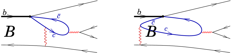
Figure 1: A diagram for a ‘generic Penguin’ process (left) where the decay along the channel $b\!\to\!c\bar{c}\,q$ produces a final state without hidden charm, simultaneously includes the ‘Intrinsic Charm’-type contribution to the same final state (right) if both ‘intrinsic’ $c$ and $\bar{c}$ annihilate with the quarks produced in the decay.

Without going into further details here, we note that an essential stumbling block in clarifying these principal elements here is lack, as of now, of a consistent OPE procedure which could be applied to such exclusive decay processes in Minkowski space. For instance, a clear separation is missing of which effects are absorbed into the decay matrix elements and which corrections are attributed to the effective weak decay Hamiltonian. Related to this, there is no clear understanding of how to integrate out the high-frequency/high-mass modes and what type of an effective Minkowskian field theory for exclusive decays would result from this. A more complex answer here may, in principle, allow for more significant strong-interaction corrections related to non-valence charm quarks, which would be absent for much heavier charm quarks.

Acknowledgments: We greatly benefited from many conversations with S. Brodsky, S. Gardner, Th. Mannel, M. Shifman, A. Vainshtein and M. Voloshin. We are grateful to S. Trine for directing our attention to paper [9], which helped us to identify an inconsistency in one of our transformation routines. N.U., I.B. and R.Z. gratefully acknowledge the hospitality of TPI, Lab. de Physique Théorique of the Université de Paris Sud and of the Institute for Theoretical Physics of the University of Zürich, respectively, where a part of this study was done. R.Z. was partly supported by the Swiss National Science Foundation and by the EU-RTN Programme, Contract No. HPEN-CT-2002-00311, “EURIDICE”. This work was supported by the NSF under grant number PHY-0355098.

Appendix

Appendix A Conventions

Gauge fields

The ordinary and covariant derivatives read

$$\partial_{\alpha}=\frac{\partial}{\partial x^{\alpha}}\,,\quad\quad D_{\alpha}=\partial_{\alpha}-it^{a}A^{a}\,,$$ (A.1)

with $t^{a}=\lambda^{a}/2$ and $\lambda^{a}$ the usual hermitian $SU(3)$ Gell-Mann matrices

$$[\lambda^{a},\lambda^{b}]=2if^{abc}\lambda^{c}\,,\quad\quad{\rm Tr}[\lambda^{a}\lambda^{b}]=2\delta^{ab}\;.$$ (A.2)

The field strength tensor and its dual are defined as

$$G_{\alpha\beta}=G_{\alpha\beta}^{a}t^{a}=i[D_{\alpha},D_{\beta}]\;,\;\tilde{G}_{\alpha\beta}=\frac{1}{2}\epsilon_{\alpha\beta\gamma\delta}G^{\gamma\delta}\;.$$ (A.3)

Electromagnetic notations

In terms of the field strength tensor the electromagnetic fields read

$$E_{i} = F_{0i}$$ (A.4)

$$B_{i} = \mbox{$\frac{1}{2}$}\epsilon_{ijk}F_{jk}\quad(F_{ij}=\epsilon_{ijk}B_{k})\quad.$$ (A.5)

The square of the field strength tensor is

$$F_{\mu\nu}F^{\mu\nu}=2(B^{2}\!-\!E^{2})\;.$$ (A.6)

Greek indices $\alpha$ run from $0$ to $3$, Latin indices $a$ run from $1$ to $3$, and the summation convention is to be understood in the following way:

$$a\cdot b=a_{\mu}b^{\mu}=a_{0}b_{0}-a_{1}b_{1}-a_{2}b_{2}-a_{3}b_{3}=a_{0}b_{0}-a_{k}b_{k}\;.$$ (A.7)

The $\epsilon$-tensor

We use the $\epsilon$-tensor convention from [11] which is the same as in Itzykson & Zuber as opposed to Bjorken & Drell,

$$\epsilon^{0123}=-\epsilon_{0123}=1\;.$$ (A.8)

Appendix B Currents in the Fock-Schwinger gauge

Here we sketch the technique used for calculating the charm currents in the external gluon field. We use the Fock-Schwinger gauge and work in momentum space. Our master equation is

$$\langle\bar{c}^{a}\Gamma c^{b}(0)\rangle_{A}=i\int\frac{d^{4}k}{(2\pi)^{4}}{\rm Tr}_{\gamma}[\Gamma\frac{1}{\hbox to0.0pt{\kern 0.55559pt/\hss}\tilde{k}\!-\!m_{c}}]_{ba}\cdot 1\;,$$ (A.9)

where $\Gamma$ is a matrix in Dirac space, $a,b$ are color indices and the ‘propagator’ must be understood as an operator:

$$(\tilde{k}_{\mu})_{ab}=k_{\mu}\delta_{ab}-\frac{i}{2}(G_{\alpha\mu})_{ab}(0)\partial_{k^{\alpha}}-\frac{1}{3}(D_{\lambda}G_{\alpha\mu})_{ab}(0)\partial_{k^{\alpha}}\partial_{k^{\lambda}}+\ldots,$$ (A.10)

with $\partial_{k_{\alpha}}=\frac{\partial}{\partial k^{\alpha}}$. We expand $1/(\hbox to0.0pt{\kern 0.55559pt/\hss}\tilde{k}-m_{c})$ in Eq. (A.9) in the gluon field strength, which yields a series in differential operators in the Fourier transform (‘momentum’) space. These act on the momentum space ‘unity’ in Eq. (A.9), which implies that the right-most derivative vanishes.

To derive this representation, we start with the definition

$$\langle\bar{c}^{a}_{\alpha}c^{b}_{\beta}(x)\rangle=\langle x|\Big{(}\frac{1}{i\hbox to0.0pt{\kern 1.88254pt/\hss}D\!-\!m_{c}}\Big{)}_{ba}^{\beta\alpha}|x\rangle$$ (A.11)

where $i\!\!\not\!\!\!{D}\!-\!m_{c}$ is the Dirac operator in the gluon background, and we have shown the spinor indices $\alpha$ and $\beta$ explicitly. We then write the coordinate matrix element $\langle x|...|x\rangle$ of the Dirac propagator in the momentum space: using  $\langle k|x\rangle=e^{ikx}$  we have (the Lorentz indices are not shown for simplicity)

$$\langle x|\frac{1}{i\hbox to0.0pt{\kern 1.88254pt/\hss}D\!-\!m_{c}}|x\rangle=\langle x|\frac{1}{i\hbox to0.0pt{\kern 0.53093pt/\hss}\partial\!+\!\hbox to0.0pt{\kern 1.65001pt/\hss}A(x)\!-\!m_{c}}|x\rangle=\sum_{p,k}\langle x|p\rangle\langle p|\frac{1}{i\hbox to0.0pt{\kern 0.53093pt/\hss}\partial\!+\!\hbox to0.0pt{\kern 1.65001pt/\hss}A(x)\!-\!m_{c}}|k\rangle\langle{k}|x\rangle =$$

$$\sum_{p,k}e^{i(p\!-\!k)x}\langle p|\frac{1}{\hbox to0.0pt{\kern 0.55211pt/\hss}k\!-\!m_{c}\!+\!\hbox to0.0pt{\kern 1.65001pt/\hss}A(i\partial_{k})}|k\rangle\,.\mbox{\hskip 85.35826pt~{}}$$ (A.12)

Since $\langle p|k\rangle=\delta(p\!-\!k)$, the latter expression upon summation over $p$ recovers the definition of the operator acting on the momentum-space unity in Eq. (A.9):

$$\sum_{p,k}\langle p|f(k;\partial_{k})|k\rangle=\sum_{p,k}f(k;\partial_{k})\delta(p\!-\!k)=\sum_{k}f(k;\partial_{k})\cdot 1\;.$$ (A.13)

The second step is to apply the Fock-Schwinger gauge $(x\!-\!x_{0})\!\cdot\!A(x)=0$, $A(x_{0})=0$. We shall set the fixed point $x_{0}$ to zero and then (for details, see Ref. ([31])

$$A_{\mu}(x)=\int_{0}^{1}d\lambda\,\lambda x^{\nu}\,G_{\nu\mu}(\lambda x)\;.$$ (A.14)

We can Taylor expand the field strength in powers of $\lambda x$ and integrate over $\lambda$. Due to the specific choice of the gauge condition the ordinary derivatives in the Taylor expansion can be replaced by the covariant derivatives, and the expansion of the gauge potential takes the following form:

$$A_{\mu}(x)=\frac{1}{2}x^{\alpha}G_{\alpha\mu}-\frac{1}{3}x^{\alpha}x^{\lambda}D_{\lambda}G_{\alpha\mu}+\ldots\;.$$ (A.15)

Using this explicit form for the gauge potential in the covariant derivative in the Dirac operator and replacing $x_{\alpha}$ by $-i\partial_{k_{\alpha}}$ we arrive at the representation Eqs. (A.9)-(A.10).

Appendix C Some elements of the 2-loop calculation $\alpha_{s}(m_{c})/m_{c}$

Here we outline the principal steps of the calculation that lead to the result in Eq. (21). The graphs are depicted in Fig 3.

Figure 2: The one-loop graph (a) and the relevant two-loop graphs (b),(c); the external gauge field lines are not shown. The two-loop graph (b) is depicted in detail in Fig. 3.

Our aim is to calculate the coefficients $C_{jk}(\mu)$ in Eq. (8). Using the universality of the OPE we can obtain those coefficients for on-shell $b$-quarks with $p=(m_{b},0,0,0)$ in the fixed gluon background, where the matrix elements are simple functions of the gluon fields.

There are six possible ways to attach a hard gluon to the one-loop graph in Fig 2a; only two contribute at order $1/m_{c}$. The gluon has to connect the $b$-quark line with the $c$ quark in the loop, Fig. 2b,c, otherwise the symmetry of the graph is the same as in the one-loop case and would bar a $1/m_{c}$ contributions.

The sum of the two-loop graphs in Figs. 2b,c reads

$$\mbox{~{}}\langle b(p)|J_{12}|b(p)\rangle=$$ (A.16)

$$\mbox{\hskip 1.99168pt~{}}-g^{2}\!\int_{kq}{\rm Tr}[\Gamma_{2}S_{c}(p\!+\!k)t^{a}\gamma^{\mu}S_{c}(q)]\,\Delta_{\mu\nu}^{ab}(k)\,\bar{b}(p)\left(t^{b}\gamma^{\nu}S_{b}(k+p)\Gamma_{1}+\Gamma_{1}S_{b}(p\!-\!k)t^{b}\gamma^{\nu}\right)b(p)$$

with $J_{12}$ defined in Eq. (9) and the trace taken over the $c$-quark spinor and color indices; the $s$-quark and gluon propagators in the external field are given below, Eqs. (A.18)-(C). We use the convention $\int_{y}=\int d^{d}y$ and $\int_{k}=\int\frac{d^{d}k}{(2\pi)^{d}}$. In the heavy quark limit the $b$-quark propagator $S_{b}$ reduces to

$$S_{b}(p\pm k)=\frac{\hbox to0.0pt{\kern 0.50314pt/\hss}p\pm\hbox to0.0pt{\kern 0.55211pt/\hss}k+m_{b}}{(p\pm k)^{2}-m_{b}^{2}+i0}\stackrel{{\scriptstyle m_{b}\!\to\infty}}{{\longrightarrow}}\frac{1}{\pm k_{0}+i0}=\pm\,P\frac{1}{k_{0}}-i\pi\delta(k_{0})\;.$$ (A.17)

Figure 3: The graphs corresponding to Fig. 2b which contribute to order $\alpha_{s}(m_{c})/m_{c}$ in the fixed-point gauge. The double line shows the static $b$ quark and the loop stands for charm quark. The two external gluon lines generically represent the operators in Eqs. (20), as it comes out naturally in this gauge.

Only the $\nu\!=\!0$ vertex survives the static limit, and the expression becomes

$$\langle b(p)|J_{12}|b(p)\rangle=\int_{kq}{\rm Tr}[\Gamma_{2}S_{c}(k+q)t^{a}\gamma^{\mu}S_{c}(q)]\,\Delta^{ab}_{\mu 0}(k)\;\bar{b}\left(i\pi\delta(k_{0})\{t^{b}\!,\Gamma_{1}\}-P\mbox{{\large$\frac{1}{k_{0}}$}}\,[t^{b}\!,\Gamma_{1}]\right)b$$

It can be shown that the contribution of the principal value piece $P\frac{1}{k_{0}}$ vanishes upon integration; we have explicitly verified this in our calculation.

As the next step we need to put the appropriate propagators in the external field and to project out the operators in Eq. (20). As discussed in the previous Appendix, **for external gluon fields we use the background field method in the Fock-Schwinger gauge $x\!\cdot\!A(x)\!=\!0$ where the gauge potential is expanded directly in the gauge invariant field strength; c.f. Ref [31] for a pedagogical introduction. For internal gluon fields a different gauge may be used; we adopt the Feynman gauge for it.

The gluonic operator parts in Eq. (20) carry dimension four and may either come from a single propagator, or from two separate propagators each contributing one gluonic field strength of mass dimension two. It is most economic to choose the fixed point to be the position of the local four-quark operator. With this choice the $b$-quark propagator does not interact with soft gluons because the Wilson line is unity in this gauge; other soft contributions to the $b$ quark propagator vanish in the heavy quark limit. There remain six graphs shown in Fig. 3 out of ten possible combinatorial possibilities for Fig. 2b, plus similar diagrams corresponding to Fig. 2c. They will be examined below.

Propagators in the external field

The massless fermion propagator in the external field was given in Ref. [31], Eqs. (2.30)-(2.31); the gauge potential propagator in the external field was also presented in [31] for the case where one of the endpoints is the fixed point, Eq. (2.35). For the fermion propagator we need to include mass. The diagrams in Fig. 3 also include gluon Green function between two general points. Both generalizations are not difficult.

We arrange the propagators in increasing dimension of the external gluon fields:

$$\Delta_{\mu\nu}^{ab}(x,y)\mbox{~{}} = \mbox{~{}}-i\,\langle TA_{\mu}^{a}(x)A_{\nu}^{b}(y)\rangle=\Delta^{(0)ab}_{\mu\nu}(x,y)+\Delta^{(2)ab}_{\mu\nu}(x,y)+\Delta^{(3)ab}_{\mu\nu}(x,y)+\Delta^{(4)ab}_{\mu\nu}(x,y)$$

$$S(x,y)\mbox{~{}} = \mbox{~{}}-i\,\langle T\psi(x)\bar{\psi}(y)\rangle_{A}=S^{(0)}(x,y)+S^{(2)}(x,y)+S^{(3)}(x,y)+S^{(4)}(x,y)\;,$$ (A.18)

The propagators are obtained using the background field Lagrangian. With the fixed point $x_{0}\!=\!0$ the used terms for the fermion propagator are

$$S^{(0)}(x,y)\mbox{~{}} \equiv \mbox{~{}}S(x\!-\!y)=\int_{p}e^{-ip\!\cdot\!(x\!-\!y)}S(p)\equiv\int_{p}\,e^{-ip\!\cdot\!(x\!-\!y)}\frac{\hbox to0.0pt{\kern 0.50314pt/\hss}p+m}{p^{2}\!-\!m^{2}}\;,$$ (A.19)

$$S^{(2)}(x,y)\mbox{~{}} = \mbox{~{}}-\frac{1}{2}G_{\alpha\beta}(0)\left\{\begin{array}[]{l}(i\partial_{p}+x)_{\alpha}\\ (-i\partial_{q}+y)_{\alpha}\end{array}\right\}\int_{p}e^{-ip\cdot(x\!-\!y)}S(p)\gamma_{\beta}S(q)\;,$$ (A.22)

$$S^{(4)}(x,y)\mbox{~{}} = \mbox{~{}}\frac{1}{4}G_{\alpha\beta}G_{\gamma\delta}\left\{\begin{array}[]{l}(-i\partial_{p}\!-\!x)_{\alpha}(-i\partial_{p+q}\!-\!x)_{\gamma}\\ (-i\partial_{q+k}+y)_{\alpha}(-i\partial_{k}+y)_{\gamma}\end{array}\right\}\int_{p}e^{-ip\cdot(x\!-\!y)}S(p)\gamma_{\beta}S(q)\gamma_{\delta}S(k)$$ (A.24)

$$- \mbox{~{}}\frac{1}{8}\nabla_{\alpha}\nabla_{\beta}G_{\gamma\delta}\left\{\begin{array}[]{l}(i\partial_{p}+x)_{\alpha}(i\partial_{p}+x)_{\beta}(i\partial_{p}+x)_{\gamma}\\ (y\!-\!i\partial_{q})_{\alpha}(y\!-\!i\partial_{q})_{\beta}(y\!-\!i\partial_{q})_{\gamma}\end{array}\right\}\int_{p}e^{-ip\cdot(x\!-\!y)}S(p)\gamma_{\delta}S(q)\;,$$ (A.26)

and for gluons

$$\Delta_{\mu\nu}^{\!(0)\,ab}(x,y)\mbox{~{}} = \mbox{~{}}g_{\mu\nu\,}\delta^{ab}\int_{p}e^{-ip\!\cdot\!(x\!-\!y)}\frac{-1}{p^{2}}\;,$$ (A.27)

$$\Delta_{\mu\nu}^{(2)ab}(x,y)\mbox{~{}} = \mbox{~{}}-2G_{\mu\nu}^{ab}(0)\int_{p}\,e^{-ip\!\cdot\!(x\!-\!y)}\frac{1}{p^{4}}\;,$$

$$+ \mbox{~{}}ig_{\mu\nu}G_{\alpha\beta}^{ab}(-i\partial_{k}+y)_{\alpha}\int_{p}e^{-ip\cdot(x\!-\!y)}\frac{p_{\beta}}{p^{2}}\frac{1}{k^{2}}\;,$$

$$\Delta_{\mu\nu}^{(4)ab}(x,y)\mbox{~{}} = \mbox{~{}}-4G_{\mu\lambda}^{ac}G_{\lambda\nu}^{cb}\int_{p}e^{-ip\cdot(x\!-\!y)}\frac{1}{p^{6}}$$

$$- \mbox{~{}}\nabla_{\alpha}\nabla_{\beta}G_{\mu\nu}^{ab}(y\!-\!i\partial_{k})_{\alpha}(y\!-\!i\partial_{k})_{\beta}\int_{p}e^{-ip\cdot(x\!-\!y)}\frac{1}{p^{2}}\frac{1}{k^{2}}$$

$$- \mbox{~{}}\frac{1}{4}g_{\mu\nu}G^{ac}_{\alpha\lambda}G^{cb}_{\lambda\delta}(y\!-\!i\partial_{k})_{\alpha}(y\!-\!i\partial_{k})_{\delta}\int_{p}e^{-ip\cdot(x\!-\!y)}\frac{1}{p^{2}}\frac{1}{k^{2}}$$

$$+ \mbox{~{}}\frac{i}{4}g_{\mu\nu}(\nabla_{\alpha}\nabla_{\beta}G_{\gamma\delta})^{ab}(y\!-\!i\partial_{k})_{\alpha}(y\!-\!i\partial_{k})_{\beta}(y\!-\!i\partial_{k})_{\gamma}\int_{p}e^{-ip\cdot(x\!-\!y)}\frac{p_{\delta}}{p^{2}}\frac{1}{k^{2}}\,.$$

For the fermion propagators we gave different possible representations which can be chosen pursuant to calculational convenience, see below. The momenta $q$ and $k$ must be set equal to $p$ after taking derivatives. For the gluon fields the matrix notation $G^{ac}_{\mu\nu}\!=\!f^{abc}G^{b}_{\mu\nu}$ is assumed. In fact, one can do without a coordinate representation if one of the endpoints of the propagator coincides with the fixed point. This is the case for the $c$ quark lines, but not for the gluon propagator in Fig. 3. $S^{(3)}$ or $\Delta^{(3)}$, respectively, do not contribute, and we do not give $S^{(4)}$ and $\Delta^{(4)}$ for brevity.

After putting in the propagators and evaluating the traces the needed integral takes the generic form

$$I_{nm}(\alpha,\beta,\gamma)=\int_{kq}\delta(k_{0})\frac{k_{\mu_{1}}\dots k_{\mu_{n}}q_{\nu_{1}}\dots q_{\nu_{m}}}{(k^{2})^{\alpha}(q^{2}\!-\!m^{2})^{\beta}((k+q)^{2}\!-\!m^{2})^{\gamma}}\>,\qquad 0\!\leq\!m+n\!\leq\!6\;.$$ (A.28)

Those integrals are in fact easily calculated in arbitrary dimensions $d$. Rewriting the propagators as $(q^{2}\!-\!m^{2})^{a}=(-1)^{a}(\vec{q}^{\,2}\!+\!(m^{2}\!-\!q_{0}^{2}))^{a}$ suggests integrating over ${\rm d}^{d\!-\!1}q$ and ${\rm d}^{d\!-\!1}k$  first. We combine the denominators by introducing a Feynman-Schwinger parameter which is integrated over at the end yielding the Euler Beta-function. The variable $k_{0}$ is fixed by the $\delta$-function and the remaining integration over $q_{0}$ is elementary.

For the first step the following master integral is needed:

$$\mbox{~{}}J(a,b,c;d)=\int\frac{{\rm d}^{d}k}{(2\pi)^{d}}\,\frac{{\rm d}^{d}q}{(2\pi)^{d}}\>\frac{1}{(k^{2})^{a}(q^{2}\!+\!m^{2})^{b}((k\!+\!q)^{2}\!+\!m^{2})^{c}}\,=$$

$$\mbox{\hskip 14.22636pt~{}}\frac{1}{(4\pi)^{d}}\,\frac{\Gamma(\mbox{$\frac{d}{2}$}\!-\!a)\Gamma(a\!+\!b\!+\!c\!-\!d)}{\Gamma(b)\Gamma(c)\Gamma(\mbox{{\small$\frac{d}{2}$}})}\,B(a\!+\!b\!-\!\mbox{$\frac{d}{2}$},a\!+\!c\!-\!\mbox{$\frac{d}{2}$})\>(m^{2})^{d\!-\!(a\!+\!b\!+\!c)}$$ (A.29)

and, therefore the scalar integral in Eq. (A.28) is

$$\mbox{~{}}I_{00}(a,b,c;d\!+\!1)=\int\frac{{\rm d}^{d}k}{(2\pi)^{d}}\,\frac{{\rm d}^{d}q}{(2\pi)^{d}}\,\frac{{\rm d}q_{0}}{2\pi}\>\frac{(-1)^{a+b+c}}{(k^{2})^{a}(q^{2}\!+\!(m^{2}-q_{0}^{2}))^{b}((k\!+\!q)^{2}+(m^{2}-q_{0}^{2}))^{c}}\,=$$

$$\mbox{\hskip 5.69054pt~{}}\frac{i(-1)^{a+b+c}}{(4\pi)^{d+\mbox{{\footnotesize$\frac{1}{2}$}}}}\,\frac{\Gamma(\mbox{$\frac{d}{2}$}\!-\!a)\Gamma(a\!+\!b\!+\!c\!-\!d\!-\!\mbox{{\small$\frac{1}{2}$}})}{\Gamma(b)\Gamma(c)\Gamma(\mbox{$\frac{d}{2}$})}\,B(a\!+\!b\!-\!\mbox{$\frac{d}{2}$},a\!+\!c\!-\!\mbox{$\frac{d}{2}$})\>(m^{2})^{d\!-\!(a\!+\!b\!+\!c)\!+\!\mbox{{\footnotesize$\frac{1}{2}$}}}.$$ (A.30)

In view of proliferating combinatorial possibilities we implemented the evaluation of the tensor integrals algorithmically starting from the scalar master integral Eq. (A.30).

The $c$-quark loop potentially has UV divergences and the gluon loop potentially has IR divergences. Since the one-loop contribution to this order in $1/m_{c}$ vanishes, the divergences must disappear in the sum over all the graphs. The only diagrams involving IR or UV divergent integrals are those from Figs. 3 d,e,f which are those where a gluon is emitted from the hard gluon line. Explicit calculations yield that, in fact, the divergences cancel in each individual graph.

Furthermore, a Furry-type analysis of the symmetries of the graphs can be done. Since the Gell-Mann matrices have no definite transformation properties under transposition, one has to resort to Hermitian conjugation. This distinguishes the QCD analysis from the QED case. The outcome is that the two graphs in Fig. 3d,e are equal; the two graphs in Fig. 3a,b are equal in the vector channel, but not in the axial channel. This is verified explicitly in the calculations. Another nontrivial consistency check would be to introduce a generic Fock-Schwinger fixed point and to observe its disappearance from the final result. This would require, however more involved calculations and the evaluation of four more graphs.

References

• [1] I. Bigi, N. Uraltsev and A. Vainshtein, Phys. Lett. B293 (1992) 430.
• [2] B. Blok and M. Shifman, Nucl. Phys. B399 (1993) 441 and 459.
• [3] M.A. Shifman, A.I. Vainshtein and V.I. Zakharov, Nucl. Phys.  B147 385 (1979);
V.A. Novikov, M.A. Shifman, A.I. Vainshtein and V.I. Zakharov, Nucl. Phys.  B249 445 (1985).
• [4] M. Voloshin and M. Shifman, Yad. Fiz.  41 (1985) 187 [Sov. J. Nucl. Phys.  41 (1985) 120].
• [5] I. Bigi and N. Uraltsev, Nucl. Phys.  B423 (1994) 33.
• [6] K. Melnikov and A. Yelkhovsky, Phys. Rev.  D 59 (1999) 114009;
A. Hoang, Phys. Rev.  D 61 (2000) 034005;
M. Beneke and A. Signer, Phys. Lett.  B 471 (1999) 233.
• [7] O. Buchmueller and H. Flaecher, Phys. Rev. D73 (2006) 073008.
• [8] D. Benson, I. Bigi, Th. Mannel and N. Uraltsev, Nucl. Phys. B665 (2003) 367.
• [9] J.-M. Gerard, C. Smith and S. Trine, Nucl. Phys. B730 (2005) 1.
• [10] R. Zwicky, IPPP-05-72, DCPT-05-144 (in preparation).
• [11] M. Franz, M.V. Polyakov and K. Goeke, Phys.  Rev.  D62 (2000) 074024.
• [12] I. Bigi, M. Shifman and N.G. Uraltsev, Ann. Rev. Nucl. Part. Sci. 47 (1997) 591.
• [13] N. Uraltsev, Phys. Lett. B585 (2004) 253; ibid. B545 (2002) 337.
• [14] R. Lebed and N. Uraltsev, Phys. Rev. D62 (2000) 094011.
• [15] G. ’t Hooft, Nucl. Phys.  B75 (1974) 461.
• [16] N. Uraltsev, hep-ph/0409125; in Proc. of the Continuous Advances in QCD 2004, ed. T. Gherghetta, World Scientific, Singapore (2004), p.100.
• [17] M. Shifman and A. Vainshtein, Phys. Rev.  D71 (2005) 074010.
• [18] I.I. Bigi, M. Shifman, N.G. Uraltsev and A. Vainshtein, Phys. Rev. D52 (1995) 196.
• [19] D. Pirjol and N. Uraltsev, Phys. Rev. D59 (1999) 034012.
• [20] A. Chodos et al., Phys. Rev.  D9 (1974) 3471.
• [21] B. Chibisov, R. Dikeman, M. Shifman, N.G. Uraltsev, Int. Journ. Mod. Phys.  A12 (1997) 2075.
• [22] M. Shifman, in: Boris Ioffe Festschrift “At the Frontier of Particle Physics/Handbook of QCD”, M. Shifman Ed.), World Scientific, Singapore, 2001.
• [23] N. Uraltsev, Int. Journ. Mod. Phys. A14 (1999) 4641.
• [24] B. Blok, L. Koyrakh, M. Shifman and A. Vainshtein, Phys. Rev. D49 (1994) 3356.
• [25] P. Gambino and N. Uraltsev, Eur. Phys. J. C34 (2004) 181.
• [26] N.  Uraltsev, Int. J. Mod. Phys. A 20 (2005) 2099.
• [27] V. Aquila, P. Gambino, G. Ridolfi and N. Uraltsev, Nucl. Phys. B719 (2005) 77.
• [28] S.J. Brodsky and S. Gardner, Phys. Rev.  D65 (2002) 054016.
• [29] A. I. Vainshtein, V. I. Zakharov and M. A. Shifman, JETP Lett.  22 (1975) 55 [Pisma Zh. Eksp. Teor.  Fiz.  22 (1975) 123];
M. A. Shifman, A. I. Vainshtein and V. I. Zakharov, Nucl.  Phys.  B 120 (1977) 316.
• [30] I. Bigi and N. Uraltsev, Phys. Lett.  B280 (1992) 271.
• [31] V. A. Novikov, M. A. Shifman, A. I. Vainshtein and V. I. Zakharov, Fortsch. Phys.  32 (1985) 585.