XIth International Conference on
Elastic and Diffractive Scattering
Château de Blois, France, May 15 - 20, 2005

THE HEIDELBERG POMERON

One of the challenges in quantum chromodynamics (QCD) is the description and understanding of hadronic high-energy scattering. Since the momentum transfers can be small, the QCD coupling constant is too large for a reliable perturbative treatment. Non-perturbative QCD is needed which is rigorously only available as a computer simulation on Euclidean lattices.

An interesting phenomenon observed in hadronic high-energy scattering is the rise of the total cross sections with increasing c.m. energy. While the rise is slow in hadronic reactions of large particles such as protons, pions, kaons, or real photons, it is steep if only one small particle is involved such as an incoming virtual photon or an outgoing charmonium.

In this work, we develop a model combining perturbative and non-perturbative QCD to compute high-energy reactions of hadrons and photons with special emphasis on saturation effects that manifest the $S$-matrix unitarity. Aiming at a unified description of hadron-hadron, photon-hadron, and photon-photon reactions involving real and virtual photons as well, we follow the functional integral approach to high-energy scattering in the eikonal approximation, in which the $S$-matrix element factorizes into the universal correlation of two light-like Wegner-Wilson loops $S_{DD}$ and reaction-specific light-cone wave functions. The light-like Wegner-Wilson loops describe color-dipoles given by the quark and antiquark in the meson or photon and in a simplified picture by a quark and diquark in the baryon. Consequently, hadrons and photons are described as color-dipoles with size and orientation determined by appropriate light-cone wave functions. Thus, the loop-loop correlation function $S_{DD}$ is the basis for our unified description. We compute the $T$-matrix in a functional integral approach developed for parton-parton scattering in the eikonal approximation. In this approach, the $T$-matrix element for the reaction $ab\rightarrow cd$ factorizes as follows

$$T_{ab\rightarrow cd}(s,t)=2is\int\!\!d^{2}b_{\!\perp}e^{i{\vec{q}}_{\!\perp}{\vec{b}}_{\!\perp}}\int\!\!dz_{1}d^{2}r_{1}\!\int\!\!dz_{2}d^{2}r_{2}$$

$$\times\psi_{c}^{*}(z_{1},{\vec{r}}_{1})\,\psi_{d}^{*}(z_{2},{\vec{r}}_{2})\left[1-S_{DD}({\vec{b}}_{\!\perp},z_{1},{\vec{r}}_{1},z_{2},{\vec{r}}_{2})\right]\psi_{a}(z_{1},{\vec{r}}_{1})\,\psi_{b}(z_{2},{\vec{r}}_{2})\ ,$$ (1)

where the loop-loop correlation function

$$S_{DD}({\vec{b}}_{\!\perp},z_{1},{\vec{r}}_{1},z_{2},{\vec{r}}_{2})=\Big{\langle}W[C_{1}]W[C_{2}]\Big{\rangle}_{G}$$ (2)

describes the elastic scattering of two color-dipoles (DD) with transverse size and orientation ${\vec{r}}_{i}$ and longitudinal quark momentum fraction $z_{i}$ at impact parameter ${\vec{b}}_{\!\perp}$, transverse momentum transfer ${\vec{q}}_{\!\perp}$ ($t=-{\vec{q}}_{\!\perp}^{\,\,2}$) and c.m. energy squared $s$.

The path of each color-dipole is represented by a light-like QCD Wegner-Wilson loop

$$W[C_{1,2}]=\frac{1}{N_{c}}\mbox{Tr}\,{\cal P}\exp\!\left[-ig\!\oint_{\scriptsize C_{1,2}}\!\!dz^{\mu}{\cal G}_{\mu}(z)\right]\ ,$$ (3)

where $N_{c}$ is the number of colors, Tr the trace in color space, $g$ the strong coupling, and ${\cal G}_{\mu}(z)={\cal G}_{\mu}^{a}(z)t^{a}$ the gluon field with the $SU(N_{c})$ group generators $t^{a}$ that demand the path ordering indicated by ${\cal P}$. Quark-antiquark dipoles are represented by loops in the fundamental $SU(N_{c}=3)$ representation. In the eikonal approximation to high-energy scattering the $q$ and ${\bar{q}}$ paths form straight light-like trajectories. Figure 1 illustrates the space-time (a) and transversal (b) arrangement of these loops.

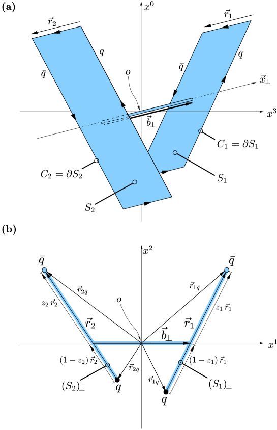
Figure 1: Space-time (a) and transverse (b) arrangement of the Wegner-Wilson loops.

The QCD vacuum expectation value $\langle\ldots\rangle_{G}$ in the loop-loop correlation function represents functional integrals. To compute the loop-loop correlation function, we transform the line integrals over the loops $C_{1,2}$ into integrals over surfaces $S_{1,2}$ with $\partial S_{1,2}=C_{1,2}$ by applying the non-Abelian Stokes’ theorem and the cumulant expansion truncated at $n=2$ Consequently, all higher cumulants, $K_{n}$ with $n>2$, vanish and the loop-loop correlation function can be expressed in terms of $K_{2}$

$$\!\!\!\!\!\!\!\!\!\!\!\Big{\langle}W[C_{1}]W[C_{2}]\Big{\rangle}_{G}$$

$$\!\!\!\!\!\!\!\!\!\!\!=\frac{1}{N_{c}^{2}}\mbox{Tr}_{2}\exp\!\left[-\frac{g^{2}}{8}\!\int_{S}\!d\sigma^{\mu\nu}(x_{1})\!\int_{S}\!d\sigma^{\rho\sigma}(x_{2})\Big{\langle}{\cal P}_{S}\,\hat{\cal{G}}_{\mu\nu}(o,x_{1};C_{x_{1}o})\hat{\cal{G}}_{\rho\sigma}(o,x_{2};C_{x_{2}o})\Big{\rangle}_{G}\right].$$

(4)

Due to the color-neutrality of the vacuum, the gauge-invariant bilocal gluon field strength correlator simplifies

$$\Big{\langle}\frac{g^{2}}{4\pi^{2}}\,{\cal G}^{a}_{\mu\nu}(o,x_{1};C_{x_{1}o}){\cal G}^{b}_{\rho\sigma}(o,x_{2};C_{x_{2}o})\Big{\rangle}_{G}=:\frac{1}{4}\delta^{ab}F_{\mu\nu\rho\sigma}(x_{1},x_{2},o;C_{x_{1}o},C_{x_{2}o})\ .$$ (5)

The quantity $F_{\mu\nu\rho\sigma}$ is obtained from the stochastic vacuum model. We define

$$\chi_{S_{i}S_{j}}:=-\,i\frac{\pi^{2}}{4}\int_{S_{i}}\!d\sigma^{\mu\nu}(x_{1})\int_{S_{j}}\!d\sigma^{\rho\sigma}(x_{2})F_{\mu\nu\rho\sigma}(x_{1},x_{2},o;C_{x_{1}o},C_{x_{2}o})\ ,$$ (6)

then

$$\Big{\langle}W[C_{1}]W[C_{2}]\Big{\rangle}_{G} = \frac{1}{N_{c}^{2}}\mbox{Tr}_{2}\exp\!\Bigg{[}-i\,\frac{1}{2}\Big{\{}\,\left(\chi_{S_{1}S_{2}}+\chi_{S_{2}S_{1}}\right)\big{(}t^{a}\,\otimes\,t^{a}\big{)}$$ (7)

$$+\,\chi_{S_{1}S_{1}}\big{(}t^{a}t^{a}\,\otimes\,{1\!\rm l}\big{)}+\chi_{S_{2}S_{2}}\big{(}{1\!\rm l}\,\otimes\,t^{a}t^{a}\big{)}\,\Big{\}}\,\Bigg{]}\ .$$

Our ansatz for the tensor structure of $F_{\mu\nu\rho\sigma}$ leads to $\chi_{S_{1}S_{1}}=\chi_{S_{2}S_{2}}=0$ for light-like loops, and also to $\chi_{S_{1}S_{2}}=\chi_{S_{2}S_{1}}=:\chi$. For the evaluation of the trace of the remaining exponential, we project on the $\bar{3}$ and $6$ representations and obtain:

$$\Big{\langle}W[C_{1}]W[C_{2}]\Big{\rangle}_{G}=\frac{2}{3}\exp\!\left[-\frac{i}{3}\chi\right]+\frac{1}{3}\exp\!\left[\frac{2i}{3}\chi\right]\$$ (8)

We decompose the gauge-invariant bilocal gluon field strength correlator (5) into a perturbative ($P$) and non-perturbative ($N\!P$) component

$$F_{\mu\nu\rho\sigma}=F_{\mu\nu\rho\sigma}^{N\!P}+F_{\mu\nu\rho\sigma}^{P}\ .$$ (9)

Here, $F_{\mu\nu\rho\sigma}^{N\!P}$ gives the low frequency background field contribution modelled by the non-perturbative stochastic vacuum model (SVM) and $F_{\mu\nu\rho\sigma}^{P}$ the additional high frequency contributions described by perturbative gluon exchange. Such a decomposition is supported by lattice QCD computations of the Euclidean field strength correlator. Note that $\chi=\chi_{c}^{N\!P}+\chi_{nc}^{N\!P}+\chi^{P}$ is a real-valued function. Since, in addition, the wave functions $|\psi_{i}(z_{i},\vec{r}_{i})|^{2}$ used in this work are invariant under the replacement $(\vec{r}_{i}\rightarrow-\vec{r}_{i},z_{i}\rightarrow 1-z_{i})$, the $T$-matrix element becomes purely imaginary and reads for $N_{c}=3$ (for details we refer to the literature [3,4,5,6,7])

$$\!\!\!\!\!\!\!\!\!\!\!\!\!T(s,t) = 2is\int\!\!d^{2}b_{\!\perp}e^{i{\vec{q}}_{\!\perp}{\vec{b}}_{\!\perp}}\int\!\!dz_{1}d^{2}r_{1}\!\int\!\!dz_{2}d^{2}r_{2}\,\,|\psi_{1}(z_{1},\vec{r}_{1})|^{2}\,\,|\psi_{2}(z_{2},\vec{r}_{2})|^{2}$$ (10)

$$\!\!\!\!\!\!\!\!\!\!\times\left[1-\frac{2}{3}\cos\!\left(\frac{1}{3}\chi({\vec{b}}_{\!\perp},z_{1},\vec{r}_{1},z_{2},\vec{r}_{2})\!\right)-\frac{1}{3}\cos\!\left(\frac{2}{3}\chi({\vec{b}}_{\!\perp},z_{1},\vec{r}_{1},z_{2},\vec{r}_{2})\!\right)\right].$$

The good agreement of the computed total cross sections with the experimental data is shown in Fig. 2. Here, the solid lines represent the theoretical results for $pp$, $\pi^{+}p$, $K^{+}p$, $\gamma p$, and $\gamma\gamma$ scattering and the dashed lines the ones for $p{\bar{p}}$, $\pi^{-}p$, and $K^{-}p$ scattering. The $pp$, $p{\bar{p}}$, $\pi^{\pm}p$, $K^{\pm}p$, $\gamma p$ and $\gamma\gamma$ data taken at accelerators are indicated by the closed circles while the closed squares (Fly’s eye data) and the open circles (Akeno data) indicate cosmic ray data. Concerning the photon-induced reactions, only real photons are considered.

The prediction for the total $pp$ cross section at LHC ($\sqrt{s}=14\,\mbox{TeV}$) is $\sigma^{tot}_{pp}=114.2\,\mbox{mb}$ in good agreement with the cosmic ray data. Compared with other works, our LHC prediction is close to the one of Block et al., $\sigma^{tot}_{pp}=108\pm 3.4\,\mbox{mb}$, but considerably larger than the one of Donnachie and Landshoff, $\sigma^{tot}_{pp}=101.5\,\mbox{mb}$.

The differences between $ab$ and $\bar{a}b$ reactions for $\sqrt{s}\lesssim 100\,\mbox{GeV}$ result solely from the different reggeon contributions which die out rapidly as the energy increases. The pomeron contribution to $ab$ and $\bar{a}b$ reactions is, in contrast, identical and increases as the energy increases. It thus governs the total cross sections for $\sqrt{s}\gtrsim 100\,\mbox{GeV}$ where the results for $ab$ and $\bar{a}b$ reactions coincide.

The differences between $pp$ ($p{\bar{p}}$), $\pi^{\pm}p$, and $K^{\pm}p$ scattering result from the different transverse extension parameters, $S_{p}=0.86\,\mbox{fm}>S_{\pi}=0.607\,\mbox{fm}>S_{K}=0.55\,\mbox{fm}$. Since a smaller transverse extension parameter favors smaller dipoles, the total cross section becomes smaller, and the short distance physics described by the perturbative component becomes more important and leads to a stronger energy growth due to $\epsilon^{P}=0.73>\epsilon^{N\!P}=0.125$. In fact, the ratios $\sigma^{tot}_{pp}/\sigma^{tot}_{\pi p}$ and $\sigma^{tot}_{pp}/\sigma^{tot}_{Kp}$ converge slowly towards unity with increasing energy as can already be seen in Fig. 2. For real photons, the transverse size is governed by the constituent quark masses $m_{f}(Q^{2}=0)$, where the light quarks have the strongest effect, i.e. $\sigma^{tot}_{\gamma p}\propto 1/m_{u,d}^{2}$ and $\sigma^{tot}_{\gamma\gamma}\propto 1/m_{u,d}^{4}$. Furthermore, in comparison with hadron-hadron scattering, there is the additional suppression factor of $\alpha$ for $\gamma p$ and $\alpha^{2}$ for $\gamma\gamma$ scattering coming from the photon-dipole transition. In the $\gamma\gamma$ reaction, also the box diagram contributes but is neglected since its contribution to the total cross section is less than 1%.

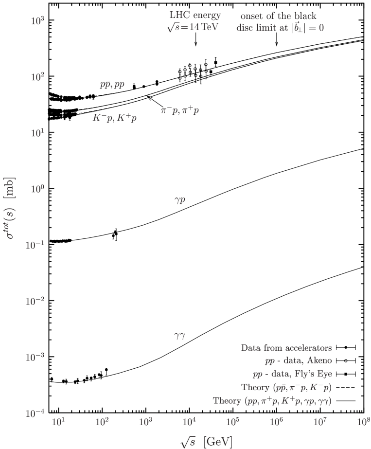
Figure 2: The total cross section $\sigma^{tot}$ is shown as a function of the c.m. energy $\sqrt{s}$ for $pp$, $p{\bar{p}}$, $\pi^{\pm}p$, $K^{\pm}p$, $\gamma p$ and $\gamma\gamma$ scattering. The solid lines represent the model results for $pp$, $\pi^{+}p$, $K^{+}p$, $\gamma p$ and $\gamma\gamma$ scattering and the dashed lines the ones for $p{\bar{p}}$, $\pi^{-}p$, and $K^{-}p$ scattering. The $pp$, $p{\bar{p}}$, $\pi^{\pm}p$, $K^{\pm}p$, $\gamma p$ and $\gamma\gamma$ data taken at accelerators are indicated by the closed circles while the closed squares (Fly’s eye data) and the open circles (Akeno data) indicate cosmic ray data. The arrows at the top point to the LHC energy, $\sqrt{s}=14\,\mbox{TeV}$, and to the onset of the black disc limit in $pp$ ($p{\bar{p}}$) reactions, $\sqrt{s}\approx 10^{6}\,\mbox{GeV}$.

To conclude we give a list of references to the work done in our group on high-energy scattering during the last years: Ref. [1] derives the Hamiltonian for a $q\bar{q}$-state on the light cone from the calculation of a single Wegner-Wilson loop near the light cone. A consistent derivation of the wave functions and the scattering is very important. Ref. [2] presents arguments for geometrical scaling and calculations that the energy dependence of high-energy scattering is related to critical correlations [6,8] of Wilson lines approaching the light cone in an effective $2+1$-dimensional QCD which is simulated in Ref. [9] on the lattice. Refs. [3,10] calculate from the stochastic vacuum model the constant and $\log(1/x)$ term in the gluon distribution, which are used in Ref. [3] as input to a DGLAP-calculation of the proton structure function. Refs. [4,5,7,12] contain calculations closely related to the subject of this talk. Ref. [4] relates the loop-loop correlation in Euclidean space to the loop-loop correlation in Minkowski space. Ref. [5] describes how the nonperturbative string can be decomposed into many perturbative dipoles which allow to calculate the unintegrated gluon distribution. Ref. [7] explains the contents of this talk in great detail, it also contains further references to other work left out in this talk. Ref. [12] discusses the specific behavior of the dipole-proton cross section for large dipoles in the stochastic vacuum model and calculates vector-meson resonance production cross sections. Resonances have larger sizes than groundstate hadrons and are therefore sensitive to the cross section for large dipoles. Ref. [11] makes the case for a soft and hard Pomeron picture of the proton structure function using the stochastic model for the soft pomeron and perturbation theory for the hard pomeron.

This work owes a great deal to my colleagues H.G. Dosch and O. Nachtmann in Heidelberg who have developed the basics of the loop-loop correlation model and with whom I have had the pleasure to collaborate.

References

References

[1]
H.J. Pirner and N. Nurpeissov,
Phys. Lett. B 595, 379 (2004).
[2]
H.J. Pirner,
Acta Phys. Polon. B 35, 265 (2004).
Contributed to Light-Cone Workshop: Hadrons and Beyond
(LC 03), Durham, England, 5-9 Aug 2003.
[3]
H.J. Pirner, A.I. Shoshi and G. Soyez,
Eur. Phys. J. C 33, 63 (2004).
[4]
A.I. Shoshi, F.D. Steffen, H.G. Dosch and H.J. Pirner,
Phys. Rev. D 68, 074004 (2003).
[5]
A.I. Shoshi, F.D. Steffen, H.G. Dosch and H.J. Pirner,
Phys. Rev. D 66, 094019 (2002).
[6]
H.J. Pirner and F. Yuan
Phys. Rev. D 66, 034020 (2002).
[7]
A.I. Shoshi, F.D. Steffen and H.J. Pirner,
Nucl. Phys. A 709, 131 (2002).
[8]
H.J. Pirner,
Phys. Lett. B 521, 279 (2001).
[9]
E.M. Ilgenfritz, Y.P. Ivanov and H.J. Pirner,
Phys. Rev. D 62, 054006 (2000).
[10] H.G. Dosch, A. Hebecker, A. Metz and H.J. Pirner, Nucl. Phys. B 568, 287 (2000).
[11] U. D’Alesio, A. Metz, and H.J. Pirner, Eur. Phys. J. C 9, 601 (1999).
[12] G. Kulzinger, H.G. Dosch and H.J. Pirner, Eur. Phys. J. C 7, 73 (1999).