Black Holes at Accelerators

Abstract

In theories with large extra dimensions and TeV-scale gravity, black holes are copiously produced in particle collisions at energies well above the Planck scale. I briefly review some recent work on the phenomenology of this process, with emphasis on theoretical uncertainties and possible strategies for measuring the number of extra dimensions.

I INTRODUCTION

One of the most surprising and exciting possibilities for new physics at future colliders is the production of microscopic black holes Giddings:2001bu ; Dimopoulos:2001hw , which can occur in theories with large extra dimensions Antoniadis:1990ew . String theory suggests a scenario in which the Standard Model particles are confined to a submanifold with the familiar three spatial dimensions (the ‘brane’), while gravity is free to propagate in the full $(3+n)$-dimensional space (the ‘bulk’). In that case the fundamental $(4+n)$-dimensional Planck scale could be much lower than its effective 4-dimensional value, possibly of the order of TeV. Then gravity would look weak on distance scales large compared to the size of the extra dimensions, but could become as strong as the other forces at short distances. Parton-parton collisions with centre-of-mass energies well above this scale could be treated as $(4+n)$-dimensional classical gravitational interactions. Numerical studies suggest that in such circumstances the probability of coalescence to form a microscopic black hole would be large Yoshino:2002tx ; Yoshino:2005hi . The black hole would be a powerful source of Hawking radiation, decaying rapidly into all kinds of Standard Model particles. From a study of the decay products, it might be possible to deduce the number and size of the extra dimensions.

In this paper I shall review some recent work on the above scenario. We shall see that, even if one accepts the basic assumption of TeV-scale gravity in extra dimensions, there are many uncertainties and gaps in our understanding, which make reliable predictions impossible at present. Nevertheless one can build models and simulations that allow one to explore different options for filling in the gaps, and enable experimentalists to start thinking about how they might analyse black hole events.

I apologise for not mentioning all relevant topics and papers in this short review. For more complete discussion and references, please see Harris:2004xt and Chris Harris’s thesis Harris:2004mf .

II BLACK HOLE PRODUCTION

On purely dimensional grounds we expect the parton-level cross section for black hole formation to be of the form

$$\hat{\sigma}(\hat{s}=M_{\mbox{\scriptsize BH}}^{2})=F_{n}\pi r_{\mbox{\scriptsize S}}^{2}\,.$$ (1)

where $r_{\mbox{\scriptsize S}}$ is the Schwarzschild radius in $(4+n)$ dimensions,

$$r_{\mbox{\scriptsize S}}=\frac{1}{\sqrt{\pi}M_{\mbox{\scriptsize PL}}}\left[\frac{8\Gamma\left(\frac{n+3}{2}\right)M_{\mbox{\scriptsize BH}}}{(n+2)M_{\mbox{\scriptsize PL}}}\right]^{\frac{1}{n+1}}$$ (2)

and $F_{n}$ is a “formation factor” of order unity. Notice that we assume here that the black hole mass $M_{\mbox{\scriptsize BH}}$ is equal to the full parton centre-of-mass energy $\sqrt{\hat{s}}$; this point will be discussed further later. We use the Dimopoulos–Landsberg Dimopoulos:2001hw definition of the Planck mass,

$$M_{\mbox{\scriptsize PL}}=\left[G_{(4+n)}\right]^{-\frac{1}{n+2}}$$ (3)

where $G_{(4+n)}$ is the $(4+n)$-dimensional Newton constant. For illustrative purposes, we shall usually take $M_{\mbox{\scriptsize PL}}=1$ TeV in this study.

II.1 Black Hole Formation Factor

The formation factor $F_{n}$ in Equation 1 has been estimated in a variety of ways. A simple geometric argument Ida:2002ez goes as follows. Consider incoming partons that would pass each other at a separation (impact parameter) $b=2r_{h}$ where $r_{h}$ is the horizon radius for a Kerr black hole with the corresponding angular momentum $J=b\sqrt{s}/2$ and mass $M_{\mbox{\scriptsize BH}}=\sqrt{s}$. This is assumed to be the maximum impact parameter at which black hole formation could occur. Therefore

$$\hat{\sigma}=F_{n}\pi r_{\mbox{\scriptsize S}}^{2}\sim\pi(2r_{h})^{2}\;.$$ (4)

But for a Kerr black hole in $(4+n)$ dimensions

$$r_{h}=r_{\mbox{\scriptsize S}}\left[1+a_{*}^{2}\right]^{-\frac{1}{n+1}}$$ (5)

where

$$a_{*}=\frac{(n+2)J}{2r_{h}M_{\mbox{\scriptsize BH}}}$$ (6)

and so we obtain

$$F_{n}\sim 4\left[1+\left(\frac{n+2}{2}\right)^{2}\right]^{-\frac{2}{n+1}}\qquad\mbox{(``geometric'').}$$ (7)

This formula, shown by the blue curve in Figure 1, follows quite closely the numerical estimate of Yoshino and Nambu Yoshino:2002tx (green). On the other hand, the latter is only a lower bound on the cross section, obtained by finding a closed trapped surface on a particular slice of $(4+n)$-dimensional space-time Eardley:2002re ; such a surface must be shielded by an event horizon. In this way one obtains a lower bound on the impact parameter for horizon formation, and hence on the cross section for black hole formation.

More recently, Yoshino and Rychkov Yoshino:2005hi have found a more optimal space-time slice, which leads to a larger lower bound on the formation factor, shown in red in Figure 1.

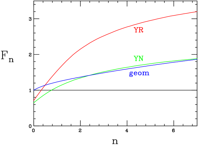
Figure 1: Yoshino-Rychkov (YR), Yoshino-Nambu (YN) and geometrical (geom) estimates of black hole formation factor.

II.2 Black Hole Cross Section

Adopting the Yoshino-Rychkov lower bound as an estimate of the black hole formation factor, and assuming again that $\sqrt{\hat{s}}=M_{\mbox{\scriptsize BH}}$, we obtain the parton-level cross section, shown as a function of the Planck scale for a 5 TeV black hole in Figure 2. For $n>2$ extra dimensions, the $n$-dependence of the formation factor tends to cancel that of the Schwarzschild radius, so that the cross section is not strongly dependent on the number of extra dimensions. Values of $n$ less than 3 are in any case strongly disfavoured on astrophysical grounds Hannestad:2001xi .

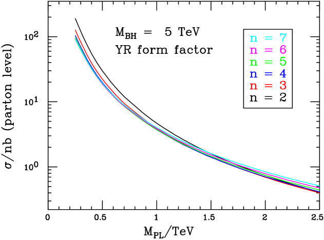
Figure 2: Parton-level black hole cross section.

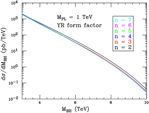
Figure 3: Hadron-level black hole cross section at the LHC.

To estimate the cross section for black hole production at a hadron collider, we must convolve the parton-level cross section with the parton distributions in the incident hadrons. The resulting cross section for a $pp$ collider at c.m. energy 14 TeV (i.e. the LHC) is shown in Figure 3. At the LHC design luminosity of $10^{34}$ cm^-2s^-1, this corresponds to more than one black hole per second with mass above 5 TeV.

II.3 Measuring the Planck Scale

If we accept the Yoshino-Rychkov result as a reliable estimate of the black hole formation factor, we see from Figures 2 and 3 that a measurement of the cross section for a given range of black hole masses would fix the Planck mass in a way that is substantially independent of the number of extra dimensions, at least in the astrophysically favoured region $n>2$.

Of course, one expects some dramatic changes in the cross section and final state at partonic c.m. energies around the Planck scale, due to the onset of strong gravitational scattering. However, to predict those changes one would need a quantum theory of gravity, so deducing the Planck mass from them would not be straightforward. Measurements well above the Planck scale, on the other hand, can reasonably be interpreted in a classical approximation, as we are doing here.

The problem in any case is to make a reliable measurement of the black hole mass, or more correctly the partonic c.m. energy for black hole formation. Since we do not observe the colliding partons, this can only be inferred from properties of the final state, which will be dominated by the decay of the black hole.

III BLACK HOLE DECAY

Although the formation of a horizon in parton collisions well above the Planck scale seems reliably established, the nature and fate of the object thus created is much less clear. The usual working hypothesis has been that the evolution of the system has four phases:

• Balding phase: all ‘hair’ (characteristics other than mass, charge and angular momentum) and multipole moments are lost through gravitational and Hawking radiation, and the object becomes the multidimensional generalization of a Kerr-Newman black hole. In fact any residual charge after this phase is probably negligible Giddings:2001bu , so the Kerr solution is assumed.

• Spin-down phase: the Kerr black hole loses angular momentum by Hawking radiation and becomes a Schwarzschild black hole.

• Schwarzschild phase: the black hole loses mass through Hawking radiation and its temperature rises until the mass and/or temperature reach the Planck scale.

• Planck phase: the object (‘string ball’?) is in the realm of quantum gravity and its fate cannot be predicted. It could decay into a few quanta with Planck-scale energies Giddings:2001bu , evaporate at the Hagedorn temperature Dimopoulos:2001qe , or even form a new kind of stable relic object Koch:2005ks .

At present, each of these decay phases is subject to great uncertainty. The amount of gravitational radiation emitted in the balding phase is of major concern because this constitutes missing energy that would spoil the connection between collision energy and black hole mass Yoshino:2005hi ; Anchordoqui:2003ug ; Cardoso:2005jq . In higher dimensions there are solutions to the Einstein equation that are not simply generalizations of the four-dimensional solutions, such as black rings Horowitz:2005rs . Probably there are more complicated objects still to be discovered. It is not clear whether such configurations would be able to spin down to the Schwarzschild solution, or what their Hawking radiation would look like. Even assuming the generalized Kerr solution, the amount and distribution of Hawking radiation during spin-down is still under investigation Harris:2005jx ; Duffy:2005ns ; Casals:2005sa ; Ida:2006tf .

In the Schwarzschild phase too there are many points that require further clarification. What fraction of the Hawking radiation is emitted as detectable Standard Model particles on the brane, and how much escapes into the bulk? Is the decay process too rapid for the relationship between black hole mass and temperature to remain valid throughout? Do secondary decays significantly distort the Hawking spectrum? And in the final Planck phase, what are the consequences of alternative models for the fate of the remnant object?

Many of these questions await theoretical answers, but some can be illuminated by numerical simulations. For the latter, we shall start with the hypotheses that practically all the energy of the parton collision goes into the black hole, that the decay is dominated by the Schwarzschild phase, and that the Hawking radiation consists entirely of Standard Model particles on the brane. With these assumptions, a detailed picture of the final state can be presented and the effects of some of the uncertainties can be investigated.

III.1 Hawking Spectrum

With the above assumptions, the spectrum of particles emitted during black hole decay takes the form

$$\frac{dN}{dE}\propto\frac{\gamma E^{2}}{(e^{E/T_{\mbox{\scriptsize H}}}\mp 1)}T_{\mbox{\scriptsize H}}^{n+6}$$ (8)

where as usual the $\mp$ applies to bosons and fermions, $T_{\mbox{\scriptsize H}}$ is the Hawking temperature

$$T_{\mbox{\scriptsize H}}=\frac{n+1}{4\pi r_{\mbox{\scriptsize S}}}\propto M_{\mbox{\scriptsize BH}}^{-\frac{1}{n+1}}$$ (9)

and $\gamma$ is a $(4+n)$-dimensional grey-body factor Harris:2004mf ; Ida:2002ez ; Kanti:2002nr ; Harris:2003eg . The latter takes account of the fact that the wave function of a particle created in the intense gravitational field near the horizon has to propagate through the curved space around the black hole in order for the particle to be observed. By detailed balance, the grey-body factor is equal to the absorption coefficient of the black hole for waves incident from infinity. For particles emitted at high energies the wavenumber is large compared with the curvature, so grey-body effects are small and the spectrum is close to black-body. But at low energy the emission is strongly modified in a way that depends on the spin and the number of extra dimensions.

Figures 4–6, taken from Harris:2004mf , show the grey-body factors for scalars, fermions and gauge bosons as functions of the particle energy in units of the inverse horizon radius. What is actually plotted here is the absorption cross section in units of $\pi r_{\mbox{\scriptsize S}}^{2}$, which tends to 4 at high energies. We see that the main effect in extra dimensions is the suppression of low-energy gauge boson emission.

\psfrag{x}[2.5]{$E\,r_{\mbox{\scriptsize S}}$}\psfrag{y}[2.5]{$\hat{\sigma}^{(0)}_{\mbox{\scriptsize abs}}/\pi r_{\mbox{\scriptsize S}}^{2}$}\includegraphics[width=506.45905pt]{ngrey0.ps}

Figure 4: Grey-body factors for scalar emission on the brane from a $(4+n)$D black hole.

\psfrag{x}[2.5]{$E\,r_{\mbox{\scriptsize S}}$}\psfrag{y}[2.5]{$\hat{\sigma}^{(1/2)}_{\mbox{\scriptsize abs}}/\pi r_{\mbox{\scriptsize S}}^{2}$}\includegraphics[width=506.45905pt]{ngrey05.ps}

Figure 5: Grey-body factors for fermion emission on the brane from a $(4+n)$D black hole.

\psfrag{x}[2.5]{$E\,r_{\mbox{\scriptsize S}}$}\psfrag{y}[2.5]{$\hat{\sigma}^{(1)}_{\mbox{\scriptsize abs}}/\pi r_{\mbox{\scriptsize S}}^{2}$}\includegraphics[width=506.45905pt]{ngrey1.ps}

Figure 6: Grey-body factors for gauge boson emission on the brane from a $(4+n)$D black hole.

III.2 Integrated Flux and Lifetime

Integrating the spectrum in Equation 8, including the grey-body factors, and multiplying by the number of Standard Model degrees of freedom for each spin, one obtains Harris:2004mf the total flux of particles of each type in black hole decay.

\psfrag{x}[2.5]{$n$}\psfrag{y}[2.5]{$F\,r_{\mbox{\scriptsize S}}$}\includegraphics[width=506.45905pt]{bhfluxp.ps}

Figure 7: Integrated flux of Hawking emission on the brane in the decay of a $(4+n)$D black hole.

Expressed in units of the inverse horizon radius, as shown in Figure 7, the particle fluxes are independent of the black hole mass and Planck scale. When the flux in these units exceeds unity, which we see is the case for $n>2$, the time between emissions is less than the time for a light-signal to travel a distance equal to the horizon radius. In these circumstances it is difficult to see how the emission can remain thermal. However, we shall continue to make that assumption in the absence of any better understanding.

Assuming that the Schwarzschild phase of decay is dominant, and that the mass and temperature are related by Equation 9 throughout (which we have just seen must be doubtful), the total energy flux can be integrated Harris:2005jx to find the time at which the entire mass of the black hole has been radiated away. This measure of the lifetime, expressed in units of the inverse of the initial mass, is shown in Figure 8. We see that the lifetime falls very steeply as a function of the number of dimensions, and indeed can be comparable with the inverse mass when $n>4$, even for masses well above the Planck scale. When this is the case, the object formed can no longer really be said to have an independent existence as a black hole.

\psfrag{x}[2.5]{$n$}\psfrag{y}[2.5]{$\tau\,M_{\mbox{\scriptsize BH}}$}\psfrag{w}[1.75]{$M_{\mbox{\scriptsize BH}}=5M_{\mbox{\scriptsize PL}}$}\psfrag{z}[1.75]{$M_{\mbox{\scriptsize BH}}=10M_{\mbox{\scriptsize PL}}$}\includegraphics[width=506.45905pt]{bhlife.ps}

Figure 8: Mean lifetime of a $(4+n)$D black hole.

IV EVENT SIMULATION

IV.1 CHARYBDIS Event Generator

The simulation program CHARYBDIS Harris:2003db generates black hole production and decay configurations assuming that all the partonic collision energy goes into the mass of the hole, and that the Schwarzschild decay phase dominates. The identities and momenta of the incoming partons and outgoing primary decay products are passed to the HERWIG Corcella:2000bw event generator via the Les Houches interface Boos:2001cv . HERWIG then handles all the QCD parton showering, hadronization and secondary decays.

Name	Description	Values	Default
MINMSS	Minimum mass of black holes (GeV)	$<\mbox{{MAXMSS}}$	5000.0
MAXMSS	Maximum mass of black holes (GeV)	$\leq\mbox{c.m. energy}$	c.m energy
MPLNCK	Planck mass (GeV)	$\leq\mbox{{MINMSS}}$	1000.0
TOTDIM	Total number of dimensions ($4+n$)	6–11	6
TIMVAR	Allow $T_{\mbox{\scriptsize H}}$ to change with time	LOGICAL	.TRUE.
MSSDEC	Choice of decay products	1–3	3
GRYBDY	Include grey-body effects	LOGICAL	.TRUE.
KINCUT	Use a kinematic cut-off on the decay	LOGICAL	.FALSE.
NBODY	Number of particles in remnant decay	2–5	2

Table 1: Main CHARYBDIS parameters.

The main parameters that control the operation of CHARYBDIS are summarized in Table 1. The first four are self-evident. The remaining five provide the means to study the effects of some of the uncertainties discussed earlier. TIMVAR causes the temperature of the black hole to be updated according to Equation 9 after each emission; otherwise it is frozen at the initial value. MSSDEC controls whether heavy particles are included in the Hawking radiation: MSSDEC=1 allows only light particle emission (up to and including $b$ quarks); MSSDEC=2 includes top quark, W and Z emission; MSSDEC=3 includes also Higgs boson emission.

The parameters KINCUT and NBODY determine how the evolution of the black hole is terminated. If KINCUT=.TRUE., termination occurs when the chosen energy for an emitted particle is ruled out by the kinematics of a two-body decay. At this point an isotropic NBODY decay is performed on the black hole remnant. The NBODY particles are chosen according to the same probabilities used for the first part of the decay. The selection is then accepted if charge and baryon number are conserved, otherwise a new set of particles is picked for the decay. In the alternative termination (KINCUT=.FALSE.) particles are emitted according to their Hawking energy spectra until $M_{\mbox{\scriptsize BH}}$ falls below MPLNCK; then an NBODY decay as described above is performed. Any chosen energies which are kinematically forbidden are simply discarded.

Figure 9: Primary photon spectrum from black holes with initial masses 5.0–5.5 TeV in $n=2$ extra dimensions. Dashed: neglecting time-variation of temperature. Dot-dashed: neglecting grey-body factors. Solid: including both.

Figure 9 illustrates the effects of grey-body factors and temperature variation on the energy distribution of primary photons. Both tend to harden the spectrum, shifting the peak towards higher energies. They also reduce the total number of photons emitted, the grey-body factor by suppressing soft photon emission and the temperature variation by reducing the lifetime of the black hole.

	Particle emissivity (%)
	GRYBDY=.TRUE.		GRYBDY=.FALSE.
Particle type	Generator	Theory	Generator	Theory
Quarks	63.9	61.8	58.2	56.5
Gluons	11.7	12.2	16.9	16.8
Charged leptons	9.4	10.3	8.4	9.4
Neutrinos	5.1	5.2	4.6	4.7
Photon	1.5	1.5	2.1	2.1
Z0	2.6	2.6	3.1	3.1
W+ and W-	4.7	5.3	5.7	6.3
Higgs boson	1.1	1.1	1.0	1.1

Table 2: Relative numbers of primary emissions from black holes with initial masses 5.0–5.5 TeV in $n=2$ extra dimensions..

Table 2 shows the relative numbers of primary particles of different types emitted when the parameters TIMVAR, GRYBDY, NBODY and NBODY have their default values, compared to the values obtained by integrating the theoretical spectra. The minor discrepancies are due mainly to kinematic constraints, particle masses and charge conservation.

IV.2 Event Characteristics

Turning from single-particle spectra to overall event characteristics, one interesting feature is that black hole decay is associated with large missing transverse energy, due to copious primary and secondary neutrino emission. Figure 10, from Harris:2004xt , shows a comparison with expected QCD and SUSY missing $E_{T}$ distributions generated using HERWIG Corcella:2000bw ; Moretti:2002eu . We see that the black hole missing $E_{T}$ is typically larger even than that in supersymmetric processes, where missing energy is mostly carried off by a pair of neutralinos. The effect is partly due to the larger mass of the black hole, relative to the assumed SUSY scale. However, a large cross section with large missing energy would clearly be a good initial indicator of black hole production.

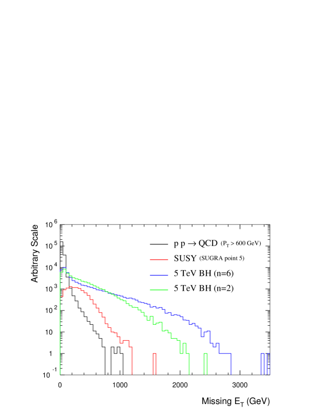
Figure 10: Missing transverse energy for various processes at the LHC.

IV.3 Measuring Black Hole Masses

The large missing energy in black hole decay poses a problem for the reconstruction of the mass of the black hole from its decay products. In Harris:2004xt we found that a cut on missing $E_{T}<100$ GeV was necessary for a useful mass resolution of around 4%, i.e. $\pm 200$ GeV at 5 TeV, as illustrated in Figure 11. At this low value of missing $E_{T}$, QCD background has to be controlled by requiring at least 4 high-$E_{T}$ jets.

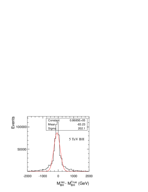
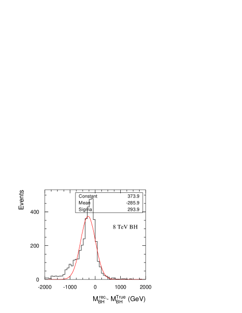
Figure 11: Black hole mass resolution after cuts.

V DETERMINING THE NUMBER OF EXTRA DIMENSIONS

V.1 Fitting Emission Spectra

In the event that black holes are produced at the LHC, the quantity of principal interest will be the number of extra dimensions, $n$. Given the sensitivity of the Hawking temperature to $n$ in Equation 9, it would seem that fitting the emission spectra for various black hole masses would allow one to extract this quantity Dimopoulos:2001hw . However, we found in Harris:2004xt that the theoretical uncertainties, together with the distortion of the spectrum by secondary decays, would make it difficult to have confidence in such a measurement.

For example, Figure 12 shows the effect of possible time variation of the Hawking temperature on a fit to the primary electron spectrum (assuming this could be unfolded cleanly from the data). For events generated with the temperature frozen (left), the fit gives a result consistent with the input value $n=2$, whereas re-thermalization between every emission (right) systematically shifts the fit to higher values, due to the higher average temperature. Since the true situation would presumably lie between these extremes, the true value of $n$ could not be extracted without a deeper understanding of the decay process.

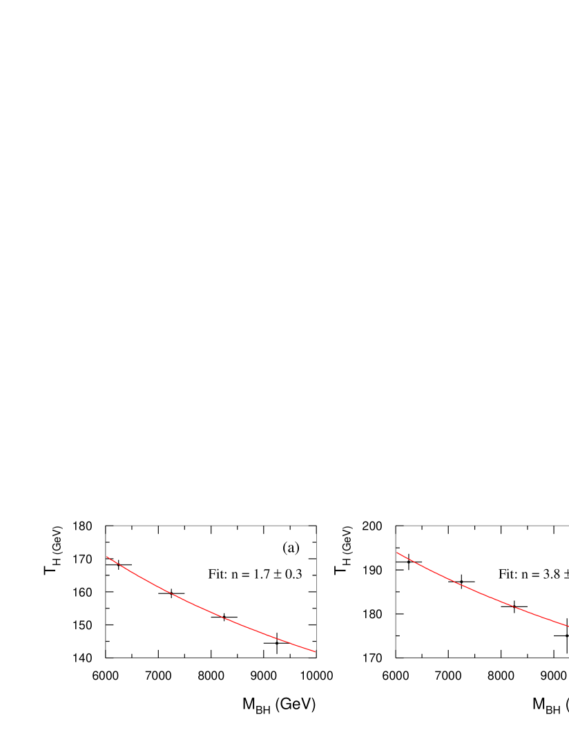
Figure 12: Fits to $T_{\mbox{\scriptsize H}}$ vs $M_{\mbox{\scriptsize BH}}$ from primary electron spectrum for $n=2$. (a) TIMVAR off; (b) TIMVAR on.

Figure 13 illustrates another difficulty in fitting the emission spectrum as a function of black hole mass, this time due to kinematic effects at higher energies. The limitation to emission energies less than half the total mass significantly truncates the spectrum generated according to Equation 8 at low masses and/or large values of $n$.

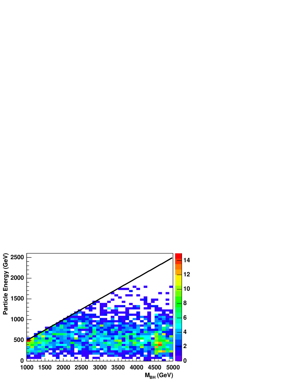
(a) $n=2$.

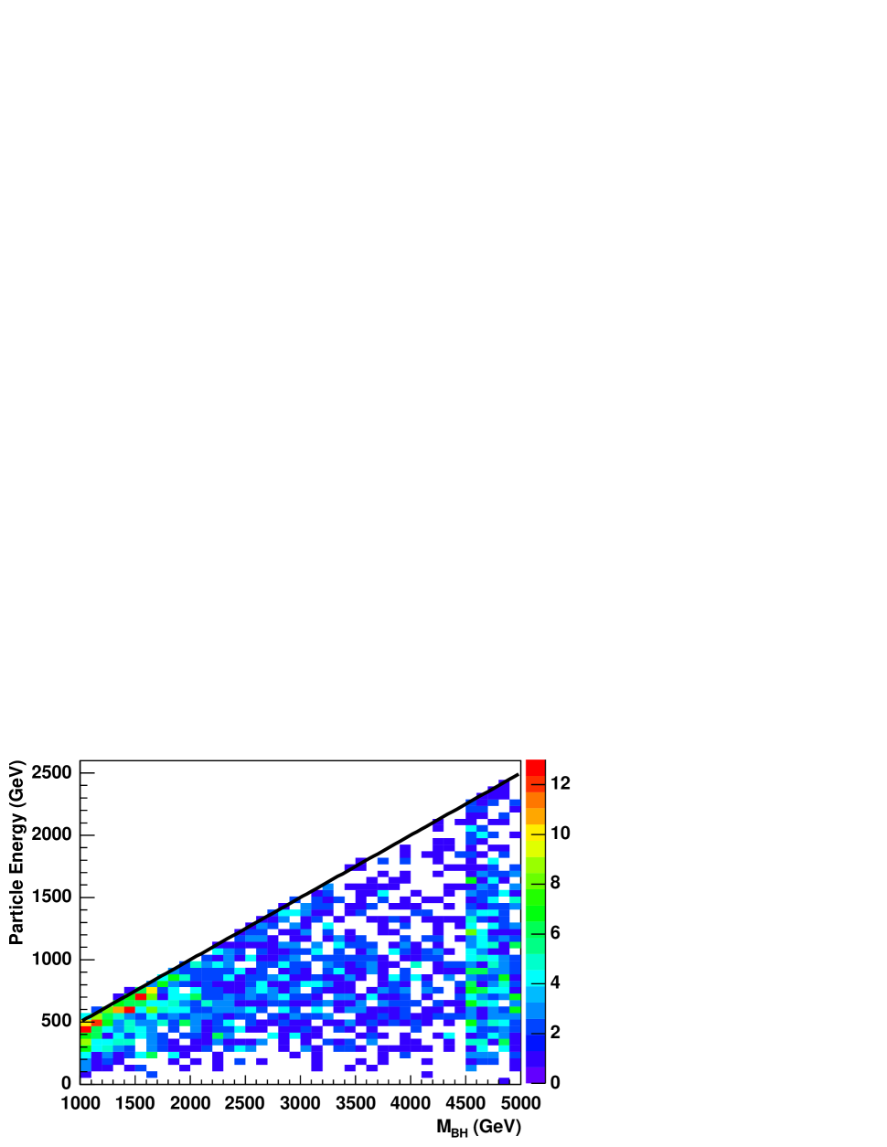
(b) $n=4$.

Figure 13: Energy distribution of primary decay products vs $M_{\mbox{\scriptsize BH}}$, showing the effect of the kinematic limit $E<M_{\mbox{\scriptsize BH}}/2$. The colour code indicates the number of particles in each bin per 1000 events.

V.2 A Possible Observable

In order to avoid the low-energy region of Hawking emission, where secondary decays distort the spectrum, and the highest energies where the kinematic cutoff takes effect, we examined Harris:2004xt the region of high but not extreme energies, $E\sim E_{\mbox{\scriptsize cut}}=M_{\mbox{\scriptsize BH}}/2-E_{d}$ where $E_{d}$ is a few hundred GeV. Particles in this region are also less sensitive to time variation of the temperature, since they tend to be emitted early in the evolution of the black hole. This tendency is further enhanced by demanding that the highest-energy emission should have energy $E_{\mbox{\scriptsize max}}>E_{\mbox{\scriptsize cut}}$. We therefore looked at the fraction $F$ of events satisfing this cut as a function of $M_{\mbox{\scriptsize BH}}$.

(a) Default case.

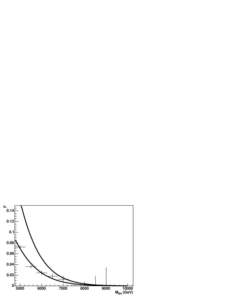
(b) No time variation.

(c) Kinematic cut on.

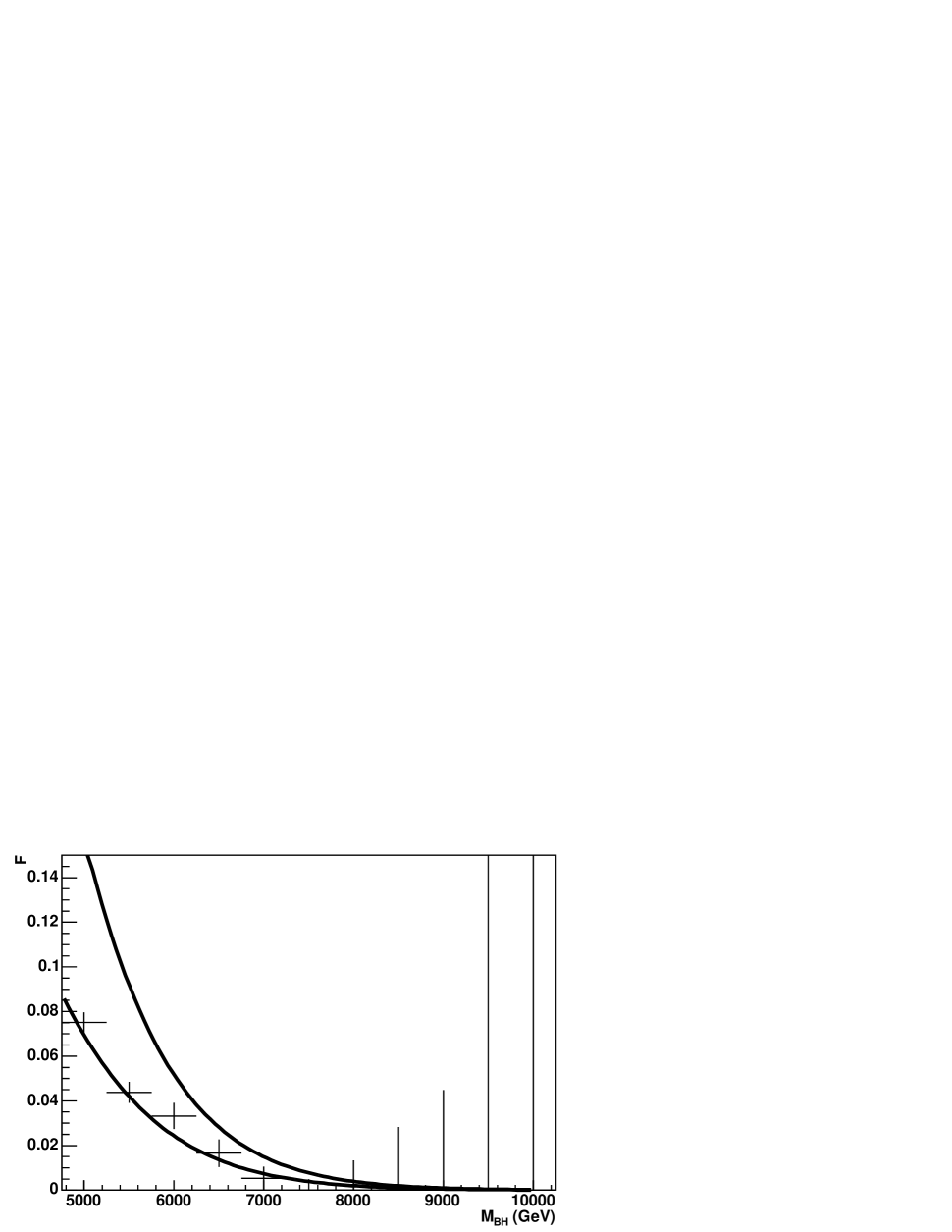
(d) 4-body remnant decay.

Figure 14: Fraction of events with $E_{\mbox{\scriptsize max}}>M_{\mbox{\scriptsize BH}}/2-400$ GeV vs $M_{\mbox{\scriptsize BH}}$ for different options, all with $n=4$. Upper and lower bounds explained in the text are also shown.

As shown in Figure 14, for $E_{d}=400$ GeV this observable is indeed relatively insensitive to the uncertainties represented by the CHARYBDIS parameters TIMVAR, KINCUT and NBODY. The upper and lower bounds were obtained by integrating the Planck spectrum from $E_{\mbox{\scriptsize cut}}$ up to infinity and up to $M_{\mbox{\scriptsize BH}}/2$, respectively, and include a $\pm 200$ GeV systematic uncertainty in the black hole mass. The value of $F$ always lies within, or at least is consistent with, the expected band. Therefore a fit to this observable should have less model dependence than analyses based, for example, on a fit to the full emission spectrum.

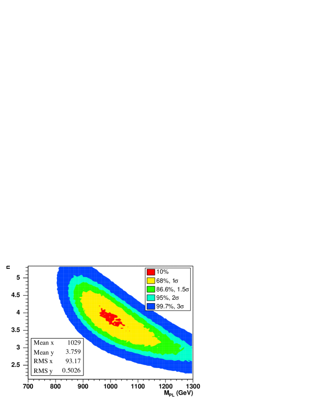
Figure 15: Combined measurement of Planck mass and number of extra dimensions.

In Harris:2004xt we combined a fit to this observable and a cross-section measurement with an assumed error of 20%, to make a joint determination of the Planck mass and the number of extra dimensions. As shown in Figure 15, for $M_{\mbox{\scriptsize PL}}=1$ TeV and $n=4$ the method gives an unbiased estimate of these quantities, with $1\sigma$ errors of $\Delta M_{\mbox{\scriptsize PL}}/M_{\mbox{\scriptsize PL}}\sim 15\%$, $\Delta n\sim 0.75$ (strongly correlated).

VI CONCLUSIONS

If there are indeed extra dimensions large and numerous enough to reduce the fundamental Planck scale to the TeV range, black hole production at accelerators, with substantial cross sections, is a real possibility. Such a discovery would arguably be the most profound advance in fundamental physics since general relativity. It would also constitute the first observation of Hawking radiation. However, as I have repeatedly emphasised, there remain many uncertainties about the precise nature, evolution and ultimate fate of the objects that would be formed. The strategy adopted here has been to start with a crude but flexible simulation framework, and to look for observables that are less sensitive to some of these uncertainties, in order to stimulate thinking about how the fundamental parameters could be measured. If real data on this process do become available, there will undoubtedly be an explosion of theoretical and experimental activity that will rapidly reduce the uncertainties.

- (1) S. B. Giddings and S. D. Thomas, “High energy colliders as black hole factories: The end of short distance physics,” Phys. Rev. D 65, 056010 (2002) [arXiv:hep-ph/0106219].
- (2) S. Dimopoulos and G. Landsberg, “Black holes at the LHC,” Phys. Rev. Lett. 87, 161602 (2001) [arXiv:hep-ph/0106295].
- (3) I. Antoniadis, “A Possible New Dimension At A Few Tev,” Phys. Lett. B 246, 377 (1990); N. Arkani-Hamed, S. Dimopoulos and G. R. Dvali, “The hierarchy problem and new dimensions at a millimeter,” Phys. Lett. B 429, 263 (1998) [arXiv:hep-ph/9803315]; I. Antoniadis, N. Arkani-Hamed, S. Dimopoulos and G. R. Dvali, “New dimensions at a millimeter to a Fermi and superstrings at a TeV,” Phys. Lett. B 436, 257 (1998) [arXiv:hep-ph/9804398].
- (4) L. Randall and R. Sundrum, “A large mass hierarchy from a small extra dimension,” Phys. Rev. Lett. 83, 3370 (1999) [arXiv:hep-ph/9905221].
- (5) H. Yoshino and Y. Nambu, “Black hole formation in the grazing collision of high-energy particles,” Phys. Rev. D 67, 024009 (2003) [arXiv:gr-qc/0209003].
- (6) D. M. Eardley and S. B. Giddings, “Classical black hole production in high-energy collisions,” Phys. Rev. D 66, 044011 (2002) [arXiv:gr-qc/0201034].
- (7) H. Yoshino and V. S. Rychkov, “Improved analysis of black hole formation in high-energy particle collisions,” Phys. Rev. D 71, 104028 (2005) [arXiv:hep-th/0503171].
- (8) C. M. Harris, M. J. Palmer, M. A. Parker, P. Richardson, A. Sabetfakhri and B. R. Webber, “Exploring higher dimensional black holes at the Large Hadron Collider,” JHEP 0505, 053 (2005) [arXiv:hep-ph/0411022].
- (9) C. M. Harris, “Physics beyond the standard model: Exotic leptons and black holes at future colliders,” Cambridge Ph.D. thesis, arXiv:hep-ph/0502005.
- (10) D. Ida, K. y. Oda and S. C. Park, “Rotating black holes at future colliders: Greybody factors for brane fields,” Phys. Rev. D 67, 064025 (2003) [Erratum-ibid. D 69, 049901 (2004)] [arXiv:hep-th/0212108].
- (11) S. Hannestad and G. G. Raffelt, “Stringent neutron-star limits on large extra dimensions,” Phys. Rev. Lett. 88, 071301 (2002) [arXiv:hep-ph/0110067]; “Supernova and neutron-star limits on large extra dimensions reexamined,” Phys. Rev. D 67, 125008 (2003) [Erratum-ibid. D 69, 029901 (2004)] [arXiv:hep-ph/0304029].
- (12) S. Dimopoulos and R. Emparan, “String balls at the LHC and beyond,” Phys. Lett. B 526, 393 (2002) [arXiv:hep-ph/0108060].
- (13) B. Koch, M. Bleicher and S. Hossenfelder, “Black hole remnants at the LHC,” arXiv:hep-ph/0507138.
- (14) L. A. Anchordoqui, J. L. Feng, H. Goldberg and A. D. Shapere, “Inelastic black hole production and large extra dimensions,” Phys. Lett. B 594, 363 (2004) [arXiv:hep-ph/0311365].
- (15) V. Cardoso, E. Berti and M. Cavaglia, “What we (don’t) know about black hole formation in high-energy collisions,” Class. Quant. Grav. 22, L61 (2005) [arXiv:hep-ph/0505125].
- (16) G. T. Horowitz, “Higher dimensional generalizations of the Kerr black hole,” arXiv:gr-qc/0507080.
- (17) C. M. Harris and P. Kanti, “Hawking radiation from a (4+n)-dimensional rotating black hole,” arXiv:hep-th/0503010;
- (18) G. Duffy, C. Harris, P. Kanti and E. Winstanley, “Brane decay of a (4+n)-dimensional rotating black hole: Spin-0 particles,” JHEP 0509, 049 (2005) [arXiv:hep-th/0507274].
- (19) M. Casals, P. Kanti and E. Winstanley, “Brane decay of a (4+n)-dimensional rotating black hole. II: Spin-1 particles,” arXiv:hep-th/0511163.
- (20) D. Ida, K. y. Oda and S. C. Park, “Rotating black holes at future colliders. III: Determination of black hole evolution,” arXiv:hep-th/0602188.
- (21) P. Kanti and J. March-Russell, “Calculable corrections to brane black hole decay. I: The scalar case,” Phys. Rev. D 66, 024023 (2002) [arXiv:hep-ph/0203223]; “II: Greybody factors for spin 1/2 and 1,” Phys. Rev. D 67, 104019 (2003) [arXiv:hep-ph/0212199];
- (22) C. M. Harris and P. Kanti, “Hawking radiation from a (4+n)-dimensional black hole: Exact results for the Schwarzschild phase,” JHEP 0310, 014 (2003) [arXiv:hep-ph/0309054].
- (23) C. M. Harris, P. Richardson and B. R. Webber, “CHARYBDIS: A black hole event generator,” JHEP 0308, 033 (2003) [arXiv:hep-ph/0307305].
- (24) G. Corcella et al., “HERWIG 6: An event generator for hadron emission reactions with interfering gluons (including supersymmetric processes),” JHEP 0101, 010 (2001) [arXiv:hep-ph/0011363]; “HERWIG 6.5 release note,” arXiv:hep-ph/0210213.
- (25) E. Boos et al., “Generic user process interface for event generators,” arXiv:hep-ph/0109068.
- (26) S. Moretti, K. Odagiri, P. Richardson, M. H. Seymour and B. R. Webber, “Implementation of supersymmetric processes in the HERWIG event generator,” JHEP 0204, 028 (2002) [arXiv:hep-ph/0204123].