Scalar Mesons in B-decays

Abstract

We summarize some persistent problems in scalar spectroscopy and discuss what could be learned here from charmless B-decays. Recent experimental results are discussed in comparison with theoretical expectations: a simple model based on penguin dominance leads to various symmetry relations in good agreement with recent data; a factorisation approach yields absolute predictions of rates. For more details, see talk .

1 WHY STUDYING SCALARS IN B-DECAYS

There are various reasons for studying scalar particles in B-decays:

1. Dominance of $S$-wave resonances with little background from crossed channels
In $(B\to 1,2,3)$-decays the masses of (1,2) resonances can extend to $M\mathrel{\mathop{\kern 0.0pt\hbox to0.0pt{\raise 0.86108pt\hbox{$<$}\hss}}\lower 3.87495pt\hbox{\kern-1.90002pt$\sim$}}5$ GeV. Then there is little overlap with resonances in crossed channels (2,3) or (1,3). This is very different from $D$ decays where resonance masses extend only up to $\sim 1.5$ GeV and in general there is a large overlap. Furthermore, in the final 2-body systems $S$-wave interactions are dominant.

2. New source of glueballs

The elementary subprocess $b\to sg$ with an isolated gluon is rather well understood theoretically and is described by a penguin diagram. The decay rate has been calculated in next-to-leading order of perturbative QCD as greub

$${B}(b\to sg)=(5\pm 1)\times 10^{-3}.$$ (1)

The gluon may give rise to production of a glueball which could show up as a resonance in the system $X$ of 2-body decays $B\to K^{(*)}+X$. This process adds to the other well known gluon rich processes like: central production in $pp$ collisions, $J/\psi\to\gamma X$ and $p\bar{p}$ annihilation near threshold.

3. Non-charm final states with strangeness
The decays $b\to sq\bar{q}$ are dominated again by the gluonic penguin process whereas the electroweak tree diagrams occur at the level of 20% only. In the leading penguin approximation the decays $b\to su\bar{u},\ sd\bar{d},\ ss\bar{s}$ occur with the same fraction and have been calculated to amount to $\sim 2\times 10^{-3}$ each. In the corresponding hadronic 2-body final states $B\to xy$, if $x$ and $y$ are members of $SU(3)$ multiplets $X,Y$ each, one obtains various symmetry relations mo1 . Hopefully, this will ultimately identify the members of the lightest scalar nonet and the mixing properties.

2 PROBLEMS OF LIGHT SCALAR MESON SPECTROSCOPY

The interest in light scalar mesons originates from the following expectations:
1. The existence of glueballs
This is a requirement from the first days of QCD and may be the most urgent open problem of the theory at the fundamental level. In lattice QCD, quenched approximation, the lightest glueball appears in the $0^{++}$ channel with a mass of 1400-1800 MeV bali . The effect of unquenching is under study but realistic estimates are still difficult, especially because of the large quark masses. An alternative QCD approach is based on QCD sum rules narison where the lightest glueball is centered around 1000-1400 MeV.

2. Multiplets of $q\bar{q}$ and exotic bound states
There is no general consensus on the members of the lightest $q\bar{q}$ nonet, i.e. the parity partner of $\pi,K,\eta,\eta^{\prime}$. In addition, there is the possibility of tetraquarks jaffe , bound states of di-quarks.

The list of scalar particles provided by the PDG pdg with mass $M\mathrel{\mathop{\kern 0.0pt\hbox to0.0pt{\raise 0.86108pt\hbox{$<$}\hss}}\lower 3.87495pt\hbox{\kern-1.90002pt$\sim$}}1.8$ GeV includes
$I=0$: $f_{0}(600)$ (or $\sigma$), $f_{0}(980)$, $f_{0}(1370)$, $f_{0}(1500)$, $f_{0}(1710)$;
$I=\frac{1}{2}$: $\kappa(900)$ (?), $K^{*}_{0}(1430)$;
${I=1}$: $a_{0}(980)$, $a_{0}(1450)$.

There are two typical scenarios for the classification of these states:

I. One nonet below and one above 1 GeV
The nonet of lower mass includes $\sigma,\ \kappa,\ f_{0}(980),\ a_{0}(980)$, either $q\bar{q}$ (see, for example, Ref. morgan and Van Beveren conf ) or $qq\bar{q}\bar{q}$ jaffe bound states. The higher mass states could then make a $q\bar{q}$ nonet with members $K^{*}_{0}(1430)$ and $a_{0}(1450)$; in the isoscalar sector the three states $f_{0}(1370)$, $f_{0}(1500)$ and $f_{0}(1710)$ could be, as originally proposed in amsler , a superposition of the glueball and the two members of the isoscalar nonet.

II. One nonet above 1 GeV
In this scheme the $\sigma$ and $\kappa$ with the parameters given are not considered as physical states to be classified along the lines we discuss here. The $q\bar{q}$ nonet is rather formed by $a_{0}(980)$ (or also $a_{0}(1450)$), $f_{0}(980)$, $K^{*}_{0}(1430)$ and $f_{0}(1500)$ klempt ; mo2 whereas two higher mass nonets including $f_{0}(1370)$ have been proposed in anisovich . The $\pi\pi$ $S$-wave is interpreted as being dominated by a very broad object, centered around 1 GeV, the lower part could be responsible for the $\sigma(500)$ effect. This broad state ($\Gamma>500$ MeV) has been proposed as representing the isoscalar glueball by various arguments anisovich ; mo2 .

There are states whose identity is in doubt as can be seen by the large uncertainty in mass and width estimated by the PDG: $\sigma(500)$, $f_{0}(1370)$ with no single branching ratio or ratio of such numbers accepted by PDG and finally $\kappa$ or $K^{*}(800)$ not carried in the main listing of PDG. We will add a few remarks on these problematic states which will be of relevance for our discussion of $B$ decays.

2.1 Isoscalar channel: $f_{0}(600)$ or $\sigma$ and $f_{0}(1370)$

Most definitive experimental results on these states can be obtained from the $2\to 2$ scattering processes $\pi\pi\to\pi\pi,K\bar{K},\eta\eta$ applying an energy independent partial wave analysis (EIPWA); in this case unitarity provides important constraints in the full energy range. Recently, results on $D$ and $B$ decays as well as $p\bar{p}\to 3$ particles with higher statistics became available. There is no general constraint on the mass dependence of the amplitude which can be affected by various dynamical effects. So far, in these processes no EIPWA over the full energy range has been performed, so an optimal description of data for a particular model parametrization is selected. A promising new approach towards EIPWA in $D$-decays has been presented at this conference by Meadows meadows .

Concerning the $\pi\pi$ interaction there is a general consensus that there exists indeed a broad state with the width of the order of the mass, but the parameters depend on the mass range considered, a feature which is known already since about 30 years.

1. Low mass range $M_{\pi\pi}\mathrel{\mathop{\kern 0.0pt\hbox to0.0pt{\raise 0.86108pt\hbox{$<$}\hss}}\lower 3.87495pt\hbox{\kern-1.90002pt$\sim$}}0.9\ldots 1.2$ GeV.
In this region the complex $\pi\pi$ amplitude moves along the unitarity circle to its top (phase $90^{\circ}$) where a rapid circular motion follows from $f_{0}(980)$. An early analysis has been performed by the Berkeley collaboration protopopescu , they found a state, $\sigma$, with $M_{\sigma}=660\pm 100$ MeV, $\Gamma_{\sigma}=640\pm 140$ MeV. Recently, results from $D$-decays by E791 e791 , FOCUS focus and from $J/\psi\to\omega\pi\pi$ by BES bes have been interpreted in terms of a $\sigma$ with similar mass, although good fits based on a $K$ matrix parametrization have been obtained without such a state focus . On the theoretical side, parametrizations of such data using the low mass $\chi PT$ constraints lead to a low mass pole with $M_{\sigma}\sim 450$ MeV and $\Gamma_{\sigma}\sim 450\ldots 600$ MeV (see, e.g. Refs. oop ; cgl and the reports by Bugg and Pelaes conf1 ).

2. Extended mass range $500\leq M\leq 1800$ MeV
In case of a broad state the parameters should be determined from the energy interval where its influence is important and this includes the inelastic region above 1 GeV.

All analyses of $\pi\pi$ scattering in this region find again one broad state, but with a higher mass than before, in a range around 1000 MeV and with large width $>500$ MeV. The first analysis along these lines goes back again 30 years hyams and in Table 1 we list the pole positions from K matrix fits of various analyses. The fits by Estabrooks estabrooks refer to the four solutions of an EIPWA of elastic $\pi\pi$ scattering em as well as of the $\pi\pi\to K\bar{K}$ reaction. In all solutions of the EIPWA the $S$-wave amplitude above 1 GeV follows a circular path with some inelasticity in the Argand diagram ( $Im\ T$ vs. $Re\ T$) which can be fitted by a broad resonance. Superimposed is a smaller circle corresponding to a resonance estabrooks with parameters close to what is known today as $f_{0}(1500)$. No additional pole, such as $f_{0}(1370)$, is seen in this analysis. A similar picture is found mo2 for the inelastic channels $\pi\pi\to\eta\eta$ and $\pi\pi\to K\bar{K}$ comprising the broad background and $f_{0}(1500)$ with the interference pattern

$$\pi\pi\to K\bar{K}$$: background - constructive interference

background - destructive interference

(2)

This broad state is seen in a variety of processes and has been dubbed $f_{0}(1000)$ in amp . Later arguments have been presented that this broad state be a glueball anisovich ; mo2 . This state also appears in decay processes although it may happen that the higher mass tails are suppressed for dynamical reasons. As an example, we quote the study by BES beskk of the final state $J/\psi\to\omega K^{+}K^{-}$ where the large $S$-wave background (“$\sigma$”) extends up to about 2 GeV. A significant flat background has also been observed recently in the gluon rich channel $J/\psi\to\gamma K\bar{K}$ by BES besgammakk .

Apparently, the state $f_{0}(1370)$ shows up if reactions other than (1)-(3) in Table 1 without unitarity constraints are included in the fits. Whereas $f_{0}(980)$, $``f_{0}(1000)$” and $f_{0}(1500)$ are clearly seen as circles in the Argand diagrams, no such circle has ever been shown to exist for $f_{0}(1370)$. Before such a behaviour is demonstrated, this state could hardly be considered as established. The strong interference between background and $f_{0}(1500)$, leads to very different mass spectra, depending on the relative phase, which could easily simulate a “new state” $f_{0}(1370)$.

Authors	mass (MeV)	width (MeV)	channels
CERN-Munich hyams	1049	500	1
Estabrooks estabrooks	750	800-1000	1,2
Au, Morgan & Pennington amp	910	700	1,2,5
Anisovich and Sarantsev anisovich	1530	1120	1,2,3,4

Table 1: Position of broad state in the $T$ matrix of $\pi\pi$ scattering according to various K matrix fits to data from reactions (1) $\pi\pi\to\pi\pi$, (2) $\pi\pi\to K\bar{K}$, (3) $\pi\pi\to\eta\eta,\eta\eta^{\prime}$, (4) $p\bar{p}$ annihilation and (5) $J/\psi$ decays

We conclude that there is indeed a broad state in the isoscalar channel with decays into various 2-body final states but there is no standard form for its line shape. Different results on its mass emerge depending on whether the analytic parametrization is fitted to a small or a large mass range (corresponding to either a half resonance circle or an almost full circle) leading either to $\sigma(500)$ or “$f_{0}(1000)$”. There can be little doubt that both results refer to the same state. Studies along path 1 should ultimately extend their parametrization to include higher mass inelastic channels, especially the EIPWA results by Estabrooks, whereas the analyses along path 2 should include the very low mass $\pi\pi$ data as well.

2.2 Isospin $I=\frac{1}{2}$ channel: $\kappa(800)$ and $K^{*}_{0}(1430)$

The elastic $K\pi$ scattering up to 1700 MeV has been studied some time ago by an experiment at SLAC slac and the LASS experiment lass . The $S$ wave phase shifts have been parametrized in terms of $K^{*}_{0}(1430)$ with a small inelasticity $<10\%$ starting only above the inelastic threshold $M_{K\pi}\mathrel{\mathop{\kern 0.0pt\hbox to0.0pt{\raise 0.86108pt\hbox{$>$}\hss}}\lower 3.87495pt\hbox{\kern-1.90002pt$\sim$}}M_{K\eta^{\prime}}\sim 1450$ MeV and a slowly varying background with an effective range formula. This background phase in the considered range does not exceed about 50^∘ and insofar it is a phenomenon quite different from the background in $\pi\pi$ scattering where the background phase reaches 90^∘ below the first scalar resonance $f_{0}(980)$. We do not want to enter here into the discussion about a possible state $\kappa$ but point to different characteristics of the $K\pi$ amplitude in elastic scattering and decay relevant to our later discussion. For a theoretical analysis, see Büttiker et al. buttiker .

In weak decays like $D\to K\pi\mu\nu$ the $K\pi$ phase equals the one in elastic scattering according to the Watson theorem and this is nicely born out by the data (FOCUS goebel ). If rescattering effects are small, then the Watson theorem is still applicable in purely hadronic decays and a recent example for this behaviour is $B\to J/\psi K\pi$ measured by BaBar babarkpi . On the other hand, in $D\to K\pi\pi$ the $K\pi$ phases determined by E791 meadows follow the trend as in elastic scattering below the inelastic $K\eta^{\prime}$ threshold $M\sim 1400$ MeV, but with a relative shift of about 70^∘. The Argand diagram in Fig. 1) shows that the resonance circle related to $K^{*}_{0}(1430)$ is much smaller than the circle related to the background, which contrasts to elastic scattering with circles of comparable radii. Therefore the LASS parametrization does not represent the decay amplitude in an energy region beyond 1400 MeV.

Figure 1: Energy independent partial wave analysis of the $I=\frac{1}{2}$ $K\pi$ $S$-wave using E791 data “$c_{i}$” and form factors $F_{Di}$ meadows . Plotted are the rescaled quantities $S_{i}=c_{i}F_{Di}\frac{q}{\sqrt{s}}$ (arbitrary units) to be compared with the elastic unitarity circle for $K\pi\to K\pi$ scattering.

3 $B$-decays: experimental results on scalars

The $B$ branching ratios for the following scalar particles have been measured, for later comparison we present the results corrected for unseen channels, all in units of $10^{-6}$.

Isospin I=1: $a_{0}(980)$
So far only upper limits have been reported by BaBar babara0 , see Tab. 2.

$B^{0}\to K^{0}a^{0}_{0}$	¡ 9.2		$B^{+}\to K^{+}a^{0}_{0}$	¡ 2.9
$B^{0}\to K^{+}a^{-}_{0}$	¡  2.4		$B^{-}\to\bar{K}^{0}a^{-}_{0}$	¡ 4.6

Table 2: $B$ decays into $a_{0}(980)$ babara0 corrected using $B(a_{0}\to\eta\pi)=0.85$; all numbers $\times 10^{-6}$.

Isospin $I=\frac{1}{2}:K^{*}_{0}(1430)$
Total decay rates derived from BaBar babarkst and Belle data bellekst are given in Tab. 3.

	BaBar babarkst	Belle bellekst
$B^{0}\to K^{*0}_{0}\pi^{0}$	$12.7\pm 5.0$	$9.8\pm 2.7$
$B^{0}\to K^{*+}_{0}\pi^{-}$	$36.1\pm 12.2$	$16.4\pm 5.3$
$B^{+}\to K^{*0}_{0}\pi^{+}$	$37.0\pm 4.4$	(I) $45^{+15.3}_{-11.1}$   (II) $8.3^{+3.9}_{-2.6}$

Table 3: $B$ decays into $K^{*}_{0}(1430)$ corrected for unseen modes using $B(K^{*}_{0}\to K\pi)=0.93$; units in $10^{-6}$

Belle, in a full Dalitz plot analysis using an isobar model ansatz finds two quite different solutions in $B^{+}\to K^{*0}_{0}\pi^{+}$ corresponding to different interferences with a coherent background amplitude. Babar is inserting the LASS parametrization for the $K\pi$ phase in a larger energy interval up to $M\sim M_{D}$ and is then left with only one solution. As discussed above for $D\to K\pi\pi$ the behaviour of the $K\pi$ amplitude above 1400 MeV could be quite different from elastic scattering and a more general ansatz in this mass region seems appropriate. The situation is quite analogous to $f_{0}(980)$ in $\pi\pi$ interactions where the interference pattern of $f_{0}$ and background changes from one reaction to another. It will be therefore important to clarify the existence of two solutions and to possibly exclude one of them by physical arguments.

Isospin I=0: $f_{0}(1500)$
Both Belle bellekst and BaBar babarkk see a peak in the $K^{+}K^{-}$ Mass spectrum in $B\to(K^{+}K^{-})K$. The mass and width are consistent with $f_{0}(1500)$. However, no signal in the corresponding $\pi\pi$ decay channel is observed despite the ratio of branching ratios $\Gamma(f_{0}\to K\bar{K})/\Gamma(f_{0}\to\pi\pi)=0.241\pm 0.028$ pdg is favourable for the $\pi\pi$ channel. Therefore both collaborations suggested the existence of a new state, $f_{X}(1500)$ or $X(1500)$.

In a previous work mo1 studying the Belle data bellekst we argued that these phenomena are naturally explained by the existence of a broad background which interferes with $f_{0}(1500)$: constructively in $K^{+}K^{-}$ giving rise to the observed peak but destructively in $\pi^{+}\pi^{-}$ leading to a vanishing signal. In our analysis we have represented the mass spectra as a superposition of three components $f_{0}(980),\ f_{0}(1500)$ and a broad resonance as background, which fits the data well, see Figs. 2,3. This interference pattern is the same as in inelastic $\pi\pi\to K\bar{K},\eta\eta$ mo2 and elastic $\pi\pi$ scattering estabrooks (see above).

These signs are consistent with our hypothesis mo2 that the background represents a broad glueball (flavour singlet) with mass in the 1 GeV region or above interfering with $f_{0}(1500)$, which is close to a flavour octet state according to the considerations in klempt ; mo2 .

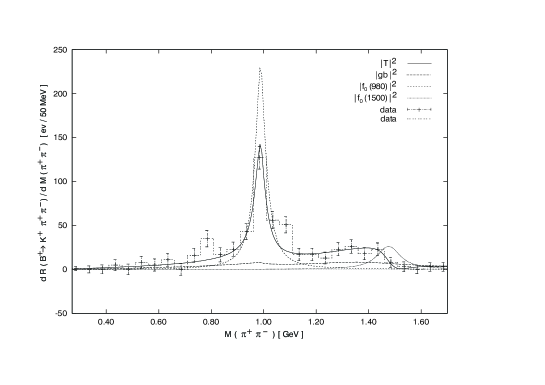
Figure 2: $\pi^{+}\pi^{-}$ mass spectrum in $B$-decays (BELLE bellekst ) in comparison with a model including $f_{0}(980),\ f_{0}(1500)$ and a broad glueball ($gb$). Also shown are the individual resonance terms. The background ($gb$) in this fit interferes destructively with both $f_{0}(980)$ and $f_{0}(1500)$.

Figure 3: $K^{+}K^{-}$ mass spectrum in $B$-decays (BELLE bellekst ) in comparison with the model amplitude, see Fig. (2). Here $f_{0}(1500)$ interferes constructively with the background.

Both collaborations find two solutions for the $B\to Kf_{0}(1500)$ rate corresponding to different interference signs with the background. From the total charmless and the partial fractions we obtain the branching ratios in Tab. 4. According to our model Sol. II is the physical solution.

$B(B\to f_{0}(1500)K)$	Belle ($B^{+}$)	BaBar $(B^{0})$
Sol. I ($bg-f_{0})$	$471.8\pm 51.3$	$223\pm 42$
Sol. II ($bg+f_{0})$	$61.1\pm 14.4$	$29.9\pm 13.7$

Table 4: $B$-decay rates ($\times 10^{-6}$) into $f_{0}(1500)K$ (total rates using $B(f_{0}(1500)\to K^{+}K^{-})=0.043$).

Isospin I=0: $f_{0}(980)$
$f_{0}(980)$ was the first scalar particle observed in $B$-decays and the results obtained by the heavy flavor averaging group (HFAG) hfag are presented in Tab. 5. In these decay channels there is again some background contribution as in case of $f_{0}(1500)$, so we expect two possible solutions corresponding to different interference signs. Note the negative interference in our fits in Figs. 2,3, also observed in $J/\psi\to\phi\pi\pi$ by DM2 dm2 . It would be important to study the possibility of a second solution besides the one in Tab. 5.

Other results on scalars
$f_{0}(1370)$: A $2\sigma$ signal has been observed by Belle bellekst , not so by BaBar babarkst .

$\sigma(600)$: No obvious peak near threshold is visible as in $D\to 3\pi$. For our discussion of scalars it would be interesting to obtain the rate for $B\to\sigma K$ (or a limit).

$\kappa(800):$ A $K\pi$ background in $K\pi\pi$ has been observed by Belle bellekst but a fit with a $\kappa$ particle was not successful.

$a_{0}(1450)$: This state has not been seen yet.

	$f_{0}(980)\to\pi\pi$	$f_{0}(980)\to all$
$B(B^{+}\to f_{0}(980)K^{+})$	$13.2\pm 1.6$	16.5
$B(B^{0}\to f_{0}(980)K^{0})$	$8.25\pm 1.5$	10.3

Table 5: $B$-decay rates ($\times 10^{-6}$) into $f_{0}(980)K$, for $f_{0}(980)\to\pi\pi$ and total rate using $\Gamma(f_{0}(980)\to\pi\pi)/\Gamma_{tot}\sim 0.8$.

4 $B$-decays into scalars: theoretical expectations

The theoretical considerations to some extent follow the ideas developed earlier for $B$-decays into pseudoscalar (P) and vector (V) particles. We outline here two complementary approaches.

4.1 Phenomenological amplitudes

The decay rates are expressed in terms of a set of phenomenological amplitudes including the gluonic penguin, the electroweak tree amplitudes and others. Such a scheme has been successfully applied to the decays $B\to PP,PV$ cr1 ; lipkin .

Here we apply a scheme of this kind mo1 , but in this exploratory phase for scalars with moderate statistics we restrict ourselves to including only the dominant penguin diagrams and neglect in particular the tree diagrams which give rise to corrections at the 20% level. We then consider in this scheme the three $q\bar{q}$ processes with the same amplitude as well as the gluonic amplitude

$$b\to su\bar{u},\quad b\to sd\bar{d},\quad b\to ss\bar{s},\quad b\to sg.$$ (3)

These processes together with the recombination of the spectator quark give rise to 2-body decays $B\to xy$ where $x,y$ are mesons out of the flavour $U(3)$ nonets $A$ and $B$. Given the members of these multiplets with a particular mixing angle the decay amplitudes can be given in terms of the following parameters: the penguin amplitude $p_{AB}$ with $s\to x$, the exchange amplitude $\beta_{AB}p_{AB}$ for $s\to y$ and $\gamma_{AB}p_{AB}$ for the gluonic amplitude. For a more detailed discussion, see Ref. mo1 , here we just adress for illustration the decay $B^{+}\to\eta^{\prime}K^{*+}$ for the mixing $\eta^{\prime}=(u\bar{u},d\bar{d},2s\bar{s})/\sqrt{6}$. The decay amplitude is derived from the penguin amplitudes as in Fig. 4 and reads

$$T=\frac{1}{\sqrt{6}}(1+2\beta_{PV}+4\gamma_{PV})p_{PV}$$ (4)

A consequence of this penguin dominance model are various symmetry relations, especially the $I=\frac{1}{2}$ rule: The final state of processes (3) has $I=0$ and therefore the final state of $B$ decay has the isospin of the spectator, for $B^{\pm},B^{0}$ this is $I=\frac{1}{2}$, which is also realized in our amplitudes mo1 , see also Tab. 6 below.

Figure 4: Two-body decay $B^{-}\to K^{-}\eta^{\prime}$ (or $B^{-}\to K^{*-}\eta^{\prime}$) with three amplitudes from (3): (a) amplitude $p^{u}_{K^{-}\eta^{\prime}}$ with $s\to K^{-}$, (b) exchange amplitude $p^{s}_{\eta^{\prime}K^{-}}$ with $s\to\eta^{\prime}$ and (c) amplitude $s_{K^{-}\eta^{\prime}}$ for gluonic production of $\eta^{\prime}$.

4.1.1 Application to $B$-decays into pseudoscalars

As a test of this penguin dominance model we have compared first with data on the decays $B\to PP,\ B\to PV$ mo1 . In Tab. 6 this comparison is repeated with new data compiled by HFAG hfag . In col. 2 we show our predictions for 12 decay rates of $B^{+}$ in terms of the parameters $p_{PP},p_{VP},\gamma_{PP},\gamma_{VP},\beta_{VP}$ and the corresponding 12 rates for $B^{0}$ obtained after multiplication by the lifetime ratio $\tau(B^{0})/\tau(B^{+})=0.921$. From col. 2 various symmetry relations can be obtained, especially the $I=\frac{1}{2}$ rule (favouring charged $\pi$ or $\rho$ over the neutral decays by a factor 2) for the doublets

$$(K^{0}\pi^{+}),\ (K^{+}\pi^{0})$$; ; ; )

;

These relations work well, except for one case where the rate for $K^{*0}\pi^{0}$ is significantly ($4.3\sigma$) below the expectation; however, the statistics is very low in this case. Furthermore, there are SU(3) relations between $K^{*}\pi$ and $\phi K$, and also between $\rho K$ and $\omega K$ which work reasonably well.

For a full description we made some simplifying assumptions $\beta_{PV}=-1,\gamma_{PV}=\gamma_{PP}$ which can be removed if necessary with improving statistics. The remaining 3 parameters $p_{PP},p_{VP},\gamma_{PP}$ have been determind from 3 input rates. Remarkably, with the data of increased precision obtained in the last year hfag the agreement with the predictions has generally improved in comparison to our earlier results in mo1 (2 exceptions with deviations of $>3\sigma$).

Table 6: Branching ratios for $B$ decays into pseudoscalar (P) and vector (V) particles (cols. 3,4,6,7) and amplitudes (col. 2) as in Eq. (4) with $\gamma_{PP},\gamma_{VP}$ and $\beta_{VP}$ for gluonic and interchange processes, $p_{PP}$, $p_{VP}$ set to 1; cols. 3,6: $\gamma_{PP}=\gamma_{VP}=0.3$, $\beta_{VP}=-1$, $|p_{PP}|^{2}=24.1\times 10^{-6}$, $|p_{VP}|^{2}=11.4\times 10^{-6}$. Experimental Data from HFAG, July 2005 hfag

$\begin{array}[]{lclcllc}\hline\cr B^{+}\to PP&p_{PP}=1&{B}_{\text{th}}[10^{-6}]&{B}_{\text{exp}}[10^{-6}]&B^{0}\to PP&{B}_{\text{th}}[10^{-6}]&{B}_{\text{exp}}[10^{-6}]\\ \hline\cr K^{0}\pi^{+}&1&\text{input}\ p_{PP}&24.1\pm 1.3&K^{+}\pi^{-}&22.2&18.2\pm 0.8\\ K^{+}\pi^{0}&\frac{1}{\sqrt{2}}&12.1&12.1\pm 0.8&K^{0}\pi^{0}&11.1&11.5\pm 1.0\\ K^{+}\eta&\frac{1}{\sqrt{3}}\gamma_{PP}&0.7&2.6\pm 0.5&K^{0}\eta&0.7&<2.0\\ K^{+}\eta^{\prime}&\frac{1}{\sqrt{6}}(3+4\gamma_{PP})&\text{input}\ \gamma_{PP}&70.8\pm 3.4&K^{0}\eta^{\prime}&65.3&68.6\pm 4.2\\ \hline\cr B^{+}\to VP&p_{VP}=1&&&B^{0}\to VP&&\\ \hline\cr K^{*0}\pi^{+}&1&\text{input}\ p_{VP}&11.4\pm 1.0&K^{*+}\pi^{-}&10.5&11.7^{+1.5}_{-1.4}\\ K^{*+}\pi^{0}&\frac{1}{\sqrt{2}}&5.7&6.9\pm 2.3&K^{*0}\pi^{0}&5.3&1.7\pm 0.8\\ K^{*+}\eta&\frac{1}{\sqrt{3}}(1-\beta_{VP}+\gamma_{VP})&20.1&24.3^{+3.0}_{-2.9}&K^{*0}\eta&18.5&18.7\pm 1.7\\ K^{*+}\eta^{\prime}&\frac{1}{\sqrt{6}}(1+2\beta_{VP}+4\gamma_{VP})&0.8&<14&K^{*0}\eta^{\prime}&0.1&<7.6\\ \rho^{+}K^{0}&\beta_{VP}&11.4&<48&\rho^{-}K^{+}&10.5&9.9^{+1.6}_{-1.5}\\ \rho^{0}K^{+}&\frac{1}{\sqrt{2}}\beta_{VP}&5.7&5.11^{+0.82}_{-0.87}&\rho^{0}K^{0}&5.3&5.11^{+0.82}_{-0.87}\\ \omega K^{+}&\frac{1}{\sqrt{2}}\beta_{VP}&5.7&5.1\pm 0.7&\omega K^{0}&5.3&5.6\pm 0.9\\ \phi K^{+}&1&11.4&9.03^{+0.65}_{-0.63}&\phi K^{0}&10.5&8.3^{+1.2}_{-1.0}\\ \hline\cr\end{array}$

4.1.2 $B$-decays into scalar particles

After the success of this simple penguin dominance model we take it over to the decays with scalar particles $B\to PS$ and $B\to VS$. We denote the members of the scalar multiplet by $a,\ K^{*}_{sc},\ f_{0},\ f_{0}^{\prime}$ and define the mixing angle by $f_{0}=n\bar{n}\sin\varphi_{s}\ +\ s\bar{s}\cos\varphi_{s}$, $f_{0}^{\prime}=n\bar{n}\cos\varphi_{s}\ -\ s\bar{s}\sin\varphi_{s}$, where $n\bar{n}=(u\bar{u}+d\bar{d})/\sqrt{2}$. Then our predictions mo1 for scalars are given in Tab. 7.

Table 7: Dominant contributions for $B$ decays into scalar (S) + pseudoscalar (P) or vector (V) particles: penguin amplitudes $p_{XY}$ (normalized to 1 in each sector), exchange and gluonic amplitudes $\beta_{PS},\beta_{VS}$ and $\gamma_{PS},\gamma_{SP},\gamma_{VS}$ resp. with scalar mixing angle $\varphi_{S}$; in brackets results for $\sin\varphi_{S}=1/\sqrt{3}\ (\varphi_{S}\sim\varphi_{P})$; cols. 3,6: upper sign for $B^{0}$, lower sign $B^{+}$.

$\begin{array}[]{llcllc}\hline\cr B^{0}\to&B^{+}\to&\text{normalization to}&B^{0}\to&B^{+}\to&\text{normalization to}\\ P+S&P+S&p_{PS}=1&V+S&V+S&p_{VS}=1\\ \hline\cr K^{+}a^{-}&K^{0}a^{+}&1&K^{*+}a^{-}&K^{*0}a^{+}&1\\ K^{0}a^{0}&K^{+}a^{0}&\mp\frac{1}{\sqrt{2}}&K^{*0}a^{0}&K^{*+}a^{0}&\mp\frac{1}{\sqrt{2}}\\ K^{0}f_{0}&K^{+}f_{0}&\frac{1}{\sqrt{2}}(1+2\gamma_{PS})\sin\varphi_{S}&K^{*0}f_{0}&K^{*+}f_{0}&\frac{1}{\sqrt{2}}(1+2\gamma_{VS})\sin\varphi_{S}\\ &&\quad+(\beta_{PS}+\gamma_{PS})\cos\varphi_{S}&&&\quad+(\beta_{VS}+\gamma_{VS})\cos\varphi_{S}\\ &&[\frac{1}{\sqrt{6}}(1+2\beta_{PS}+4\gamma_{PS})]&&&[\frac{1}{\sqrt{6}}(1+2\beta_{VS}+4\gamma_{VS})]\\ K^{0}f_{0}^{\prime}&K^{+}f_{0}^{\prime}&\frac{1}{\sqrt{2}}(1+2\gamma_{PS})\cos\varphi_{S}&K^{*0}f_{0}^{\prime}&K^{*+}f_{0}^{\prime}&\frac{1}{\sqrt{2}}(1+2\gamma_{VS})\cos\varphi_{S}\\ &&\quad-(\beta_{PS}+\gamma_{PS})\sin\varphi_{S}&&&\quad-(\beta_{VS}+\gamma_{VS})\sin\varphi_{S}\\ &&[\frac{1}{\sqrt{3}}(1-\beta_{PS}+\gamma_{PS})]&&&[\frac{1}{\sqrt{3}}(1-\beta_{VS}+\gamma_{VS})]\\ \pi^{-}K^{*+}_{sc}&\pi^{+}K^{*0}_{sc}&\beta_{PS}&\rho^{-}K^{*+}_{sc}&\rho^{+}K^{*0}_{sc}&\beta_{VS}\\ \pi^{0}K^{*0}_{sc}&\pi^{0}K^{*+}_{sc}&\mp\frac{1}{\sqrt{2}}\beta_{PS}&\rho^{0}K^{*0}_{sc}&\rho^{0}K^{*+}_{sc}&\mp\frac{1}{\sqrt{2}}\beta_{VS}\\ \eta K^{*0}_{sc}&\eta K^{*+}_{sc}&\frac{1}{\sqrt{3}}(-1+\beta_{PS}+\gamma_{SP})&\omega K^{*0}_{sc}&\omega K^{*+}_{sc}&\frac{1}{\sqrt{2}}\beta_{VS}\\ \eta^{\prime}K^{*0}_{sc}&\eta^{\prime}K^{*+}_{sc}&\frac{1}{\sqrt{6}}(2+\beta_{PS}+4\gamma_{SP})&\phi K^{*0}_{sc}&\phi K^{*+}_{sc}&1\\ \hline\cr\end{array}$

Given the decay branching ratios into scalars one can check any scenario for the multiplet of scalar particles. Hopefully, the symmetries implied by penguin dominance (isospin, SU(3)) inherent in Tab. 7 will help in selecting the correct assignments of scalar particles. The parameters we have at our disposal are for $B\to PS$: $p_{PS},\gamma_{PS},\gamma_{SP},\beta_{PS}$ and for $B\to VS$: $p_{VS},\gamma_{VS},\beta_{VS}$. In our first analysis mo1 we used initially, in analogy to the pseudoscalars, $\beta_{PS}=1$, $\beta_{VS}=-\beta_{PS}$, $\gamma_{VS}=\gamma_{PS}=\gamma_{SP}$.

4.1.3 Comparison with experimental results on scalars in $B$ decays

Considering first the multiplet $\sigma,\kappa,f_{0}(980),\ a_{0}(980)$ along scenario I we note that only $f_{0}(980)$ has been observed so far. For a meaningful test one would need a measurement of the rates for $B\to K\sigma$ and $B\to\pi\kappa$ which should be possible for a given parametrization.

On the other hand, the decay rates for all members of the multiplet along scenario II $f_{0}(980),\ a_{0}(980),\ K^{*}_{0}(1430),\ f_{0}(1500)$ have actually been measured (upper limit for $a_{0}$ only). According to our scheme with penguin dominance we should describe these four rates by 3 parameters: $p_{PS},\gamma_{PS}$ and $\beta_{PS}$.

In a first attempt in 2004 we analysed the data assuming as in case of pseudoscalars $|\beta_{PS}|=1$. Then we expected for the decay $B(B\to Ka_{0}^{+})\mathrel{\mathop{\kern 0.0pt\hbox to0.0pt{\raise 0.86108pt\hbox{$>$}\hss}}\lower 3.87495pt\hbox{\kern-1.90002pt$\sim$}}11.0\times 10^{-6}\ (\pm 50\%)$ The new upper limits from BaBar in Tab. 2 are below this expectation. From Tab. 7 we find $B(B\to K^{*}_{0}\pi^{\pm})/B(B\to Ka^{\pm})=|\beta_{PS}|^{2}$. The new data require $|\beta_{PS}|\sim 2.7\ldots 4.6$, or, from averages using the $I=1/2$ rule $|\beta_{PS}|\mathrel{\mathop{\kern 0.0pt\hbox to0.0pt{\raise 0.86108pt\hbox{$>$}\hss}}\lower 3.87495pt\hbox{\kern-1.90002pt$\sim$}}2$. The production of a scalar with the spectator is suppressed against production from $s$-quark.

Until now, there are still considerable experimental uncertainties, especially the ambiguities in the $K^{*}_{0}(1430)$ rates and the missing $a_{0}$ rate. If we choose $|\beta_{PS}|=2$ then we find with $B(B\to K^{*}_{0}\pi^{+})\sim 12\times 10^{-6}$ (if we include the lower $K^{*}_{0}$ mass), for $B(B\to a_{0}^{+}K^{0})\sim 3\times 10^{-6}$ and $B(B\to Kf_{0}(980))\sim 13\times 10^{-6}$ four solutions in ($\beta,\gamma$). For $\beta=-2,\gamma=2$ we find $B(B\to Kf_{0}(1500))\sim 25\times 10^{-6}$ which compares well with Sol. II in Tab. 4. So there is no difficulty in the moment with the multiplet along path II considered. The tests will hopefully become more restrictive with improved data and with measurements of other channels like $K^{*}_{0}(1430)\eta$, $K^{*}_{0}(1430)\eta^{\prime}$ and $B\to V+$ scalars.

4.2 QCD-improved factorization approximation

In this complementary theoretical investigation one aims at an absolute prediction of rates for scalar particles chernyak ; furman ; cheng . This follows the approach applied before to decays $B\to PP,\ VP$ bbns . In the recent work cheng one includes perturbative QCD corrections to the common factorization ansatz but needs to include various non-perturbative objects: formfactors, light cone distribution amplitudes and decay constants where results for scalars are derived from QCD sum rules. In scenario I $\sigma,\kappa,a_{0}(980),f_{0}(980)$ are taken as $q\bar{q}$ ground states and $a_{0}(1450),K^{*}(1430),f_{0}(1500)$ as $q\bar{q}$ excited states. In scenario II it is assumed that the low mass multiplet is build of $qq\bar{q}\bar{q}$ states for which no quantitative predictions can be given, whereas the $q\bar{q}$ ground state multiplet includes $a_{0}(1450),K^{*}_{0}(1430)$ and a second multiplet is around 2 GeV.

An early calculation chernyak predicted a very small rate for $B^{0}\to a_{0}^{+}K^{-}$ which turned out successful. The recent predictions cheng concern decays into $a_{0}(980)$, $f_{0}(980)$, also $K^{*}(1430)$ and $a_{0}(1430)$. Within scenario I the results on the low mass multiplet are satisfactory whereas the higher mass particles require the low mass solutions with $B(B^{-}\to K^{*}(1430)^{-}\pi^{+})<10\times 10^{-6}$. In scenario II the $K^{*}_{0}$ rates are about twice as large as before, but still smaller than some experimental results.

If this large $K^{*}_{0}$ rate is correct, then scenario I is excluded and there are no predictions for the light mesons with $M\mathrel{\mathop{\kern 0.0pt\hbox to0.0pt{\raise 0.86108pt\hbox{$<$}\hss}}\lower 3.87495pt\hbox{\kern-1.90002pt$\sim$}}1$ GeV. It will be important to know the predictions for the other states $\sigma,\kappa$ to compare with, likewise predictions for $f_{0}(1500)$ and the other isoscalar meson.

5 Conclusions

1. Experimental results on decays $B\to$ Scalar $+X$
By now $f_{0}(980)$, $a_{0}(980)$, $K^{*}_{0}(1430)$ and $f_{0}(1500)$ have been measured in $B$-decays. Discrete ambiguities are found for $K^{*}_{0}(1430)$, $f_{0}(1500)$ (how about $f_{0}(980)$?) and emerge naturally in coherent superposions. A clarification is important, possibly these ambiguities can be resolved by physical arguments (comparison with elastic scattering phases, isospin relations fulfilled within $\sim 20$%).

2. Model with gluonic penguins dominating and $B\to S+X$ amplitudes
This model continues to work well for $B\to PP,VP$ within $\sim 20\%$ or better, especially the $I=\frac{1}{2}$ rule and other SU(3) relations are generally successful. The method has the potential to test the multiplet structure in the scalar sector. Present data within their ambiguities are consistent with a $q\bar{q}$ multiplet $f_{0}(980),a_{0}(980),K^{*}_{0}(1430),f_{0}(1500)$. Further tests are possible with $B\to K^{*}_{0}(1430)\eta$ (or $\eta^{\prime}$) as well as $VS$ rates. The possibility of a light multiplet with $\sigma,\kappa$ can be tested once data on $B\to\sigma K,\kappa\pi$ become available.

3. Factorization approach for $B$-decays into scalar particles
Using QCD sum rules to obtain nonperturbative quantities some absolute predictions have been obtained, a successful one concerns the decay into $a_{0}(980)$. Further distinctions between different scenarios depend on the magnitude of the ambiguous $K^{*}_{0}(1430)\pi$ rate. It will be important to have predictions for the other members of the considered multiplets, especially for $B\to\sigma K,\kappa\pi$, as well as for heavier isoscalars.

4. Broad state: a respectable glueball candidate and the $X(1500),f_{X}(1500)$ puzzle.
In the $\pi\pi$ channel there is a broad state with $\Gamma\sim M$. It is plausible that $\sigma(600)$ and $f_{0}(1000)$ refer to the same object. The puzzles with $X(1500),f_{X}(1500)$ are resolved by taking into account the interference of $f_{0}(1500)$ with a broad background. The relative signs are explained by taking the background as flavour singlet, in agreement with the glueball hypothesis, and $f_{0}(1500)$ as a flavour octet state. The same interference phenomenon is known from processes $\pi\pi\to\pi\pi,\eta\eta,K\bar{K}$.

6 Note added

After this conference a paper by Gronau and Rosner gronau appeared with isospin relations between pairs of $B^{0}$ and $B^{+}$ 2-body decays as well as 3-body decays also basing on the dominance of penguin amplitudes.

References

- (1) W. Ochs, talk at this conference, http://www.cbpf.br/ hadron05/scientificProg.htm
- (2) C. Greub and P. Liniger, Phys. Rev. D63, 054025 (2001).
- (3) P. Minkowski and W. Ochs, Eur. Phys. J. C39, 71 (2005), arXiv:hep-ph/0404194.
- (4) G.S. Bali, in “Fourth Int. Conf. on Perspectives in Hadronic Physics”, ICTP, Trieste, Italy, May 2003; arXiv:hep-lat/0308015.
- (5) S. Narison, Nucl. Phys. B509, 312 (1998); Nucl. Phys. A675 54c (2000). E. Bagan and T.G. Steele, Phys. Lett. B243, 413 (1990); H. Forkel, Phys. Rev. D71, 054008 (2005).
- (6) R.L. Jaffe, Phys. Rev. D15, 267, 281 (1977).
- (7) S. Eidelman et al. (PDG), Phys. Lett. B592, 1 (2004).
- (8) D. Morgan, Phys. Lett. B51, 71 (1974); M. Roos, N.A. Törnqvist, Phys. Rev. Lett. 76, 1575 (1996).
- (9) E. van Beveren, presented at this conference.
- (10) C. Amsler and F.E. Close, Phys. Lett. B353, 385 (1995); Phys. Rev. D53, 295 (1996).
- (11) E. Klempt, B.C. Metsch, C.R. Mnz and H.R. Petry, Phys. Lett. B361, 160 (1995).
- (12) P. Minkowski and W. Ochs, Eur. Phys. J. C9, 283 (1999).
- (13) V.V. Anisovich, Yu.D. Prokoshkin and A.V. Sarantsev, Phys. Lett. B389, 388 (1996); V.V. Anisovich and A.V. Sarantsev, Eur. Phys. J. A16, 229 (2003).
- (14) B. Meadows, these proceedings; E.M. Aitala et al. (E791), hep-ex/0507099.
- (15) S.D. Protopopescu et al., Phys. Rev. D7, 1279 (1973).
- (16) E.M. Aitala et al. (E791), Phys. Rev. Lett. 86, 765 (2001).
- (17) J.M. Link et al. (FOCUS), Phys. Lett. B585, 200 (2004).
- (18) M. Ablikim et al. (BES), Phys. Lett. B598, 149 (2004).
- (19) J.A. Oller, E. Oset and J.R. Pelaez, Phys. Rev. D59, 074001 (1999).
- (20) G. Colangelo, J. Gasser and H. Leutwyler, Nucl. Phys. B603, 125 (2001).
- (21) D. Bugg and J. Pelaez, this conference.
- (22) B.Hyams et al., Nucl. Phys. B64,134 (1973); W. Ochs, Ludwig-Maximilians-University Munich, thesis 1973 (unpublished).
- (23) P. Estabrooks, Phys. Rev. D19, 2678 (1979).
- (24) P.Estabrooks and A.D. Martin, Nucl. Phys. B79, 301 (1974); B95, 322 (1975).
- (25) D. Morgan and M.R. Pennington, Phys. Rev. D48, 1185 (1993); K.L. Au, D. Morgan and M.R. Pennington, Phys. Rev. D35, 1633 (1987).
- (26) M. Ablikim et al. (BES), Phys.Lett. B603, 138 (2004).
- (27) J.Z. Bai et al. (BES), Phys. Rev. D68, 052003 (2003).
- (28) P. Estabrooks et al., Nucl. Phys. B133, 490 (1978).
- (29) D. Aston et al. (LASS), Nucl. Phys. B296, 493 (1988).
- (30) P. Büttiker, S. Descotes-Genon, B. Moussallam, Eur. Phys. J. C33, 409 (2004).
- (31) C. Goebel (FOCUS), this conference; J.M. Link et al., Phys. Lett. B535, 43 (2002).
- (32) B. Aubert et al. (BaBar), Phys. Rev. D71, 032005 (2005).
- (33) B. Aubert et al. (BaBar), Phys.Rev. D70, 111102 (2004).
- (34) K. Abe et al. (Belle), arXiv: hep-ex/0509003.
- (35) B. Aubert et al. (BaBar), BaBar-CONF-04/42; arXiv:hep-ex/0408073v3.
- (36) A. Garmash et al. (Belle), Phys. Rev. D71, 092003 (2005).
- (37) B. Aubert et al. (BaBar), BaBar-Conf-05/021; arXiv:hep-ex/0507094.
- (38) Heavy Flavour Averaging group, P. Chang, R. Harr, F. Lehner, J. Smith; July 2005; http://www.slac.stanford.edu/xorg/hfag/
- (39) A. Falvard et al. (DM2), Phys. Rev. D38, 2706 (1988).
- (40) A.S. Dighe, M. Gronau and J.L. Rosner, Phys. Lett. B367, 357 (1996); C.W. Chiang, M. Gronau, Z. Luo, J.L. Rosner and D.A. Suprun, Phys. Rev. D69, 0340 (2004).
- (41) H.J. Lipkin, Phys. Lett. B415, 186 (1997).
- (42) V. Chernyak, Phys. Lett. B509, 273 (2001).
- (43) A. Furman, R. Kaminski, L. Lesniak and B. Loiseau, Phys. Lett. B622, 207 (2005).
- (44) H.Y. Cheng, C.K. Chua, K.C. Yang, arXiv:ph/0508104.
- (45) M. Beneke, G. Buchalla, M. Neubert and C.T. Sachrajda, Phys. Rev. Lett. 83, 1914 (1999).
- (46) M. Gronau and J.L. Rosner, “Symmetry relations in charmless decays”; arXiv:hep-ph/0509155.