Proton-proton interaction in constituent quarks model at LHC energies

Abstract

In this paper we consider the soft processes at LHC energies in the framework of the Constituent Quark Model (CQM). We show that this rather naive model is able to describe all available soft data at lower energies and to predict the behavior of the total cross section, elastic and diffractive cross sections at the LHC energy. It turns out that the ”input” Pomeron, which has been used in this approach, has parameters that are close to so called ”hard” Pomeron with rather large intercept $\Delta\approx 0.12$ and small value of the slope $\alpha^{\prime}_{P}\,\approx\,0.08GeV^{-2}$. We show that the elastic amplitude has a minimum at impact parameter $b=0$ and a maximum at $b\approx 2GeV^{-1}$. Such a behavior is a result of overlapping the parton clouds that belong to different quarks in the hadron.

1 Introduction

One of the most challenging problems of QCD is to find the correct degrees of freedom for high energy ”soft” interactions. The question is what set of quantum numbers diagonalizes the interaction matrix at high energies. The Constituent Quark Model (CQM) [1] is one of the models which can be a good candidate for a correct descriptions of the ”soft” interactions, see also [2]. In this model the constituent quarks play roles of the correct degrees of freedom for high energy QCD and the structure of a hadron is characterized by two radii: the proper size of the constituent quark ($R_{Q}$) and the typical distance between two constituent quarks in a hadron ($R$). The main assumption is that $R\,\gg\,R_{Q}$.

In spite of the fact that this model looks rather naive, it is supported by the two sets of the experimental data, namely, CDF double parton cross section at the Tevatron, [3], and HERA data on inclusive diffraction production with nucleon excitation, [4, 5]. In our paper , [6], we examined these data and found, that the CQM model describes a lot of ”soft” data in the first approximation, see also [7]. The radius of the constituent quark, which was found in Ref.[6], turned out to be small: $R^{2}_{quark}\,\approx\,0.1\,-\,0.2\,GeV^{-2}$. However, this radius depends on energy (at least logarithmically as $R\,=\,R^{2}_{quark}\,+\,4\,\alpha_{P}\,\ln(W/W_{0})$), and the possible scenario is that at the LHC energy this radius becomes compatible with the distance between constituent quarks ($R$) (see Fig. (1)). Therefore we could expect a new physics at the LHC in such an approach.

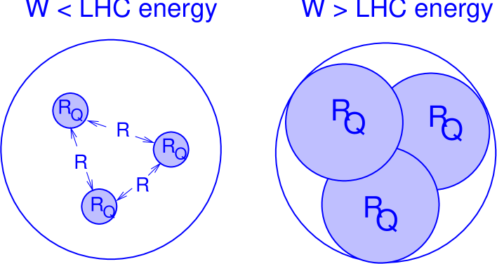
Figure 1: The proton structure at different energies in CQM.

In this paper we are going to develop a systematic approach to high energy scattering in CQM. To our surprise we found that only the simplest diagrams of this model has been discussed in details, namely the diagrams which include only interaction between a pair of quarks. In our model we include all possible quark interactions, considering an eikonal approximation for the scattering amplitude of two colliding quarks, (see Fig. (2)). In this case, the first contribution to the elastic amplitude will be simply nine interactions between constituent quarks in the protons. Further contributions to the amplitude will include the other interaction between quarks (see Fig. (3)). Taking into account all possible configurations of quarks we will obtain amplitude which contains nine different contributions with the alternating signs. Such a structure of the answer is similar to the scattering amplitude of light nuclei (tritium-tritium scattering). We will show, that the result satisfies the unitarity constraint, when we consider interactions between different configurations of the constituent quarks. The effects of interaction of several pairs of quarks is especially important at high energies. If we will consider our amplitude at asymptotically very high energy, where we will may replace eikonalized amplitude by a step function, the different parts of the amplitude will cancel each other and only the last diagram, in which all quarks of the projectile interact with all quarks of the target, will survive. This last diagram will give unitarized Froussart-like answer. In our estimates it turns out, that already at energies $\,\sqrt{s}\,=1855\,\,GeV\,\,$ we need to consider the interaction of the five pairs of quarks in the protons. At the LHC energies, the interaction of the seven quark pairs is essential. This structure of the interaction changes not only the high energy dependence of the scattering amplitude but also leads to a quite different impact parameter dependence of the answer. In the case of these multi-Pomeron exchanges between the different pairs of quarks, the amplitude has a minimum at low $b$. Such change is very important since it could affect the behavior of the slope both as function of energy and as function of momentum transfer.

Another interesting problem, addressed in this paper, is the values of parameters of the ”initial” Pomeron. Indeed, it is widely believed, that the ”soft” Pomeron is originated by the non-perturbative QCD contributions, which are out of theoretical control at the moment. Everything that we know about ‘soft” Pomeron is a mixture of our phenomenological knowledge with the general theoretical ideas on the properties of non-perturbative QCD contributions (see Refs. [8, 9, 10, 11, 12, 13, 14, 15, 16, 17, 18, 19]). The question is the following, can we obtain the well known phenomenological Pomeron using as ”initial” the Pomeron with the large intercept and small slope, i.e so called ”hard” Pomeron, [20] ? Does the ”hard” Pomeron play any role in the ”soft” interactions? There exist two different points of view on this question. The first one is that we need to introduce separately two objects, ”soft” and ”hard” Pomerons, which have different properties and contribute differently, each in a different kinematic region, see for example [8, 9, 12, 15] and references therein. Another point of view, see for example [21], is that non-perturbative physics comes in our calculations only in the form of the boundary and/or initial conditions and the ”soft” Pomeron arises as a result of unitarization effects and self-interactions of the ”hard” Pomerons in the amplitude. Our model may help to clarify the situation. Taking into account all effects of the unitarization, eikonalization and accounting all interactions between the different configurations of quarks, we will fit the experimental data. The fit will determine the parameters of the ”initial” Pomeron , such as its intercept and slope, as well as the radius of the constituent quark. We show in this paper, that the parameters of the initial ”soft” Pomeron are close to the parameters of the ”hard” Pomeron and quite different from the parameters of the Donnachie-Landshoff Pomeron [22], which is usually considered as a typical ”soft” Pomeron.

The structure of the paper is as follows. In Section 2 we discuss in more details our approach and methods of the calculations. In Section 3 we apply our model to the p-p data and fit the experimental data in order to find numerical values of the parameters of the ”initial” Pomeron. Section 4 is dedicated to the elastic amplitude as a function of the impact parameter. In this section we also consider the different contributions to the elastic amplitude due to interactions of different numbers of quark-quark pairs. In Section 5 we calculate the survival probability (SP) of the exclusive hard processes in p-p scattering . The cross section of the diffractive dissociation process is calculated in the Section 6. The last section, Conclusion, contains the main results of the paper as well as the discussion of a future work in the proposed direction.

2 Proton-proton scattering in the Pomeron approach

The key ingredient of the CQM is the quark-quark scattering amplitude. Considering this model, we need to determine the form of the single Pomeron exchange between two quarks. The next step will be the eikonalization of the single scattering amplitude, that means a replacement of the single Pomeron exchange in the scattering of the particular pair of quarks by the eikonal amplitude. The third step in our calculation will be the consideration of the interactions between all possible quark configurations in colliding protons, see Fig. 3. For this last step we need to know the wave function of the quarks in the proton and the vertices of the Pomerons-quarks interactions. Only after the determination of the wave function and vertices we will be able to calculate the diagrams for the quark-quark interactions.

Now let us consider these problems step by step.

2.1 Quark-quark interactions

We determine the amplitude for q-q and p-p scattering in the impact parameter representation. In this case the ”soft” Pomeron exchange for the interaction of the pair of the quarks (Pomeron propagator) has the following form (see more about soft Pomeron in Ref.[13, 22, 23]:

$$\Omega_{q-q}(Y,b)\,=\,\sigma_{0}\,e^{\Delta\,Y}\,\frac{e^{-b^{2}/R^{2}}}{\pi\,R^{2}}\,,$$ (1)

here, $\,Y=\ln\,(s/1\,GeV^{2})\,$ is the rapidity of the process, b is the impact parameter of the process, $\,\Delta\,$ is the intercept of the ’initial’, input Pomeron and

$$R^{2}=8\,R^{2}_{Q}\,+\,4\,\alpha^{{}^{\prime}}_{P}\,\ln\,(s/s_{0})\,\,.$$ (2)

Here $\,R^{2}_{Q}\,$ is the squared radius of the constituent quark and $\,\alpha^{{}^{\prime}}_{P}\,$ is the slope of the input Pomeron trajectory. The numerical values of the $\,\sigma_{0}\,$, $\,\Delta\,$, $\,R^{2}_{q}\,$ and $\,\alpha^{{}^{\prime}}_{P}\,$ we will find fitting data for p-p scattering. The eikonal amplitude, which is a ”main” ingredient in our calculations, we determine as follows:

$$P_{q-q}(Y,b)\,=\,1\,-\,e^{-\Omega_{q-q}(Y,b)\,/\,2}\,\,,$$ (3)

see Fig. 2, where $P_{q-q}$ is the imaginary part of the quark-quark scattering amplitude at high energy. Below , discussing the single quark-quark interaction amplitude, we will mean only the amplitude given by Eq. (3). The Pomeron of Eq. (1) we will consider only as the ”input”, initial Pomeron of our problem.

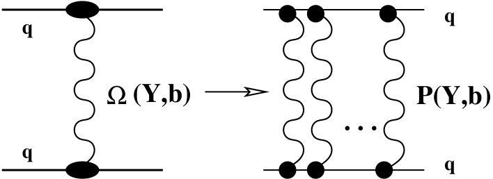
Figure 2: The Pomeron exchange and eikonalized quark-quark amplitudes.

Figure 3: The three first orders of the p-p elastic amplitude in the CQM.

2.2 The model of the proton

In order to take into account all possible configurations of the interacting pairs of the quarks, see Fig. 3 and all figures in the Appendices, we need to know the analytical expressions for the vertices of the quark-Pomeron interactions. It is clear, that we need to calculate only three types of such vertices, see Fig. 4-Fig. 6, where there are one, two or three groups of the Pomerons attached to the one, two or three quarks. In order to calculate these vertices we need to know the wave functions of the constituent quarks inside a proton. We use a very simple Gaussian model for this wave function, which corresponds to the oscillatory potential between pair of quarks in a proton. In this model we have ( see [24]):

$$\Psi\,=\,\frac{\alpha}{\pi\,\sqrt{3}}\,e^{-\frac{\alpha}{2}\left(\,\sum\,x^{2}_{i}\,\right)}\,$$ (4)

where the constant $\,\alpha\,$ is related to the electromagnetic radius of the proton:

$$\alpha\,=\,1/R^{2}_{electr}\,\approx\,0.06\,GeV^{2}\,\,.$$ (5)

For the diagram of Fig. 4, we have:

$$V_{1}(q)\,=\,\int\,|\Psi(x_{1},x_{2},x_{3})|^{2}\,\delta(\vec{x}_{1}+\vec{x}_{2}+\vec{x}_{3})\,e^{i\,\vec{q}\,\vec{x}_{1}}\,=\,e^{-\frac{q^{2}}{6\,\alpha}}\,.$$ (6)

Figure 4: The one Pomeron vertex in quark-quark interaction.

We determine the impact factor for two groups of Pomerons attached to two different quarks (see Fig. 5) :

$$V_{2}(q_{1},q_{2})\,=\,\int\,|\Psi(x_{1},x_{2},x_{3})|^{2}\,\delta(\vec{x}_{1}+\vec{x}_{2}+\vec{x}_{3})\,e^{i\,\vec{q}_{1}\,\vec{x}_{1}\,+\,\vec{q}_{2}\,\vec{x}_{2}\,}\,=\,e^{-\frac{q_{1}^{2}}{6\,\alpha}-\frac{q_{2}^{2}}{6\,\alpha}+\frac{\vec{q}_{1}\,\vec{q}_{2}}{6\,\alpha}}\,.$$ (7)

Figure 5: Two Pomeron vertex in quark-quark interaction.

The last impact factor is the vertex which is shown in Fig. 6. We have for this vertex :

$$V_{3}(q_{1},q_{2},q_{3})\,=\,\int\,|\Psi(x_{1},x_{2},x_{3})|^{2}\,\delta(\vec{x}_{1}+\vec{x}_{2}+\vec{x}_{3})\,e^{i\,\vec{q}_{1}\,\vec{x}_{1}\,+\,\vec{q}_{2}\,\vec{x}_{2}\,+\,\vec{q}_{3}\,\vec{x}_{3}\,}\,=\,e^{-\frac{(\vec{q}_{2}\,-\,\vec{q}_{3})^{2}}{8\,\alpha}-\frac{(\vec{q}_{1}-\vec{q}_{2}/2-\vec{q}_{3}/2)^{2}}{6\,\alpha}}\,.$$ (8)

In all three cases the total transferred momentum of the diagrams is defined as the sum of transverse momenta of all Pomerons ($q_{i}$): $\,k\,=\,\sum\,q_{i}\,$.

Figure 6: The three Pomeron vertex in q-q interaction.

2.3 The elastic amplitude of p-p scattering

We have all ingredients for the calculation of the elastic amplitude. In the CQM we can write the amplitude as the sum of the amplitudes with the different number of interacting quark pairs:

$$A(s,b)\,=\,A_{1pair}(s,b)-A_{2pairs}(s,b)+A_{3pairs}(s,b)+\,...\,+\,A_{9pairs}(s,b).$$ (9)

Here the amplitude for one quark pair interaction $A_{1pair}$ is equal to $P_{q-q}$ which is defined by Eq. (3). The maximum number of possible quark pair interactions in the amplitude is 9. The three first orders of the possible configurations of interactions are shown in Fig. 3 and the calculations of all other orders are presented in the Appendix B. The amplitude defined in a such way incorporates unitarity by construction. Indeed, checking the expressions for the different term of the amplitude, that are written in Appendix B, it is easy to see, that at asymptotically high energies only the last term of Eq. (9) will survive, giving the Froussart-like answer for the whole amplitude.

To calculate the contribution of the first diagram of Fig. 3, i.e. the first term of the r.h.s. of Eq. (9). we make Fourier transform of the vertex of Eq. (6) from momentum to impact parameter space:

$$\hat{V}_{1}(b)\,=\,\int\frac{d^{2}\,q}{4\,\pi^{2}}\,e^{-q^{2}/(6\alpha)+i\,\vec{q}\,\vec{b}}\,=\,\frac{3\,\alpha}{2\,\pi}e^{-\frac{3\alpha}{2}\,b^{2}}\,.$$ (10)

Using this vertex we obtain the contribution to the elastic amplitude from the one Pomeron exchange $\,A_{1q-q}(s,b)\,$, which is :

$$A_{1pair}(s,b)\,=9\,\frac{9\,\alpha^{2}}{4\,\pi^{2}}\int\,d^{2}\,b_{1}\,\int\,d^{2}\,b_{2}\,e^{-\frac{3\alpha\,}{2}(\vec{b}-\vec{b}_{1})^{2}}\,P_{q-q}(Y,b_{2})\,e^{-\frac{3\alpha}{2}\,(\vec{b}_{1}-\vec{b}_{2})^{2}}\,\,,$$ (11)

where the first coefficient in Eq. (11) is the total number of q-q interactions in this order. Using more complicated vertices, which are given by Eq. (7) and Eq. (8), we calculate all terms that contribute to the elastic amplitude, i.e. terms on the r.h.s. of Eq. (9). In Appendices A,B the resulting expressions for the amplitude $\,A(s,b)\,$ are written as well as the examples of the calculations of the diagrams with the different numbers of interacting pairs of quarks.

2.4 The total, elastic cross sections and the elastic slope $B_{el}$ of the proton-proton interaction

The expression for the amplitude (Appendix B), is determined in the impact parameter space and now we can easily calculate the different cross sections for the processes of interest.

$\mathbf{\sigma}_{\mathbf{tot}}$.     The total cross section in impact parameter representation is simply

$$\sigma_{tot}(s)\,=\,2\,\int\,d^{2}\,b\,Im\,A(s,b)\,.$$ (12)

Fitting the experimental data at low energies we also add to this cross section the contribution of the secondary Reggeons, $\,\sigma_{tot}^{Reg}\,$, see [25].

$\mathbf{\sigma}_{\mathbf{el}}$.     The elastic cross section in the same framework is equal:

$$\sigma_{el}(s)\,=\,\int\,d^{2}\,b\,|A(s,b)|^{2}\,\,=\,\,\int\,d^{2}\,b\,(\,Im\,A(s,b)\,)^{2}.$$ (13)

where we assumed that the quark-quark amplitude is mostly imaginary as it follows from the eikonal approximation.

$\mathbf{B}_{\mathbf{el}}$.    We consider only the first term of the elastic amplitude, i.e $\,A_{1q-q}(s,b)\,$. In this case we have for the slope $\,B_{el}\,$:

$$B_{el}\, = \,\,\frac{\frac{9\,\alpha^{2}}{4\,\pi^{2}}\,\int\,d^{2}\,b_{1}\,\int\,d^{2}\,b_{2}\,\int\,d^{2}\,b\,\,b^{2}\,\,e^{-\frac{3\alpha\,}{2}(\vec{b}-\vec{b}_{1})^{2}}\,P_{q-q}(Y,b_{2})\,e^{-\frac{3\alpha}{2}\,(\vec{b}_{1}-\vec{b}_{2})^{2}}\,}{2\,\int\,\,d^{2}\,b\,P_{q-q}(Y,b)}\,=\,$$ (14)

$$= \,\frac{1}{\alpha}\,\frac{\sigma_{tot}^{1q-q}}{\sigma_{tot}^{1q-q}}\,+\,\frac{\int\,\,d^{2}\,b\,\,b^{2}\,\,P_{q-q}(Y,b)}{\sigma_{tot}^{1q-q}}\,.$$ (15)

Here

$$\sigma_{tot}^{1q-q}\,=\,2\,\int\,d^{2}\,b\,P_{q-q}(Y,b)\,.$$

We add the contribution of the secondary Reggeons to this expression , which is needed to be taken into account at low energies:

$$B_{el}\,=\,\frac{9\,\sigma_{tot}^{1q-q}}{9\,\sigma_{tot}^{1q-q}+\sigma_{tot}^{Reg}}\,R_{electr}^{2}\,+\,\frac{9\,\int\,\,d^{2}\,b\,\,b^{2}\,\,P_{q-q}(Y,b)}{9\,\sigma_{tot}^{1q-q}+\sigma_{tot}^{Reg}}\,+\,2\,(\alpha^{{}^{\prime}}_{R}-\alpha^{{}^{\prime}}_{SP})\,\ln\,(s/s_{0})\,\frac{\sigma_{tot}^{Reg}}{9\,\sigma_{tot}^{1q-q}+\sigma_{tot}^{Reg}}\,.$$ (16)

The third term of the r.h.s of Eq. (16) contains the contribution of the secondary Reggeons, which we do not consider in our model. The secondary Reggeons we account only on the level of proton-proton scattering. Therefore, the parameters which we take for this contribution have a pure phenomenological origin. We take for the slope of secondary Reggeons $\,\alpha^{{}^{\prime}}_{R}\,=\,0.86\,GeV^{-2}\,$ and for the slope of phenomenological ”soft” Pomeron $\,\alpha^{{}^{\prime}}_{SP}\,=\,0.25\,GeV^{-2}\,$ at $\,\sqrt{s}_{0}\,=\,9\,GeV\,$ in the r.h.s of Eq. (16), see [22, 23, 25]. Generalizing this expression to the case of full elastic amplitude ( see Eq. (9)) we obtain at low energies:

$$B_{el}\, = \,\frac{9\,\sigma_{tot}^{1q-q}}{\sigma_{tot}+\sigma_{tot}^{Reg}}\,R_{electr}^{2}\,+\,\frac{9\,\int\,\,d^{2}\,b\,\,b^{2}\,\,P_{q-q}(Y,b)}{\sigma_{tot}+\sigma_{tot}^{Reg}}\,+\,$$ (17)

$$+ \,2\,(\alpha^{{}^{\prime}}_{R}-\alpha^{{}^{\prime}}_{SP})\,\ln\,(s/s_{0})\,\frac{\sigma_{tot}^{Reg}}{\sigma_{tot}+\sigma_{tot}^{Reg}}\,+\,\sum_{i=2}^{9}\frac{\int\,d^{2}\,b\,\,b^{2}\,\,Im\,A_{i}(b,s)}{\sigma_{tot}+\sigma_{tot}^{Reg}}\,,$$ (18)

whereas at high energy we have

$$B_{el}\,=\,\frac{9\,\sigma_{tot}^{1q-q}}{\sigma_{tot}}\,R_{electr}^{2}\,+\,\frac{9\,\int\,\,d^{2}\,b\,\,b^{2}\,\,P_{q-q}(Y,b)}{\sigma_{tot}}\,+\,\sum_{i=2}^{9}\frac{\int\,d^{2}\,b\,\,b^{2}\,\,Im\,A_{i}(b,s)}{\sigma_{tot}}\,.$$ (19)

It is also interesting to calculate the elastic cross section using simple expression for the elastic cross section which is obtained in the model with the phenomenological ”soft” Pomeron. Indeed, in this case we calculate the elastic cross section using the following formula:

$$\sigma_{el}(s)\,=\,\frac{\sigma_{tot}^{2}}{16\,\pi\,B_{el}}\,.$$ (20)

This expression is correct only in the case when one ”soft” Pomeron is considered. It will be interesting to compare the calculations of elastic cross section given by Eq. (13) with the calculations of Eq. (20). Indeed, in this case we check the possibility to reproduce the simple result of Eq. (20) by the theory where many eikonalized Pomeron exchanges are taken into account. So, in the next section we will perform the data fitting and will make the calculations using both expressions, Eq. (13) and Eq. (20) in order to show the importance of many quark pairs interaction.

3 The proton-proton scattering data and the parameters of the input Pomeron

Now, we are able to apply our model to the p-p interactions and, fitting the experimental observables, we will extract the values of the parameters of our input Pomeron ( see Eq. (1)). In Fig. 7 we present the plots for the total cross section, elastic cross section and elastic slope in $\,W=23-1855\,\,GeV\,$ energy range. We perform all calculations numerically using the formulae of the previous subsection with the amplitude written in the Appendix B. There are two different plots which we present for elastic cross section using definitions Eq. (13) and Eq. (20). The solid line represents the elastic cross section given by Eq. (20) and dashed line represents calculations performed with Eq. (13).

Fig. (7)-a	Fig. (7)-b
Fig. (7)-c

Figure 7: The plots for the total cross section, Fig. (7)-a, elastic cross section , Fig. (7)-c, and elastic slope, Fig. (7)-b. The experimental data are from [25] and references therein.

Fig. (8)-a	Fig. (8)-b
Fig. (8)-c

Figure 8: The plots for the total cross section, Fig. (8)-a, elastic cross section , Fig. (8)-c, and elastic slope, Fig. (8)-b, at high energies.

From these plots we see, that the model describes the experimental data quite well. The parameters of the single Pomeron of Eq. (1) extracted from the data fitting are the following:

• the slope of the input Pomeron trajectory:

  $$\alpha^{{}^{\prime}}\,=\,0.08\,GeV^{-2};$$ (21)

• input Pomeron’s intercept:

  $$\Delta\,=\,0.118\,;$$ (22)

• the value of cross section for the input Pomeron at $s_{0}=1\,\,GeV^{2}$ :

  $$\sigma_{0}\,=\,6.3\,GeV^{-2}\,;$$ (23)

• the radius of the constituent quark:

  $$R^{2}_{quark}\,=\,0.16\,\,GeV^{-2}.$$ (24)

With these parameters we extrapolate our calculations for the cross sections and slope at higher energies. The resulting plots are shown in Fig. 8.

It should be stressed that the above parameters are quite different from the Donnachie-Landshoff Pomeron [22]. The Pomeron intercept, which we obtained, is higher and the slope is much lower than the intercept and slope of the D-L Pomeron. We may conclude, that such small value of the Pomeron slope indicates that our input Pomeron can have a ”hard” origin.

4 Behavior of the elastic amplitude of p-p scattering in our model

The elastic amplitude in our model has a sufficiently complex structure. It contains contributions from different configurations for the interactions of quarks inside the protons. We found all possible terms which contribute to the elastic amplitude, see Appendix B, and, therefore, we can find out which terms in elastic amplitude are important at different energies. It turns out, that even at low energies the two quark pairs interactions, i.e. interactions between two quarks in one proton with two quarks in another proton, are not negligible. At Tevatron energy, $\,\sqrt{s}\,=\,1855\,GeV\,$, we already need to take into account the contributions from the five pairs of interacting quarks. At energy of order of the LHC energy, $\,\sqrt{s}\,=\,15000\,GeV\,$, the contribution of the interaction of the seven quark pairs is valuable. At this energy the contribution of two quark pair interaction exceeds the contribution of one quark pair interaction, see Fig. 9. This is a signal that the parton clouds start to overlap, leading to the picture of Fig. (1).

Fig. (9)-a	Fig. (9)-b
Fig. (9)-c

Figure 9: The contributions to the elastic amplitude from the interactions of different numbers of quark pairs at different energies.

From Fig. 9 we also see, that even at $\,\sqrt{s}\,=\,1855\,GeV\,$ energy, the one quark pair contribution to the elastic amplitude exceeds unity . The unitarization of the amplitude in this case is achieved not by eikonalization of the quark-quark interaction but by including more complicated configurations of the quarks inside of the protons in the elastic amplitude. Therefore, the form of impact parameter dependence of the amplitude turns out to be different from the usual Gaussian one. Indeed, the contribution of two quark pair interactions, which have a negative sign in the amplitude is equal or larger than contribution of one quark pair interaction. At the same time the one quark pair interaction is wider in the impact parameter space, see again Fig. 9. The contributions of all terms in the elastic amplitude lead, therefore, to the situation where the maximum of the elastic amplitude moves from the zero impact parameter to the impact parameter $\,b\,\approx\,2\,GeV^{-1}\,$, see Fig. 10. This effect reflects very simple physics. At high energy at small impact parameter the multi quark pair interactions are important and elastic production becomes mostly peripheral.

Figure 10: The elastic amplitude of the p-p scattering as function of impact parameter at different energies.

5 Survival probability (SP) of the ’hard’ processes in p-p scattering

In this section we consider the calculation of the survival probability for the process:$p+p\to p+[LRG]+dijet+[LRG]+p$, where $p$ and $p$ are the colliding protons and LRG is the large rapidity gap. In this process there are two large rapidity gaps – the intervals of rapidity without secondary hadrons. The cross sections of such processes are small in comparison with the inclusive production or in other word, in comparison with the process where no rapidity gap is selected. The ratio of these two processes, exclusive and inclusive (or the process without LRG), we call survival probability of large rapidity gap (see Ref.[26]). In the simple case of the eikonal approach to proton-proton interaction, the survival probability is determined by a simple formula (see Ref.[26, 27]):

$$\hat{S}^{2}\,=\,\frac{\int\,d^{2}\,b\,A(s,b)\,\sigma_{hard}(b)}{\int\,d^{2}\,b\,\,\sigma_{hard}(b)\,}\,$$ (25)

where

$$\,A(s,b)\,=\,e^{-\Omega(s,b)}\,$$ (26)

is the probability that no inelastic interaction between the scattered hadrons has happened at energy $\,\sqrt{s}\,$ and impact parameter $\,b\,$.

Using a simple Gaussian parameterization for $\sigma_{hard}(b)$ , namely,

$$\sigma_{hard}(b)\,=\,\sigma_{hard}\,\frac{e^{-\frac{b^{2}}{R^{2}_{H}}}}{4\pi\,R^{2}_{H}}\,,$$ (27)

with

$$R^{2}_{H}\,\,=\,\,8\,GeV^{-2}$$ (28)

we reduce Eq. (25) to the form

$$\hat{S}^{2}\,=\,\frac{1}{\pi\,R^{2}_{H}}\,\int\,d^{2}\,b\,A(s,b)\,e^{-\frac{b^{2}}{R^{2}_{H}}}\,\,.$$ (29)

The difference of the calculation of the SP in our model from the calculations above is that we consider as principle degrees of freedom the constituent quarks but not protons. Therefore, we need to determine the expression for SP in terms of the interacting quark pairs. We begin with the discussion of the cross section for the exclusive ”hard” production in the case of interaction of only one pair of quarks. For this process we have:

$$\sigma_{hard}(b)\,=\,\sigma_{hard}\,\left(\,\hat{A}_{1pair}(s,b)\right)^{2}\,,$$ (30)

with the amplitude $\hat{A}_{1pair}(s,b)$, calculated from Eq. (11) with he following replacement

$$P_{q-q}(Y,b_{2})\,\rightarrow\,\frac{e^{-\frac{b_{2}^{2}}{2\,R^{2}_{Q-H}}}}{2\pi\,R^{2}_{H}}\hat{P}_{q-q}(Y,b_{2})\,,$$ (31)

where

$$\hat{P}_{q-q}(Y,b_{2})\,=\,1\,-\,P_{q-q}(Y,b_{2})\,=\,e^{-\Omega_{q-q}(Y,b_{2})/2}\,$$ (32)

in Eq. (31) means that t no inelastic interactions occur between the considered pair of quarks. This pair of quarks, which produces ”hard” jet, interacts elastically. The amplitude of this process is illustrated in Fig. 11.

Figure 11: The first order amplitude of the LRG ”hard” process.

In expression for the $\hat{A}(s,b)$, we need to introduce a new ”hard” radius $\,R^{2}_{Q-H}\,$, which related to the ”hard” process on the quark level. The numerical value of $\,R^{2}_{Q-H}\,$ we find in the following way. For simplest process of ”hard” production without any ”soft” rescattering, the answer will be the same for any model :

$$e^{-\frac{b^{2}}{2\,R^{2}_{H}}}\,=\,\,9\,\frac{9\,\alpha^{2}}{4\,\pi^{2}}\,\int\,d^{2}\,b_{1}\,\int\,d^{2}\,b_{2}\,e^{-\frac{3\alpha\,}{2}(\vec{b}-\vec{b}_{1})^{2}}\,\,e^{-\frac{b_{2}^{2}}{2R^{2}_{Q-H}}}\,e^{-\frac{3\alpha}{2}\,(\vec{b}_{1}-\vec{b}_{2})^{2}}\,.$$ (33)

Indeed, we can see, that using this equality in Eq. (30), we reproduce the expression given by Eq. (27). From the Eq. (33), we obtain the value of $\,R^{2}_{Q-H}\,$:

$$R^{2}_{Q-H}\,\approx\,1.1\,\,GeV^{-2}\,\,.$$ (34)

Generalizing the procedure given by Eq. (31) we obtain the answer for SP amplitude $\hat{A}(s,b)$ in the all orders. Indeed, any term of the amplitude given in Appendix B, see Eq. (B.1), have the integration over the product of the eikonalized amplitudes of the interacting quark pairs $\,P_{q-q}(b_{i})\,...\,P_{q-q}(b_{j})\,$. When we calculate the SP, we should take into account the possibility that the ”hard” process can occur in the interaction of any pair of quarks. Therefore, for the pair with the ”hard” process the replacement of Eq. (31) should be performed, whereas other pairs of quarks will still interact elastically. It means, that for any integral in expansion of Eq. (B.1) of elastic amplitude, we will make the following replacement for any term of $\,P_{q-q}(b_{i})\,...\,P_{q-q}(b_{j})\,$ - type :

$$P_{q-q}(b_{i})\,...\,P_{q-q}(b_{j})\,\rightarrow\,\frac{e^{-\frac{b_{i}^{2}}{2\,R^{2}_{Q-H}}}}{2\pi\,R^{2}_{H}}\hat{P}_{q-q}(b_{i})\,...\,P_{q-q}(b_{j})\,$$ (35)

for each $\,P_{q-q}(b_{k})\,$ in the chain $\,P_{q-q}(b_{i})\,...\,P_{q-q}(b_{j})\,$. This procedure is illustrated by Fig. 12 for the case of the interaction of two pairs of quarks.

Figure 12: The general structure of the amplitude of the LRG ”hard” process for the case of interaction of two quark pairs.

Performing these replacements and summing all terms, we obtain a new amplitude $\,\hat{A}(s,b)\,$ ( see Eq. (B.1)). In Appendix C we show the example of this procedure for the $\,A_{3pairs}(s,b)\,$ term of the elastic amplitude $\,A(s,b)\,$. With this amplitude, $\,\hat{A}(s,b)\,$, we determine the ”hard” cross section as follows:

$$\sigma_{hard}\,\propto\,\int\,d^{2}\,b\,\left(\,\hat{A}(s,b)\right)^{2}\,,$$ (36)

where the first term of this expansion has the form:

$$\sigma_{hard}^{1}\,\propto\,\frac{81}{4\,\pi^{2}\,R^{4}_{H}}\int\,d^{2}\,b\,\left(\,\frac{9\,\alpha^{2}}{4\,\pi^{2}}\int\,d^{2}\,b_{1}\,\int\,d^{2}\,b_{2}\,e^{-\frac{3\alpha\,}{2}(\vec{b}-\vec{b}_{1})^{2}}\,\hat{P}_{q-q}(Y,b_{2})\,e^{-\frac{b_{2}^{2}}{2R^{2}_{Q-H}}}\,e^{-\frac{3\alpha}{2}\,(\vec{b}_{1}-\vec{b}_{2})^{2}}\,\right)^{2}$$ (37)

Finally, the answer for the survival probability factor in all orders of the expansion of Eq. (B.1) looks as follows:

$$\hat{S}^{2}\,=\,4\,\pi^{2}\,R^{4}_{H}\,\frac{\int\,d^{2}\,b\,\left(\,\hat{A}(s,b)\right)^{2}\,}{\int\,d^{2}\,b\,\left(\,9\,\,\frac{9\,\alpha^{2}}{4\,\pi^{2}}\int\,d^{2}\,b_{1}\,\int\,d^{2}\,b_{2}\,e^{-\frac{3\alpha\,}{2}(\vec{b}-\vec{b}_{1})^{2}}\,\,e^{-\frac{b_{2}^{2}}{2R^{2}_{Q-H}}}\,e^{-\frac{3\alpha}{2}\,(\vec{b}_{1}-\vec{b}_{2})^{2}}\,\right)^{2}}\,.$$ (38)

For example, there is the first term, which contributes to the $\,\hat{S}^{2}\,$:

$$\hat{S}_{1}^{2}\,=\,\frac{\int\,d^{2}\,b\,\left(\,\,\frac{9\,\alpha^{2}}{4\,\pi^{2}}\int\,d^{2}\,b_{1}\,\int\,d^{2}\,b_{2}\,e^{-\frac{3\alpha\,}{2}(\vec{b}-\vec{b}_{1})^{2}}\,\,e^{-\frac{b_{2}^{2}}{2R^{2}_{Q-H}}}\,\hat{P}_{q-q}(Y,b_{2})\,e^{-\frac{3\alpha}{2}\,(\vec{b}_{1}-\vec{b}_{2})^{2}}\,\right)^{2}\,}{\int\,d^{2}\,b\,\left(\,\frac{9\,\alpha^{2}}{4\,\pi^{2}}\int\,d^{2}\,b_{1}\,\int\,d^{2}\,b_{2}\,e^{-\frac{3\alpha\,}{2}(\vec{b}-\vec{b}_{1})^{2}}\,\,e^{-\frac{b_{2}^{2}}{2R^{2}_{Q-H}}}\,e^{-\frac{3\alpha}{2}\,(\vec{b}_{1}-\vec{b}_{2})^{2}}\,\right)^{2}}\,.$$ (39)

The values of the survival probability factor, $\,\hat{S}^{2}\,$, calculated in this approach, are shown in the Table 1.

$SP\,(\,\sqrt{s}=23\,GeV)$	$SP\,(\,\sqrt{s}=1855\,GeV$	$SP\,(\,\sqrt{s}=15000\,GeV)$	$SP\,(\,\sqrt{s}=18000\,GeV)$
0.23	0.052	0.0175	0.0155

Table 1: The survival probability factor as a function of $\sqrt{s}$

We see, that these values are close to the values of survival probability for the central diffraction process calculated in Ref. [28].

Fig. (13)-a	Fig. (13)-b

Figure 13: The impact parameter behavior of the integrant in the numerator of Eq. (38) at energies $\,W=1855\,\,GeV\,$ and $\,W=18000\,\,GeV\,$.

We also performed the calculation of the integrant in the numerator of Eq. (38) , which is proportional to the amplitude of the ”hard” central diffraction process. The plots of this integrant as a function of impact parameter at different energies are presented in Fig. 13. Considering these graphs we conclude, that the main contribution to the amplitude of the central diffraction ”hard” production comes from the non-central values of impact parameter and it is almost zero for the central impact parameter at high energies.

6 The cross section of the diffraction dissociation

The elastic amplitude of the considered model accounts many Pomeron exchanges between different pairs of quarks. Now, we want to calculate the cross section of the diffraction dissociation processes taking into account all these processes. The diffractive dissociation (DD) processes for us are all processes where no particle have been produced in the rapidity region between two scattered protons. From the unitarity constraint we have:

$$\sigma_{tot}\,=\,\sigma_{el}\,+\,\sigma_{inel}\,+\,\sigma_{DD}\,.$$ (40)

Therefore:

$$\,\sigma_{DD}\,=\,\sigma_{tot}\,-\,\sigma_{el}\,-\,\sigma_{inel}.$$ (41)

From our previous calculations we know the values of $\,\sigma_{el}\,$ and $\,\sigma_{tot}\,$. So, in order to calculate $\,\sigma_{DD}\,$ we need to calculate the value of $\,\sigma_{inel}\,$. The calculation of $\,\sigma_{inel}\,$ is pretty simple. In the first order, where

$$\sigma_{total}^{1}\,=\,2\,\int\,d^{2}\,b\,A_{1pair}(s,b)\,=\,18\,\int\,d^{2}\,b\,P_{q-q}(Y,b)\,,$$ (42)

for $\,\sigma_{inel}\,$ we have:

$$\sigma_{inel}\,=\,\int\,d^{2}\,b\,A_{1pair}^{inel}(s,b)\,=\,9\,\int\,d^{2}\,b\,P_{q-q}^{inel}(Y,b)\,,$$ (43)

with

$$P^{inel}_{q-q}(Y,b)\,=\,1\,-\,e^{-\Omega_{q-q}(Y,b)}\,.$$ (44)

The calculation of $\,\sigma_{inel}\,$ for all possible interactions between the pairs of the quarks in the protons we perform using the following simple receipt. In each expression for $\,\sigma_{tot}\,$

$$\sigma_{total}\,=\,2\,\int\,d^{2}\,b\,A(s,b)\,,$$ (45)

we make replacement:

$$P_{q-q}(Y,b_{i})...P_{q-q}(Y,b_{j})\,\rightarrow\,\frac{1}{2}\,P_{q-q}^{inel}(Y,b_{i})...P_{q-q}^{inel}(Y,b_{j})\,,$$ (46)

with the $\,P_{q-q}^{inel}\,$ given by Eq. (44). After the calculations of $\,\sigma_{inel}\,$ with the help of Eq. (43) we obtain the value of $\,\sigma_{DD}\,$. The result of calculations for the energy range $\,W\,=\,100\,-\,3000\,\,\,GeV\,$ is shown in Fig. 14, as well as the sum of elastic and inelastic cross sections in comparison with the total cross section.

Fig. (14)-a	Fig. (14)-b

Figure 14: The sum of elastic and inelastic cross sections in comparison with the total cross section and DD cross section as the function of $W\,=\,\sqrt{s}$.

For the energies higher than $\,W\,=\,3000\,\,GeV\,\,$, the cross section of diffractive dissociation process is almost zero, see Table 2, as it must be at high energies when we approach the ”black disc” limit. Nevertheless, it is important to notice, that in calculations of DD processes, we neglected the diffraction dissociation processes with the large mass production. Such processes may be described if we introduce in the model the triple Pomeron vertex, see [6]. We did not consider this vertex in our calculations, therefore, our result for the cross section of the DD processes, which is the sum of single diffraction and double diffraction processes, is smaller than it could be in the case when the triple Pomeron vertex is included.

$\sigma_{DD}(\sqrt{s}=7000\,GeV)$	$\sigma_{DD}(\sqrt{s}=10000\,GeV)$	$\sigma_{DD}(\sqrt{s}=15000\,GeV)$	$\sigma_{DD}(\sqrt{s}=18000\,GeV)$
2.3  mb	0.4  mb	0.35  mb	0.3  mb

Table 2: The diffractive dissociation cross section at high energies as a function of $\sqrt{s}$.

7 Conclusion

In this paper we consider the proton-proton interactions in the framework of the Constituent Quark Model (CQM) at high energies. The typical ”soft” process of p-p scattering we described taking into account all interactions between pairs of the quarks in the protons, modeling the quark-quark interaction by eikonal formula. It turns out , that in this model the interactions of one, two or three quarks from one proton with two or three quarks from the second proton surprisingly become essential even at low energies. Indeed, if we look at Fig. 9, we see, that even at energy $\,\sqrt{s}\,=23\,GeV\,$ the contribution from the interaction of two pairs of quarks is approximately one third from the contribution of one pair. Of course, at higher energies the contributions of more interacting quark pairs became to be more important. For example, at LHC energy the interactions of one and two pairs of quarks equally contribute to the elastic amplitude and at this energy we need to account the contribution of seven quark pairs. This interaction picture leads to the very natural scenario of the unitarization. At high energies the contributions from the interaction of one and two pairs of quarks cancel each other, and final amplitude at given impact parameter is smaller than one, see Fig. 10. We see, that in this case the unitarization is achieved by exploring internal structure of the proton rather than details of interactions. However, we should stress, that we assume that the quark-quark interactions is described by the eikonal approach. This specific mechanism manifests itself in the form of the b-dependence of the amplitude, which is quite different from the usual $\,b\,$ dependence. Our amplitude has maximum at $\,b\,\approx\,2\,GeV^{-1}\,$ at high energy, that means that elastic production is mostly peripheral at high energies.

Another result , observed in the present model and related to the unitarization of the amplitude, is the relatively small value of the amplitude at zero impact parameter. Indeed, even at energy $\,\sqrt{s}\,=18000\,GeV\,$ at $\,b\,=\,0\,$ the amplitude is not close to one. The interactions are still ”grey” and not ”black”. Many Pomeron interactions between different quark configurations in both protons lead to the ”grey ” picture in spite of the large contributions of the one, two or three interacting quark pairs.

The considered model fits the experimental data pretty well, see Fig. 7. Using the parameters of the ”input” Pomeron , which we obtained through the data fitting, we can predict the values of the cross sections at high energies. Doing so, we did not find the deviation of the behavior of the elastic slope, $\,B_{el}\,$, from the simple linear parameterization, see plot of Fig. 8. The explanation of this effect is the following. In spite of the hope, that the constituent quarks will have strong overlapping at high energies and this effect will change the energy behavior of the $\,B_{el}\,$, it actually does not happen. The value of the size of constituent quark obtained from the data fit is small, $\,R^{2}_{quark}\,\approx\,0.16\,GeV^{-2}\,\,$. The slope of the initial quark-quark amplitude, which is our ”input” Pomeron, also turns out to be small , $\alpha^{{}^{\prime}}\,\approx\,0.08\,GeV^{-2}\,$. Therefore, even at energy $\,\sqrt{s}\,=18000\,GeV\,$ we obtain for the radius of the constituent quark $\,R_{quark}\,\approx\,0.3\,-\,0.4\,fm\,\,$, that is still in two times smaller than the radius of the proton. This again supports the conclusion, that our interactions at LHC energy still far from the ”black” disk limit.

We also calculated the survival probability factor for different energies and it turns out to be similar to the values obtained in model proposed in Ref. [28]. The parameters of the ”input” Pomeron in our paper and in Ref. [28] are close, in spite of the fact that we did not involve any non-perturbative physics in our calculations. The intercept of the ”input” Pomeron, which we obtained , is $\,\Delta\,\approx\,0.12\,$ . This intercept is larger than the intercept of the paper [28]. The slope, $\alpha^{{}^{\prime}}\,\approx\,0.08\,GeV^{-2}\,$, is very close to the one of the paper [28]. Considering the impact parameter dependence of the amplitude of the exclusive central diffraction ”hard” process, see Fig. 13, we see, that the maximum of the amplitude locates at peripheral impact parameter, $\,b\,\approx\,3\,GeV^{-2}\,$ at energy of LHC. The probability of this process at zero impact parameter is almost zero.

The values of the parameters of our ”input” Pomeron, the slope ($\alpha^{{}^{\prime}}_{P}\,\approx\,0.08GeV^{-2}$ and the intercept $\Delta\approx\,0.2$, give rise to the idea that this Pomeron is not ”soft” (see Ref. [23] for the typical parameters of the soft Pomeron). The parameters that we obtained related to so called ”hard” Pomeron. Therefore, the one of the result of this paper is the idea that, perhaps, we do not need to introduce ”soft” Pomeron in order to describe the ”soft” data. Considering the internal structure of the colliding hadrons as well as the unitarization corrections for the amplitude we can describe p-p data using only one, ”hard” Pomeron.

Appendix A:

In this appendix, as an example of our calculations, we calculate two diagrams, which contribute to the elastic amplitude: the first diagram of Fig. 15 and the first diagram of Fig. 16.

Figure 15: Four diagrams of the three quark pair interaction. The wave line describes the eikonal amplitude for quark-quark interaction $P(Y,b)$.

We begin with the first diagram of Fig. 15. There are six diagrams of this type and we need two vertices (see Eq. (6) and Eq. (8)) for the calculations:

$$V_{up}(k)=e^{-k^{2}/(6\,\alpha)}\,,$$

and

$$V_{down}(k)=e^{-\frac{1}{8\,\alpha}(\vec{q}_{2}-\vec{q}_{3})^{2}-\frac{1}{6\,\alpha}(\vec{q}_{1}-\vec{q}_{2}/2-\vec{q}_{3}/2)^{2}\,}\,,$$

where $\,q_{i}\,$ is the momentum transferred of each single Pomeron, and $\,k\,\,=q_{1}+q_{2}+q_{3}\,$. So, we have for our diagram:

$$D_{1,3pairs}(k)\,=\,6\,\int\,\prod_{i=1}^{3}\,\frac{d^{2}\,q_{i}}{4\,\pi^{2}}\,P_{q-q}(q_{i})\,e^{-k^{2}/(6\,\alpha)}\,e^{-\frac{1}{8\,\alpha}(\vec{q}_{2}-\vec{q}_{3})^{2}-\frac{3}{8\,\alpha}(\vec{q}_{1}-\vec{k}/3)^{2}\,}\,(4\,\pi^{2}\,\delta^{2}(\vec{k}-\vec{q}_{1}-\vec{q}_{2}-\vec{q}_{3})\,)\,$$ (A.1)

where $\,P_{q-q}(q_{i})\,$ is the Fourier transform of amplitude given by Eq. (3).

Since we have no simple analytic expression for $\,P_{q-q}(q_{i})\,$, we make Fourier transform for each function $\,P_{q-q}(q_{i})\,$ and rewrite our expression in terms of $\,P_{q-q}(b_{i})\,$:

$$P_{q-q}(q_{i})\,=\,\int\,d^{2}\,b_{i}\,P_{q-q}(b_{i})\,e^{i\vec{q}_{i}\,\vec{b}_{i}}\,.$$ (A.2)

Here $\,b_{i}\,$ is the impact parameter variable, which is conjugated to momentum $\,q_{i}\,$ of the single Pomeron. We also make Fourier transform from $\,k\,$ to impact parameter variable $\,b\,$. We obtain:

$$D_{1,3pairs}(b)\, = \,\frac{6}{64\,\pi^{6}}\,\int\,\prod_{i=1}^{3}\,d^{2}\,b_{i}\,P_{q-q}(b_{i})\,\int\,\prod_{i=1}^{3}\,d^{2}\,q_{i}\,\,\int\,d^{2}\,k\,\,\,e^{-i\,\vec{k}\,\vec{b}}$$ (A.3)

$$\,e^{i\,\sum_{i=1}^{3}\,\vec{q}_{i}\,\vec{b}_{i}}\,e^{-k^{2}/(6\,\alpha)}\,e^{-\frac{1}{8\,\alpha}(\vec{q}_{2}-\vec{q}_{3})^{2}-\frac{3}{8\,\alpha}(\vec{q}_{1}-\vec{k}/3)^{2}\,}\,\,\delta^{2}(\vec{k}-\vec{q}_{1}-\vec{q}_{2}-\vec{q}_{3})\,.$$ (A.4)

To make this expression easier for calculations we introduce new variables:

$$x_{1}=q_{2}-q_{3}\,;\,\,x_{2}=q_{1}-k/3\,;\,\,x_{3}=q_{3}\,\,,\\$$ (A.5)

$$q_{1}=x_{2}+k/3\,;\,\,q_{2}=x_{1}+x_{3}\,;\,\,q_{3}=x_{3}\,\,.$$

The Jacobian of this transformations is equal to unity; and we obtain:

$$D_{1,3pairs}(b)\, = \,\frac{6}{64\,\pi^{6}}\,\int\,\prod_{i=1}^{3}\,d^{2}\,b_{i}\,P_{q-q}(b_{i})\,\int\,\prod_{i=1}^{3}\,d^{2}\,x_{i}\,\,\int\,d^{2}\,k\,\,\,e^{-i\,\vec{k}\,\vec{b}}\,e^{i\,\vec{b}_{1}\,(\vec{x}_{2}+\vec{k}/3)}\,$$ (A.6)

$$\,e^{i\,\vec{b}_{2}\,(\vec{x}_{3}+\vec{x}_{1})}\,e^{i\,\vec{b}_{3}\,\vec{x}_{3}}\,\,e^{-\frac{1}{6\,\alpha}\,k^{2}\,-\,\frac{1}{8\,\alpha}\,x_{1}^{2}\,-\,\frac{3}{8\,\alpha}\,x_{2}^{2}\,}\,\,\delta^{2}(2\vec{k}/3-\vec{x}_{1}-\vec{x}_{2}-2\vec{x}_{3})\,.$$ (A.7)

Performing the $\,x_{3}\,$ integration we have:

$$D_{1,3pairs}(b)\, = \,\frac{6}{4\,64\,\pi^{6}}\,\int\,\prod_{i=1}^{3}\,d^{2}\,b_{i}\,P_{q-q}(b_{i})\,\int\,\prod_{i=1}^{2}\,d^{2}\,x_{i}\,\,\int\,d^{2}\,k\,\,\,e^{i\,\vec{k}\,(-\vec{b}+\vec{b}_{1}/3+\vec{b}_{2}/3+\vec{b}_{3}/3)}\,$$ (A.8)

$$\,e^{i\,\vec{x}_{1}\,(\vec{b}_{2}/2-\vec{b}_{3}/2)}\,e^{i\,\vec{x}_{2}\,(\vec{b}_{1}-\vec{b}_{2}/2-\vec{b}_{3}/2)}\,e^{-\frac{1}{6\,\alpha}\,k^{2}\,-\,\frac{1}{8\,\alpha}\,x_{1}^{2}\,-\,\frac{3}{8\,\alpha}\,x_{2}^{2}\,}\,.$$ (A.9)

Performing one integration over $\,x_{i}\,$ and $\,k\,$, we obtain the final answer for this diagram:

$$D_{1,3pair}(b)\,=\,\frac{6\,\alpha^{3}}{2\,\pi^{3}}\,\int\,\prod_{i=1}^{3}\,d^{2}\,b_{i}\,P_{q-q}(b_{i})\,e^{-\frac{3\,\alpha}{2}\,(\vec{b}-\vec{b}_{1}/3-\vec{b}_{2}/3-\vec{b}_{3}/3\,)^{2}\,-\,\frac{\alpha}{2}\,(\vec{b}_{2}-\vec{b}_{3})^{2}\,-\,\frac{2\,\alpha}{3}\,(\vec{b}_{1}-\vec{b}_{2}/2-\vec{b}_{3}/2)^{2}\,}$$ (A.10)

As the second example of the calculations technique we calculate the first diagram of Fig. 16. The main steps in calculation of this diagram are the same as in the calculation of the first diagram of Fig. 15. Therefore, now we are not focused on the detailed explanations of main steps, but we rather clarify the principal points of the calculations technique.

Figure 16: Four diagrams of the six quark pairs interactions.

Two vertices of the Pomerons-quarks coupling have the following form (see Eq. (7) and Eq. (8)):

$$V_{up}(k)=e^{-\frac{1}{6\,\alpha}\,(\vec{q}_{1}+\vec{q}_{2}+\vec{q}_{3})^{2}-\frac{1}{6\,\alpha}\,(\vec{q}_{4}+\vec{q}_{5}+\vec{q}_{6})^{2}\,+\frac{1}{6\,\alpha}\,(\vec{q}_{1}+\vec{q}_{2}+\vec{q}_{3})\,(\vec{q}_{4}+\vec{q}_{5}+\vec{q}_{6})}\,,$$

and

$$V_{down}(k)=e^{-\frac{1}{8\,\alpha}(\vec{q}_{1}+\vec{q}_{4}-\vec{q}_{2}-\vec{q}_{5})^{2}-\frac{1}{6\,\alpha}(\vec{q}_{3}+\vec{q}_{6}-\vec{q}_{1}/2-\vec{q}_{2}/2-\vec{q}_{4}/2-\vec{q}_{5}/2)^{2}/,}\,.$$

Here, the total momentum transferred is $\,k\,=\,\sum_{i=1}^{6}\,q_{i}$. We change the variables, in order to obtain a simple Gaussian expression for these vertices:

$$x_{1}-x_{2}=q_{1}+q_{2}+q_{3}\, \,x_{1}+x_{2}=q_{4}+q_{5}+q_{6}\,;$$ (A.11)

$$x_{3}=q_{1}+q_{4}-q_{2}-q_{5}\, \,x_{4}=3q_{3}/2+3q_{6}/2-k/2\,;$$ (A.12)

$$x_{5}=q_{5}\, \,x_{6}=q_{6}\,.$$ (A.13)

And for old variables $\,q_{i}\,$ and $\,k\,$ we have:

$$k=2\,x_{1}\, \,q_{1}=-x_{1}/3-x_{2}+x_{3}/2-x_{4}/3+x_{5}+x_{6}\,;$$ (A.14)

$$q_{2}=2x_{1}/3-x_{3}/2-x-4/3-x_{5}\, \,q_{3}=2x_{4}/3-x_{6}+2x_{1}/3\,;$$ (A.15)

$$q_{4}=x_{1}+x_{2}-x_{5}-x_{6}\, \,q_{5}=x_{5}\,\,q_{6}=x_{6}\,\,.$$ (A.16)

Here momenta $\,q_{1}\,$ are not independent. For these momenta we used the delta function constraint:

$$q_{1}=k\,-\,q_{2}\,-\,q_{3}\,-\,q_{4}\,-\,q_{5}\,-\,q_{6}\,.$$

Using Eq. (A.14) we calculate the Jacobian of the variable change, it is equal to $\,\frac{4}{9}\,$. In new variables the vertices look very simple:

$$V_{up}(k)=e^{-\frac{1}{6\,\alpha}\,x_{1}^{2}-\frac{1}{2\,\alpha}\,x_{2}^{2}}\,,$$ (A.17)

and

$$V_{down}(k)=e^{-\frac{1}{8\,\alpha}\,x_{3}^{2}-\frac{1}{6\,\alpha}\,x_{4}^{2}}\,.$$ (A.18)

We consider the exponents that stem from the Fourier transform from momentum to impact parameter representation:

$$e^{-i\,\vec{k}\,\vec{b}}\,e^{i\,\prod_{i=1}^{6}\,\vec{q}_{i}\,\vec{b}_{i}}\,\,,$$ (A.19)

where we also have

$$\prod_{i=1}^{6}\,P_{q-q}(q_{i})\,\,\rightarrow\,\,\prod_{i=1}^{6}\,P_{q-q}(b_{i})\,\,.$$ (A.20)

Putting in Eq. (A.19) substitutions of Eq. (A.14) we obtain for the exponents of Eq. (A.19):

$$\,e^{i\,\vec{x}_{1}(-2\vec{b}+2\vec{b}_{2}/3+2\vec{b}_{3}/3+\vec{b}_{4}-\vec{b}_{1}/3)}\,\,e^{i\,\vec{x}_{2}(\vec{b}_{4}-\vec{b}_{1})}\,e^{i\,\vec{x}_{3}(\vec{b}_{1}/2-\vec{b}_{2}/2)}\,e^{i\,\vec{x}_{4}(-\vec{b}_{2}/3+2\vec{b}_{3}/3-\vec{b}_{1}/3)}\,$$ (A.21)

$$\,e^{i\,\vec{x}_{5}(-\vec{b}_{2}-\vec{b}_{4}+\vec{b}_{5}+\vec{b}_{1})}\,e^{i\,\vec{x}_{6}(-\vec{b}_{3}-\vec{b}_{4}+\vec{b}_{6}+\vec{b}_{1})}\,\,.$$ (A.22)

The vertices of Eq. (A.17) and Eq. (A.18) have no dependence on $\,x_{5}\,$ and $\,x_{6}\,$ variables. Therefore, in integration over $\,x_{5}\,$ and $\,x_{6}\,$ we obtain the following delta functions:

$$\delta^{2}(b_{5}+b_{1}-b_{2}-b_{4})\,\,\rightarrow\,\,b_{5}=b_{2}+b_{4}-b_{1}\,\,,$$ (A.23)

and

$$\delta^{2}(b_{6}+b_{1}-b_{3}-b_{4})\,\,\rightarrow\,\,b_{6}=b_{3}+b_{4}-b_{1}\,\,.$$ (A.24)

In this case, after the integration over $\,b_{5}\,$ and $\,b_{6}\,$, the answer for the functions $\,P_{q-q}(b_{i})\,$( see Eq. (A.20)): looks as follows

$$\prod_{i=1}^{6}\,P_{q-q}(q_{i})\,\,\rightarrow\,\,\prod_{i=1}^{4}\,P_{q-q}(b_{i})\,P_{q-q}(b_{2}+b_{4}-b_{1})\,P_{q-q}(b_{3}+b_{4}-b_{1})\,,$$ (A.25)

Of course, if we need, we should also replace $b_{5}$ and $b_{6}$ in the other exponents of Eq. (A.21) substituting Eq. (A.23)-Eq. (A.24).In our particular diagram this replacement has no place since exponents of Eq. (A.21) do not depend on $b_{5}$ and $b_{6}$.

We are ready to write the answer for our diagram. Performing a simple integration over variables $\,x_{i}\,$, where $\,i=1-4\,\,$, we obtain (we use Gaussian functions of Eq. (A.17) and Eq. (A.18) with the four exponents of Eq. (A.21)):

$$D_{1,6Pom}(b)\, = \,\frac{6\,\alpha^{4}}{\pi^{4}}\,\int\,\prod_{i=1}^{4}\,d^{2}\,b_{i}\,P_{q-q}(b_{i})\,P_{q-q}(b_{2}+b_{4}-b_{1})\,P_{q-q}(b_{3}+b_{4}-b_{1})\,$$ (A.26)

$$\,e^{-\frac{3\,\alpha}{2}\,(2\vec{b}-2\vec{b}_{2}/3-2\vec{b}_{3}/3-\vec{b}_{4}+\vec{b}_{1}/3)^{2}\,-\,\frac{\alpha}{2}\,(\vec{b}_{4}-\vec{b}_{1})^{2}\,-\,\frac{\alpha}{2}\,(\vec{b}_{1}-\vec{b}_{2})^{2}\,-\,\frac{2\,\alpha}{3}\,(\vec{b}_{3}-\vec{b}_{2}/2-\vec{b}_{1}/2)^{2}\,}$$ (A.27)

All other diagrams, which contribute to the elastic amplitude, we calculate using the same methods which have been described above. The answer for entire amplitude, which included expression for all possible diagrams of our model is written in Appendix B.

Appendix B:

In this appendix we present the resulting expressions for the full elastic amplitude, order by order. We have for the amplitude ( see Eq. (9)):

$$A(s,b)\,=\,A_{1pair}(s,b)-A_{2pairs}(s,b)+A_{3pairs}(s,b)+\,...\,+\,A_{9pairs}(s,b).$$ (B.1)

The answer for the contribution to the amplitude from the one pair of quarks , $\,A_{1pair}(s,b)\,$, is given in Eq. (11). So, we start from the two pairs contribution. The diagrams of this contribution are shown in Fig. 17.

Figure 17: Two diagrams for the interactions of two quark pairs.

We have for $\,A(s,b)_{2pair}\,$:

$$A_{2pairs}(s,b)\, = \,\frac{54\alpha^{2}}{5\pi^{2}}\,\int\,\prod_{i=1}^{2}\,d^{2}\,b_{i}\,P_{q-q}(b_{i})\,e^{-\frac{6\alpha}{5}(\vec{b}_{1}/2+\vec{b}_{2}/2-\vec{b})^{2}\,-\,\frac{\alpha}{2}(\vec{b}_{1}-\vec{b}_{2})^{2}}\,+\,$$ (B.2)

$$\,+\, \,\,\frac{27\alpha^{2}}{2\pi^{2}}\,\int\,\prod_{i=1}^{2}\,d^{2}\,b_{i}\,P_{q-q}(b_{i})\,e^{-3\alpha(\vec{b}_{1}/2+\vec{b}_{2}/2-\vec{b})^{2}\,-\,\frac{\alpha}{4}(\vec{b}_{1}-\vec{b}_{2})^{2}}\,$$ (B.3)

The diagrams for the three pairs of interacting quarks are shown in Fig. 15. We have for this contribution:

$$A_{3pairs}(s,b)\, = \,\frac{6\alpha^{3}}{2\pi^{3}}\int\prod_{i=1}^{3}d^{2}\,b_{i}\,P_{q-q}(b_{i})e^{-\frac{3\alpha}{2}(\vec{b}-\vec{b}_{1}/3-\vec{b}_{2}/3-\vec{b}_{3}/3\,)^{2}-\frac{\alpha}{2}(\vec{b}_{2}-\vec{b}_{3})^{2}-\frac{2\alpha}{3}(\vec{b}_{1}-\vec{b}_{2}/2-\vec{b}_{3}/2)^{2}}+$$ (B.4)

$$\,+\, \,\frac{27\,\alpha^{3}}{\pi^{3}}\,\int\,\prod_{i=1}^{3}\,d^{2}\,b_{i}\,P_{q-q}(b_{i})\,e^{-\frac{\alpha}{2}\,(3\vec{b}-\vec{b}_{1}-\vec{b}_{2}-\vec{b}_{3})^{2}\,-\,\frac{\alpha}{2}\,(\vec{b}_{2}-\vec{b}_{1})^{2}\,-\,\frac{3\,\alpha}{4}\,(\vec{b}-\vec{b}_{3})^{2}\,}\,+\,$$ (B.5)

$$\,+\, \,\frac{9\,\alpha^{3}}{\pi^{3}}\,\int\,\prod_{i=1}^{2}\,d^{2}\,b_{i}\,P_{q-q}(b_{i})\,\,P_{q-q}(3b-b_{2}-b_{1})e^{-\frac{\alpha}{3}\,(3\vec{b}-3\vec{b}_{1}/2-3\vec{b}_{2}/2)^{2}\,-\,\frac{\alpha}{4}\,(\vec{b}_{2}-\vec{b}_{1})^{2}\,}\,+\,$$ (B.6)

$$\,+\, \,\frac{27\,\alpha^{3}}{\pi^{3}}\,\int\,\prod_{i=1}^{3}\,d^{2}\,b_{i}\,P_{q-q}(b_{i})\,e^{-3\alpha\,(\vec{b}-\vec{b}_{2}/2-\vec{b}_{3}/2)^{2}\,-\,\frac{\alpha}{2}\,(\vec{b}_{2}-\vec{b}_{1})^{2}\,-\,\frac{\alpha}{2}\,(\vec{b}_{1}-\vec{b}_{3})^{2}\,}\,$$ (B.7)

For four pairs amplitude we have the diagrams of Fig. 18.

Figure 18: Five diagrams for interactions of four quark pairs.

For this contribution we have:

$$A_{4pairs}(s,b)\, = \,\frac{36\alpha^{4}}{\pi^{4}}\int\prod_{i=1}^{4}d^{2}\,b_{i}\,P_{q-q}(b_{i})\,$$ (B.8)

$$e^{-\frac{\alpha}{6}(6\vec{b}+\vec{b}_{1}-2\vec{b}_{2}-2\vec{b}_{3}-3\vec{b}_{4})^{2}-\frac{\alpha}{2}(\vec{b}_{1}-\vec{b}_{4})^{2}-\,\frac{\alpha}{2}(\vec{b}_{1}-\vec{b}_{2})^{2}-\frac{3\alpha}{2}(\vec{b}_{1}/3+\vec{b}_{2}/3-2\vec{b}_{3}/3)^{2}}+$$ (B.9)

$$+ \frac{36\alpha^{4}}{\pi^{4}}\int\prod_{i=1}^{4}d^{2}\,b_{i}P_{q-q}(b_{i})\,$$ (B.10)

$$e^{-\frac{\alpha}{6}(6\vec{b}-\vec{b}_{1}-2\vec{b}_{2}-\vec{b}_{3}-2\vec{b}_{4})^{2}-\frac{\alpha}{2}(\vec{b}_{1}-\vec{b}_{3})^{2}-\,\frac{\alpha}{2}(\vec{b}_{1}-\vec{b}_{2})^{2}-\frac{2\alpha}{3}(\vec{b}_{1}/2-\vec{b}_{2}/2-\vec{b}_{3}+\vec{b}_{4})^{2}}+$$ (B.11)

$$+ \,\frac{27\alpha^{4}}{4\pi^{4}}\int\prod_{i=1}^{3}\,d^{2}\,b_{i}\,P_{q-q}(b_{i})\,P_{q-q}(b_{1}-b_{2}-b_{3})\,$$ (B.12)

$$e^{-\frac{3\alpha}{4}(2\vec{b}-\vec{b}_{2}-\vec{b}_{3})^{2}\,-\,\frac{\alpha}{2}(\vec{b}_{1}-\vec{b}_{3})^{2}\,-\,\,\frac{\alpha}{2}(\vec{b}_{1}-\vec{b}_{2})^{2}}+$$ (B.13)

$$\,+\, \,\frac{27\alpha^{4}}{4\pi^{4}}\int\prod_{i=1}^{3}\,d^{2}\,b_{i}\,P_{q-q}(b_{i})\,P_{q-q}(3b-b_{2}-b_{3})\,$$ (B.14)

$$e^{-\frac{3\alpha}{4}(2\vec{b}-\vec{b}_{2}-\vec{b}_{3})^{2}\,-\,\frac{\alpha}{2}(\vec{b}_{1}-\vec{b}_{3})^{2}\,-\,\,\frac{\alpha}{2}(\vec{b}_{1}-\vec{b}_{2})^{2}}+$$ (B.15)

$$\,+\, \,\frac{9\alpha^{4}}{\pi^{4}}\int\prod_{i=1}^{4}\,d^{2}\,b_{i}\,P_{q-q}(b_{i})\,$$ (B.16)

$$e^{-\frac{3\alpha}{4}(4\vec{b}-\vec{b}_{1}-\vec{b}_{2}-\vec{b}_{3}-\vec{b}_{4})^{2}\,-\,\frac{\alpha}{2}(\vec{b}_{4}-\vec{b}_{3})^{2}\,-\,\,\frac{\alpha}{2}(\vec{b}_{1}-\vec{b}_{2})^{2}\,-\,\frac{\alpha}{12}(\vec{b}_{1}+\vec{b}_{2}--\vec{b}_{3}-\vec{b}_{4})^{2}}\,.$$ (B.17)

The five pairs interaction diagrams are shown in Fig. 19.

Figure 19: Five diagrams for the interactions of five quark pairs.

In this case we have:

$$A_{5pairs}(s,b)\, = \,\frac{36\alpha^{4}}{\pi^{4}}\int\prod_{i=1}^{4}d^{2}\,b_{i}\,P_{q-q}(b_{i})\,P_{q-q}(b_{2}+b_{4}-b_{1})\,$$ (B.18)

$$e^{-\frac{3\alpha}{2}(2\vec{b}+\vec{b}_{1}/3-2\vec{b}_{2}/3-2\vec{b}_{3}/3-\vec{b}_{4})^{2}-\frac{\alpha}{2}(\vec{b}_{1}-\vec{b}_{4})^{2}-\,\frac{\alpha}{2}(\vec{b}_{1}-\vec{b}_{2})^{2}-\frac{2\alpha}{3}(\vec{b}_{1}+\vec{b}_{2}-\vec{b}_{3})^{2}}+$$ (B.19)

$$+ \frac{9\alpha^{4}}{\pi^{4}}\int\prod_{i=1}^{4}d^{2}\,b_{i}\,P_{q-q}(b_{i})\,P_{q-q}(3b-b_{1}+b_{2}-b_{3}-b_{4})\,$$ (B.20)

$$e^{-\frac{2\alpha}{3}(3\vec{b}/2-\vec{b}_{1}/2+\vec{b}_{2}-3\vec{b}_{3}/2-\vec{b}_{4}/2)^{2}-\frac{\alpha}{2}(\vec{b}_{2}-\vec{b}_{4})^{2}-\,\frac{\alpha}{2}(3\vec{b}-\vec{b}_{1}-\vec{b}_{3}-\vec{b}_{4})^{2}-\frac{2\alpha}{3}(\vec{b}_{1}-\vec{b}_{2}/2-\vec{b}_{4}/2)^{2}}+$$ (B.21)

$$+ \frac{36\alpha^{4}}{\pi^{4}}\int\prod_{i=1}^{4}d^{2}\,b_{i}\,P_{q-q}(b_{i})\,P_{q-q}(3b-b_{2}-b_{4})\,$$ (B.22)

$$e^{-\frac{2\alpha}{3}(3\vec{b}/2-\vec{b}_{1}/2-\vec{b}_{2}-\vec{b}_{3}/2-\vec{b}_{4})^{2}-\frac{\alpha}{2}(\vec{b}_{1}-\vec{b}_{4})^{2}-\,\frac{\alpha}{2}(\vec{b}_{1}-\vec{b}_{3})^{2}-\frac{2\alpha}{3}(\vec{b}_{1}/2+\vec{b}_{2}-\vec{b}_{3}-\vec{b}_{4}/2)^{2}}+$$ (B.23)

$$+ \frac{36\alpha^{4}}{\pi^{4}}\int\prod_{i=1}^{4}d^{2}\,b_{i}\,P_{q-q}(b_{i})\,P_{q-q}(3b-b_{2}-b_{4})\,$$ (B.24)

$$e^{-\frac{2\alpha}{3}(3\vec{b}-\vec{b}_{1}-\vec{b}_{2}/2-\vec{b}_{3}/2-\vec{b}_{4})^{2}-\frac{\alpha}{2}(\vec{b}_{1}-\vec{b}_{2})^{2}-\,\frac{\alpha}{2}(\vec{b}_{2}-\vec{b}_{3})^{2}-\frac{2\alpha}{3}(\vec{b}_{1}/2-\vec{b}_{2}/2+\vec{b}_{3}-\vec{b}_{4})^{2}}+$$ (B.25)

$$+ \frac{27\alpha^{3}}{16\,\pi^{3}}\int\prod_{i=1}^{3}d^{2}\,b_{i}\,P_{q-q}(b_{i})\,P_{q-q}(3b-b_{2}-b_{3})\,\,P_{q-q}(b_{1}-b_{2}-b_{3})\,$$ (B.26)

$$e^{-\frac{3\alpha}{4}(2\vec{b}-\vec{b}_{2}-\vec{b}_{3})^{2}-\frac{\alpha}{2}(\vec{b}_{1}-\vec{b}_{2})^{2}-\,\frac{\alpha}{4}(\vec{b}_{2}-\vec{b}_{3})^{2}-\frac{\alpha}{3}(\vec{b}_{1}-\vec{b}_{2}/2-\vec{b}_{3}/2)^{2}}\,.$$ (B.27)

The diagrams with the interaction of six quark pairs are shown in Fig. 16. For this contribution we have:

$$A_{6pairs}(s,b)\, = \,\frac{6\,\alpha^{4}}{\pi^{4}}\,\int\,\prod_{i=1}^{4}\,d^{2}\,b_{i}\,P_{q-q}(b_{i})\,P_{q-q}(b_{2}+b_{4}-b_{1})\,P_{q-q}(b_{3}+b_{4}-b_{1})\,$$ (B.28)

$$\,e^{-\frac{3\alpha}{2}(2\vec{b}-2\vec{b}_{2}/3-2\vec{b}_{3}/3-\vec{b}_{4}+\vec{b}_{1}/3)^{2}\,-\,\frac{\alpha}{2}(\vec{b}_{4}-\vec{b}_{1})^{2}\,-\,\frac{\alpha}{2}(\vec{b}_{1}-\vec{b}_{2})^{2}\,-\,\frac{2\,\alpha}{3}(\vec{b}_{3}-\vec{b}_{2}/2-\vec{b}_{1}/2)^{2}\,}+$$ (B.29)

$$+ \frac{36\,\alpha^{4}}{\pi^{4}}\,\int\,\prod_{i=1}^{4}\,d^{2}\,b_{i}\,P_{q-q}(b_{i})\,P_{q-q}(3b-b_{2}-b_{4})\,P_{q-q}(b_{2}+b_{4}-b_{1})\,$$ (B.30)

$$\,e^{-\frac{2\alpha}{3}\,(3\vec{b}-\vec{b}_{1}/2-\vec{b}_{2}+\vec{b}_{3}-3\vec{b}_{4}/2)^{2}\,-\,\frac{\alpha}{2}\,(\vec{b}_{2}-\vec{b}_{1})^{2}\,-\,\frac{\alpha}{2}\,(\vec{b}_{1}-\vec{b}_{4})^{2}\,-\,\frac{2\,\alpha}{3}\,(\vec{b}_{3}-\vec{b}_{1}-\vec{b}_{2})^{2}\,}+$$ (B.31)

$$+ \frac{36\,\alpha^{4}}{\pi^{4}}\,\int\,\prod_{i=1}^{4}\,d^{2}\,b_{i}\,P_{q-q}(b_{i})\,P_{q-q}(3b+b_{1}-b_{2}-b_{3}-b_{4})\,P_{q-q}(b_{2}+b_{4}-b_{1})\,$$ (B.32)

$$\,e^{-\frac{2\alpha}{3}\,(3\vec{b}+\vec{b}_{1}/2-\vec{b}_{2}-\vec{b}_{3}-3\vec{b}_{4}/2)^{2}\,-\,\frac{\alpha}{2}\,(\vec{b}_{2}-\vec{b}_{1})^{2}\,-\,\frac{\alpha}{2}\,(\vec{b}_{1}-\vec{b}_{4})^{2}\,-\,\frac{2\,\alpha}{3}\,(\vec{b}_{3}-\vec{b}_{1}/2-\vec{b}_{2}/2)^{2}\,}+$$ (B.33)

$$+ \frac{6\,\alpha^{4}}{\pi^{4}}\,\int\,\prod_{i=1}^{4}\,d^{2}\,b_{i}\,P_{q-q}(b_{i})\,P_{q-q}(3b-b_{2}-b_{4})\,P_{q-q}(3b-b_{1}-b_{3})\,$$ (B.34)

$$\,e^{-\frac{2\alpha}{3}\,(3\vec{b}-\vec{b}_{1}-\vec{b}_{2}/2-\vec{b}_{3}/2-\vec{b}_{4})^{2}\,-\,\frac{\alpha}{2}\,(\vec{b}_{2}-\vec{b}_{1})^{2}\,-\,\frac{\alpha}{2}\,(\vec{b}_{2}-\vec{b}_{3})^{2}\,-\,\frac{2\,\alpha}{3}\,(\vec{b}_{4}-\vec{b}_{3}-\vec{b}_{1}/2+\vec{b}_{2}/2)^{2}\,}\,.$$ (B.35)

The diagrams with the interaction of seven quark pairs are shown in Fig. 20.

Figure 20: Two diagrams for the interactions of seven quark pairs.

For these diagrams we have :

$$A_{7pairs}(s,b)\, = \,\frac{18\,\alpha^{4}}{\pi^{4}}\,\int\,\prod_{i=1}^{4}\,d^{2}\,b_{i}\,P_{q-q}(b_{i})\,$$ (B.36)

$$P_{q-q}(2b-b_{4}-b_{3})\,P_{q-q}(b_{2}+b_{4}-b_{1})\,P_{q-q}(b_{1}-b_{2}+b_{3})$$ (B.37)

$$\,e^{-\frac{2\alpha}{3}(3\vec{b}-\vec{b}_{1}/2-\vec{b}_{2}/2-\vec{b}_{3}-\vec{b}_{4})^{2}\,-\,\frac{\alpha}{2}(\vec{b}_{4}-\vec{b}_{1})^{2}\,-\,\frac{\alpha}{2}(\vec{b}_{1}-\vec{b}_{2})^{2}\,-\,\frac{2\,\alpha}{3}(\vec{b}_{3}-\vec{b}_{2}+\vec{b}_{1}/2-\vec{b}_{4}/2)^{2}\,}+$$ (B.38)

$$+ \frac{18\,\alpha^{4}}{\pi^{4}}\,\int\,\prod_{i=1}^{4}\,d^{2}\,b_{i}\,P_{q-q}(b_{i})\,$$ (B.39)

$$P_{q-q}(3b-b_{4}-b_{3})\,P_{q-q}(3b-b_{4}-b_{2})\,P_{q-q}(b_{2}-b_{1}+b_{4})$$ (B.40)

$$\,e^{-\frac{2\alpha}{3}(3\vec{b}+3\vec{b}_{1}/2-\vec{b}_{2}-\vec{b}_{3}-3\vec{b}_{4}/2)^{2}\,-\,\frac{\alpha}{2}(\vec{b}_{4}-\vec{b}_{1})^{2}\,-\,\frac{\alpha}{2}(\vec{b}_{1}-\vec{b}_{2})^{2}\,-\,\frac{2\,\alpha}{3}(\vec{b}_{3}-\vec{b}_{2}/2-\vec{b}_{1}/2)^{2}\,}\,.$$ (B.41)

Finally, there are only one type of diagrams with the eight and nine quark pairs interactions, see Fig. 21.

Figure 21: Two diagrams for the interactions of eight and nine quark pairs.

So we have for the diagrams with the interaction of eight quark pairs:

$$A_{8pairs}(s,b)\, = \,\frac{\alpha^{4}}{\pi^{4}}\,\int\,\prod_{i=1}^{4}\,d^{2}\,b_{i}\,P_{q-q}(b_{i})\,P_{q-q}(2b-b_{1})\,P_{q-q}(2b-b_{2})\,$$ (B.42)

$$P_{q-q}(2b-b_{1}-b_{2}-b_{3})\,P_{q-q}(b_{1}-b_{2}+b_{4})$$ (B.43)

$$\,e^{-\frac{2\alpha}{3}(\vec{b}-\vec{b}_{1}/2+\vec{b}_{2}/2-\vec{b}_{4})^{2}\,-\,\frac{\alpha}{2}(\vec{b}_{2}-\vec{b}_{1})^{2}\,-\,\frac{\alpha}{2}(2\vec{b}-\vec{b}_{1}-\vec{b}_{2})^{2}\,-\,\frac{2\,\alpha}{3}(2\vec{b}-\vec{b}_{1}/2-\vec{b}_{2}/2-\vec{b}_{3})^{2}\,}\,,$$ (B.44)

and the diagram for nine quark pair interactions gives:

$$A_{9pairs}(s,b)\, = \,\frac{\alpha^{4}}{9\,\pi^{4}}\,\int\,\prod_{i=1}^{4}\,d^{2}\,b_{i}\,P_{q-q}(b_{i})\,P_{q-q}(2b-b_{1})\,P_{q-q}(2b-b_{4})\,$$ (B.45)

$$P_{q-q}(2b-b_{1}+b_{2}-b_{4})P_{q-q}(b_{3}-b_{2}+b_{4})P_{q-q}(b_{1}-b_{2}-b_{3})$$ (B.46)

$$\,e^{-\frac{2\alpha}{3}(\vec{b}+\vec{b}_{1}/2-\vec{b}_{3}-\vec{b}_{4}/2)^{2}\,-\,\frac{\alpha}{2}(\vec{b}_{4}-\vec{b}_{1})^{2}\,-\,\frac{\alpha}{2}(2\vec{b}-\vec{b}_{1}-\vec{b}_{4})^{2}\,-\,\frac{2\,\alpha}{3}(\vec{b}_{1}/2-\vec{b}_{2}-\vec{b}_{4}/2)^{2}\,}\,.$$ (B.47)

In our numerical calculations we used only the $A(s,b)_{1pair}$-$A(s,b)_{7pairs}\,$ terms of the amplitude. The term $A(s,b)_{6pairs}$-$A(s,b)_{7pairs}\,$ works only at energies close to the LHC one.

Appendix C:

As example of expression for the calculation of the survival probability (SP) in the framework of our approach we consider the term of elastic amplitude with three interacting quark pairs:

$$A(s,b)_{3pairs}\, = \,\frac{6\alpha^{3}}{2\pi^{3}}\int\prod_{i=1}^{3}d^{2}\,b_{i}\,P_{q-q}(b_{i})e^{-\frac{3\alpha}{2}(\vec{b}-\vec{b}_{1}/3-\vec{b}_{2}/3-\vec{b}_{3}/3\,)^{2}-\frac{\alpha}{2}(\vec{b}_{2}-\vec{b}_{3})^{2}-\frac{2\alpha}{3}(\vec{b}_{1}-\vec{b}_{2}/2-\vec{b}_{3}/2)^{2}}+$$ (C.1)

$$\,+\, \,\frac{27\,\alpha^{3}}{\pi^{3}}\,\int\,\prod_{i=1}^{3}\,d^{2}\,b_{i}\,P_{q-q}(b_{i})\,e^{-\frac{\alpha}{2}\,(3\vec{b}-\vec{b}_{1}-\vec{b}_{2}-\vec{b}_{3})^{2}\,-\,\frac{\alpha}{2}\,(\vec{b}_{2}-\vec{b}_{1})^{2}\,-\,\frac{3\,\alpha}{4}\,(\vec{b}-\vec{b}_{3})^{2}\,}\,+\,$$ (C.2)

$$\,+\, \frac{9\alpha^{3}}{\pi^{3}}\int\,\prod_{i=1}^{2}\,d^{2}\,b_{i}\,P_{q-q}(b_{i})P_{q-q}(3b-b_{2}-b_{1})e^{-\frac{\alpha}{3}(3\vec{b}-3\vec{b}_{1}/2-3\vec{b}_{2}/2)^{2}-\frac{\alpha}{4}(\vec{b}_{2}-\vec{b}_{1})^{2}}+$$ (C.3)

$$\,+\, \,\frac{27\,\alpha^{3}}{\pi^{3}}\,\int\,\prod_{i=1}^{3}\,d^{2}\,b_{i}\,P_{q-q}(b_{i})\,e^{-3\alpha\,(\vec{b}-\vec{b}_{2}/2-\vec{b}_{3}/2)^{2}\,-\,\frac{\alpha}{2}\,(\vec{b}_{2}-\vec{b}_{1})^{2}\,-\,\frac{\alpha}{2}\,(\vec{b}_{1}-\vec{b}_{3})^{2}\,}\,$$ (C.4)

Let us rewrite the first term of this expression. Using receipt of the Eq. (35), we rewrite:

$$\prod_{i=1}^{3}\,P_{q-q}(b_{i})\, \,\rightarrow\, \,F_{SP,3pairs}^{1}(b_{1},b_{2},b_{3})\,=\,\frac{e^{-\frac{b^{2}}{2\,R^{2}_{Q-H}}}}{2\pi\,R^{2}_{H}}\hat{P}_{q-q}(b_{1})\,P_{q-q}(b_{2})\,P_{q-q}(b_{3})\,+\,$$ (C.5)

$$+ \frac{e^{-\frac{b^{2}}{2\,R^{2}_{Q-H}}}}{2\pi\,R^{2}_{H}}\hat{P}_{q-q}(b_{2})P_{q-q}(b_{3})P_{q-q}(b_{1})+\frac{e^{-\frac{b^{2}}{2\,R^{2}_{Q-H}}}}{2\pi\,R^{2}_{H}}\hat{P}_{q-q}(b_{3})P_{q-q}(b_{1})P_{q-q}(b_{2}).$$ (C.6)

The expression of the r.h.s. with Eq. (C.5) instead of $\prod_{i=1}^{3}\,P_{q-q}(b_{i})\,$ in the first term of elastic amplitude. Eq. (C.1) gives the answer for the first term of SP amplitude $\hat{A}_{3pairs}(s,b)$. Of course, obtaining $\hat{A}(s,b)_{3pairs}$ we must to perform such replacement in each term of Eq. (C.1). Doing so we obtain:

$$\hat{A}(s,b)_{3pairs}\,=\,$$ (C.7)

$$\,=\,\frac{6\alpha^{3}}{2\pi^{3}}\int\prod_{i=1}^{3}d^{2}\,b_{i}\,F_{SP,3pairs}^{1}(b_{1},b_{2},b_{3})\,e^{-\frac{3\alpha}{2}(\vec{b}-\vec{b}_{1}/3-\vec{b}_{2}/3-\vec{b}_{3}/3\,)^{2}-\frac{\alpha}{2}(\vec{b}_{2}-\vec{b}_{3})^{2}-\frac{2\alpha}{3}(\vec{b}_{1}-\vec{b}_{2}/2-\vec{b}_{3}/2)^{2}}\,+$$

$$+\,\frac{27\,\alpha^{3}}{\pi^{3}}\,\int\,\prod_{i=1}^{3}\,d^{2}\,b_{i}\,F_{SP,3pairs}^{2}(b_{1},b_{2},b_{3})\,e^{-\frac{\alpha}{2}\,(3\vec{b}-\vec{b}_{1}-\vec{b}_{2}-\vec{b}_{3})^{2}\,-\,\frac{\alpha}{2}\,(\vec{b}_{2}-\vec{b}_{1})^{2}\,-\,\frac{3\,\alpha}{4}\,(\vec{b}-\vec{b}_{3})^{2}\,}\,+$$

$$+\,\frac{9\,\alpha^{3}}{\pi^{3}}\,\int\,\prod_{i=1}^{2}\,d^{2}\,b_{i}\,F_{SP,3pairs}^{3}(b_{1},b_{2})\,\,P_{q-q}(3b-b_{2}-b_{1})e^{-\frac{\alpha}{3}\,(3\vec{b}-3\vec{b}_{1}/2-3\vec{b}_{2}/2)^{2}\,-\,\frac{\alpha}{4}\,(\vec{b}_{2}-\vec{b}_{1})^{2}\,}\,+$$

$$+\,\frac{27\,\alpha^{3}}{\pi^{3}}\,\int\,\prod_{i=1}^{3}\,d^{2}\,b_{i}\,F_{SP,3pairs}^{4}(b_{1},b_{2},b_{3})\,e^{-3\alpha\,(\vec{b}-\vec{b}_{2}/2-\vec{b}_{3}/2)^{2}\,-\,\frac{\alpha}{2}\,(\vec{b}_{2}-\vec{b}_{1})^{2}\,-\,\frac{\alpha}{2}\,(\vec{b}_{1}-\vec{b}_{3})^{2}\,}\,.$$

References

-
[1]
E. Levin and L. Frankfurt, JETP Lett. 2 (1965) 65;
H. J. Lipkin and F. Scheck, Nucl. Phys. B 578 (2000) 351 -
[2]
A. Zamolodchikov, B. Kopeliovich and L. Lapidus, JETP Lett. 33
(1981) 595;
E.M. Levin and M.G. Ryskin, Sov. J. Nucl. Phys. 45 (1987) 150. - [3] F.Abe et.al., The CDF Collaboration: FERMILAB-PUB-97/083-E.
- [4] J.Breitweg et.al., ZEUS collobaration, HERA :DESY 99-160.
-
[5]
A. M. Cooper-Sarkar, R. C. E. Devenish and A. De Roeck, Int. J. Mod.
Phys. A13 (1998) 33;
H. Abramowicz and A. Caldwell, Rev.Mod.Phys. 71 (1999) 1275;
H1 Collaboration: C. Adloff et al., Z. Phys. C76:97 (613); Phys. Lett. B483(2000) 36. - [6] S.Bondarenko, E.Levin and J.Nuiri, Eur.Phys.J.C25 (2002) 277-286;
-
[7]
J.J.J. Kokkedee, “ The Quark Model”, NY, W.A. Benjamin, 1969
and references therein;
P.V.Landshoff and J.C.Polkinghorne, Nucl.Phys. B 133 (1971) 541;
A.M.Smith et.al.,Phys.Lett. B 163 (1985) 267. - [8] S.Bondarenko, E.Levin and C.-I.Tan, Nucl.Phys. A 732 (2004) 73;
- [9] M.Ciafaloni,M.Taiuti and A.Mueller, Nucl.Phys. B 616 (2001) 349;
- [10] D. Kharzeev and E. Levin, Nucl. Phys. B578 (2000) 351
- [11] D. E. Kharzeev, Y. V. Kovchegov and E. Levin, Nucl. Phys. A690 (2001) 621
- [12] A. B. Kaidalov and Y. A. Simonov, Phys. Lett. B477, 163 (2000).
- [13] A. B. Kaidalov, Surveys High Energ. Phys. 13 (1999) 265.
- [14] A. Capella, A. Kaidalov and J. Tran Thanh Van, Heavy Ion Phys. 9, 169 (1999).
- [15] A. Capella, U. Sukhatme, C. I. Tan and J. Tran Thanh Van, Phys. Rept. 236, 225 (1994).
- [16] O.Nachtmann, “ High Energy Collisions and Nonperturbative QCD”, HP-THEP-96-38, hep-ph/9609365 and references therein.
- [17] T.Shfer, E.V.Shuryak, Rev.Mod.Phys. 70 (1998) 323 and references therein.
- [18] A.I.Shoshi, F.D.Steffen and H.J.Pirner, Nucl. Phys. A 709 (2002) 131.
- [19] D.Kharzeev, E.Levin and K.Tuchin, Phys. Lett. B547 (2002) 21.
- [20] V.S.Fadin and L.N Lipatov, Phys. Lett B 429 (1998) 127.
- [21] L.Motyka, Acta Phys.Polon. B34 (2003) 3069;
- [22] A. Donnachie, P. V. Landshoff,Phys. Lett. B296 (1992) 227; B437(1998) 408 and references therein.
- [23] E.Levin, ”Everything about Reggeons”, DESY 97-213 , hep-ph/9710546 and references therein.
- [24] H.G.Dosch, E.Ferreira and A.Kramer, Phys. Rev. D50, 1992 (1994).
- [25] The European Physic Journal C Volume 15, Number 1-4 (2000).
-
[26]
J.D.Bjorken, Phys. Rev. D47, 101 (1993);
Y.L.Dokshitzer, V. A. Khoze and T. Sjostran,Phys. Lett. B274, 116 (1992). - [27] E.Gotsman, E.M.Levin and U.Maor,Phys. Lett. B309, 199 (1993) B438, 229 (1998).
- [28] V.Khoze, A.Martin and M.Ryskin, Eur. Phys. J. C18 (2000) 167.