SUDAKOV RESUMMATIONS AT HIGHER ORDERS

Abstract

We summarize our recent results on the resummation of hard-scattering coefficient functions and on-shell form factors in massless perturbative QCD. The threshold resummation has been extended to the fourth logarithmic order for deep-inelastic scattering, Drell-Yan lepton pair production and Higgs production via gluon-gluon fusion. The leading six infrared pole terms have been derived to all orders in the strong coupling constant for the photon-quark-quark and the (heavy-top) Higgs-gluon-gluon form factors. These results have many implications, most notably they lead to a new best estimate for the Higgs production cross section at the LHC.

1 Introduction

Coefficient functions, or partonic cross sections, form the backbone of perturbative QCD. These quantities are calculable as a power series in the strong coupling constant $\alpha_{\rm s}$, but exhibit large logarithmic corrections close to threshold. The all-order resummation of the dominant soft-gluon contributions takes the form of an exponentiation in Mellin-$N$ space [1, 2, 3, 4], where the moments $N$ are defined with respect to the appropriate scaling variable, like Bjorken-$x$ in deep-inelastic scattering (DIS) and $x=M_{\,l^{+}l^{-}\!,\,H}^{\,2}/s$ for the Drell-Yan (DY) process and Higgs production via gluon-gluon fusion.

The purpose of the exponentiation is (at least) two-fold. On the one hand, it can directly lead to improved phenomenological predictions close to exceptional kinematic points, for instance to an improved stability under scale variations. On the other hand, it can be viewed as a generating functional of fixed-order perturbation theory close to the partonic thresholds. Hence progress in the soft-gluon resummation also facilitates improved fixed-order predictions which, depending on the specific observable, can be relevant even very far from the hadronic threshold.

In this contribution we discuss recent results for the threshold resummation up to the fourth logarithmic (N³LL) order [5, 6], and briefly illustrate their implications. We also summarize our recent results [7, 8] for the on-shell quark and gluon form factors and their exponentiation [9, 10, 11, 12], which were instrumental in extending the soft-gluon resummation to N³LL accuracy for lepton-pair and Higgs boson production. Moreover the form-factor results are interesting also in a wider context, e.g., they provide another link to recent calculations performed in ${\cal N}\!=\!4$ Super-Yang-Mills theory [13].

2 General structure of the threshold resummation

As mentioned in the introduction, the coefficient functions for inclusive DIS, Drell-Yan lepton-pair production and Higgs boson production exponentiate after transformation to Mellin $N$-space [1, 2],

$$C^{N}\;=\;(1+a_{\rm s}\,g_{01}+a_{\rm s}^{\,2}\,g_{02}+\ldots)\cdot\exp\,(G^{N})\>+\>{\cal O}(N^{-1}\ln^{n}N)\>\>.$$ (1)

Here $g_{0k}$ collects the $N$-independent contributions at $k$-th order in the strong coupling constant $\alpha_{\rm s}$. The resummation exponent $G^{N}$ contains terms of the form $\ln^{k}N$ to all orders in $\alpha_{\rm s}$ and takes the form

$$G^{N}\>=\>\ln N\cdot g_{1}(\lambda)\,+\,g_{2}(\lambda)\,+\,a_{\rm s}\,g_{3}(\lambda)\,+\,a_{\rm s}^{\,2}\,g_{4}(\lambda)\,+\,\ldots$$ (2)

with $\lambda=\beta_{0}\,a_{\rm s}\>\!\ln N$. The functions $g_{k}$ represents the contributions of the $k$-th logarithmic (N^k-1LL) order. All our relations refer to the $\overline{\mbox{MS}}$ scheme.

The exponential in Eq. (1) is build up from universal radiative factors $\Delta_{\,\rm p}$ and $J_{\rm p}$ due to radiation collinear to the initial- and final-state partons, and a process-dependent contribution $\Delta^{\rm int}$ from large-angle soft gluons. For example, the resummation exponents for the processes considered here read

$$G_{\rm DIS}^{N}\quad\; = \,\ln\Delta_{\>\!\rm q}\>+\>\ln J_{\rm q}\>+\>\ln\Delta^{\>\!\rm int}_{\>\!\rm DIS}\>\>,$$

$$G_{\rm\{DY,H\}}^{N} = \,2\,\ln\Delta_{\>\!\rm\{q,g\}}\>+\>\ln\Delta^{\>\!\rm int}_{\>\!\rm\{DY,H\}}\>\>.$$ (3)

$\Delta_{\>\!\rm p}$, the so-called jet function $J_{\rm p}$ and $\Delta^{\rm int}$ are given by certain integrals over functions of the running coupling, $A_{\rm p}$, $B_{\rm p}$ and $D$. Specifically, the functional dependences are $\Delta_{\>\!\rm p}(A_{\rm p})$, $J_{\rm p}(A_{\rm p},B_{\rm p})$ and $\Delta^{\rm int}(D)$. The functions $A_{\rm p}$, $B_{\rm p}$ and $D$, in turn, are defined in terms of power expansions in $\alpha_{\rm s}$, for which we generally employ the convention

$$f(\alpha_{\rm s})\>\>=\>\>\sum_{k=1}^{\infty}\,f_{k}\,\left({\alpha_{\rm s}\over 4\pi}\right)^{k}\>\>\equiv\>\>\sum_{k=1}^{\infty}\,f_{k}\,a_{\rm s}^{\,k}\>\>.$$ (4)

The extent to which these functions are known sets the accuracy to which the threshold logarithms can be resummed. It is worth noting that the function $D_{\>\!\rm DIS}$ is found to vanish to all orders [14, 15], hence $\Delta_{\>\!\rm DIS}^{\>\!\rm int}\;=\;1$.

The explicit expressions for the functions $g_{i}(\lambda)$ in Eq. (2) are obtained by performing the above-mentioned integrations, for instance using properties of harmonic sums and algorithms for the evaluation of nested sums [16, 17, 18, 19]. Specifically, $g_{3}$ and $g_{4}$ have been determined in Refs. [20, 21] and [5], to which the reader is referred for details. While the leading-log (LL) function $g_{1}$ depends only on $A_{1}$, the N^k≥1LL functions $g_{k+1}$ include all parameters up to $A_{k+1}$, $B_{k}$ and $D_{k}$. We now turn to the present status of their determination.

3 The known resummation coefficients

The functions $A_{\rm p}$ are given by the leading large-$N$ (or large-$x$) coefficients of the diagonal splitting functions for the parton evolution,

$$P_{\rm pp}(\alpha_{\rm s})\;=\;A_{\rm p}(\alpha_{\rm s})\>(1-x)^{-1}_{+}+P_{\rm p}^{\,\delta}(\alpha_{\rm s})\>\delta(1-x)+{\cal O}\left(\ln(1-x)\right)\>\>,$$ (5)

which in turn are identical to the anomalous dimension of a Wilson line with a cusp [22]. The known expansion coefficients for the quark case read [23, 24]

$$A_{\rm q,1} \!=\! \;4\,{C_{F}}\>\>,$$

$$A_{\rm q,2} \!=\! \;8\,{C_{F}}\left[\left(\frac{67}{18}-\zeta_{2}\!\right){C_{\!A}}-\frac{5}{9}\,{n_{\!f}}\right]\>\>,$$

$$A_{\rm q,3} \!=\! 16\,{C_{F}}\left[{C^{\,2}_{\!A}}\left(\frac{245}{24}-\frac{67}{9}\,{\zeta_{2}}+\frac{11}{6}\,{\zeta_{3}}+\frac{11}{5}\,{\zeta_{2}^{\,2}}\!\right)\,-\,{C_{F}}{n_{\!f}}\left(\frac{55}{24}-2\,{\zeta_{3}}\!\right)\right.$$ (6)

$$\left.\mbox{}\qquad+\>{C_{\!A}}{n_{\!f}}\left(-\frac{209}{108}+\frac{10}{9}\,{\zeta_{2}}-\frac{7}{3}\,{\zeta_{3}}\!\right)\,+\,{n^{\,2}_{\!f}}\left(-\frac{1}{27}\right)\right]$$

for ${n_{\!f}}$ effectively massless quark flavours. Here ${C_{F}}$ and ${C_{\!A}}$ are the usual colour factors (${C_{F}}=4/3$, ${C_{\!A}}=3$ in QCD), and Riemann’s zeta function is denoted by $\zeta_{n}$. The gluonic coefficients are related to Eqs. (3) by [22, 25]

$$A_{\rm g,i}\;=\;{C_{\!A}}/{C_{F}}\;A_{\rm q,i}\;.$$ (7)

It is worthwhile to note that the ${\zeta_{2}^{\,2}}$ terms in $A_{\rm p,3}$ have been confirmed by the recent ${\cal N}\!=\!4$ Super-Yang-Mills (SYM) calculation of Ref. [13].

The perturbative expansion of the functions $A_{\rm p}(\alpha_{\rm s})$ is very benign. In fact, already $A_{3}$ has a very small effect on the resummed coefficient functions [20, 21]. Therefore it is sufficient to estimate the presently unknown fourth-order coefficients $A_{4}$ entering $g_{4}$ by their [1/1] Padé approximants,

$$A_{\rm q,4}\;\approx\;7849\>,\>\>4313\>,\>\>1553\quad\mbox{for}\quad{n_{\!f}}\;=\;3\>,\>\>4\>,\>\>5\>\>,$$ (8)

to which we assign a conservative 50% uncertainty in numerical applications. Eqs. (3) and (8) lead to the numerical four-flavour expansion

$$A_{\rm q}(\alpha_{\rm s},{n_{\!f}}\!=\!4)\;\cong\;0.4244\>\alpha_{\rm s}\>(1\>+\>0.6381\>\alpha_{\rm s}\>+\>0.5100\>\alpha_{\rm s}^{2}\>+\>0.4_{\,[1/1]}\>\alpha_{\rm s}^{3}\>+\>\ldots)\>\>.$$ (9)

We now turn to the coefficients $B_{\rm p}$ entering the jet functions $J_{\rm p}$. These quantities can be determined by comparing the $\alpha_{\rm s}$-expansion of Eqs. (1) and (2) with the results of fixed-order calculations of the DIS coefficient functions, which we have recently extended to the third order in $\alpha_{\rm s}$ [26]:

$$B_{\rm q,1} \!=\! -3\>{C_{F}}\>\>,$$

$$B_{\rm q,2} \!=\! {C^{\,2}_{F}}\*\left[-{3\over 2}+12\>\*{\zeta_{2}}-24\>\*{\zeta_{3}}\right]+{C_{F}}\*{C_{\!A}}\*\left[-{3155\over 54}+{44\over 3}\>\*{\zeta_{2}}+40\>\*{\zeta_{3}}\right]$$

$$\mbox{{}}+{C_{F}}\*{n_{\!f}}\*\left[{247\over 27}-{8\over 3}\>\*{\zeta_{2}}\right]\>\>,$$

$$B_{\rm q,3} \!=\! {C^{\,3}_{F}}\*\left[-{29\over 2}\>-18\>\*{\zeta_{2}}-68\>\*{\zeta_{3}}-{288\over 5}\>\*{\zeta_{2}^{\,2}}+32\>\*{\zeta_{2}}\*{\zeta_{3}}+240\>\*{\zeta_{5}}\right]$$ (10)

$$\mbox{{}}+{C_{\!A}}\*{C^{\,2}_{F}}\*\left[-46+287\>\*{\zeta_{2}}-{712\over 3}\>\*{\zeta_{3}}-{272\over 5}\>\*{\zeta_{2}^{\,2}}-16\>\*{\zeta_{2}}\*{\zeta_{3}}-120\>\*{\zeta_{5}}\right]$$

$$\mbox{{}}-{C^{\,2}_{\!A}}\*{C_{F}}\*\left[{599375\over 729}-{32126\over 81}\>\!\*{\zeta_{2}}-{21032\over 27}\>\!\*{\zeta_{3}}+{652\over 15}\>\!\*{\zeta_{2}^{\,2}}\right.\left.+{176\over 3}\>\!\*{\zeta_{2}}\*{\zeta_{3}}+232\>\!\*{\zeta_{5}}\right]$$

$$\mbox{{}}+{C^{\,2}_{F}}\*{n_{\!f}}\*\left[{5501\over 54}-50\>\*{\zeta_{2}}+{32\over 9}\>\*{\zeta_{3}}\right]+{C_{F}}\*{n^{\,2}_{\!f}}\*\left[-{8714\over 729}+{232\over 27}\>\*{\zeta_{2}}-{32\over 27}\>\*{\zeta_{3}}\right]$$

$$\mbox{{}}+{C_{\!A}}\*{C_{F}}\*{n_{\!f}}\*\left[{160906\over 729}-{9920\over 81}\>\*{\zeta_{2}}-{776\over 9}\>\*{\zeta_{3}}+{208\over 15}\>\*{\zeta_{2}^{\,2}}\right]\>\>.$$

The result for $B_{\rm q,1}$ is, of course, well-known [1, 2], and $B_{\rm q,2}$ has been derived by us before in Ref. [27] where we explicitly established also $D_{2}^{\,\rm DIS}=0$. For the extraction of $B_{\rm q,3}$ [5], on the other hand, we rely on the all-order proofs [14, 15] of $D_{\,\rm DIS}=0$ mentioned above.

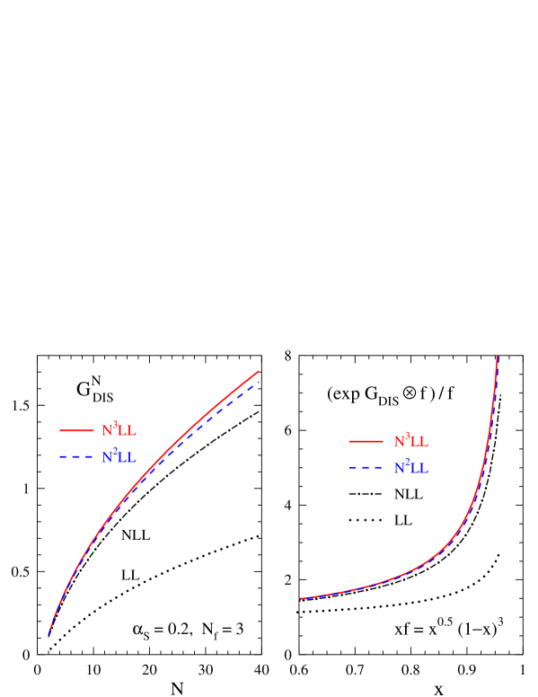
The numerical expansion of $B_{\rm q}$ in QCD is far less stable than Eq. (9),

$$B_{\rm q}(\alpha_{\rm s},{n_{\!f}}\!=\!4)\;\cong\;-0.3183\,\alpha_{\rm s}\,(1\,-\,1.227\,\alpha_{\rm s}\,-\,3.405\,\alpha_{\rm s}^{2}\,+\,\ldots)\>\>.$$ (11)

Note, however, that the large third-order contribution to $B_{\rm q}$ actually stabilizes the expansion of $G^{N}$ shown in Fig 1: for $B_{\rm q,3}=0$ and $N=40$, for example, the N³LL term would be about as large as the previous order.

Figure 1: Left: successive approximations for the resummation exponent (2) of inclusive DIS. Right: minimal-prescription [3] convolutions with a typical input shape.

The coefficients $B_{\rm g,i}$ for the gluonic jet function $J_{\,\rm g}$ are, for instance, relevant in direct-photon production which is dominated by the $\,{\rm q}\bar{{\rm q}}\rightarrow{\rm g}\gamma\,$ and $\,{\rm qg}\rightarrow{\rm q}\gamma\,$ subprocesses close to threshold, see Ref. [28]. These coefficients can be obtained in the same manner as Eqs. (3), but from DIS by exchange of a scalar $\phi$ with a pointlike coupling to gluons, like the Higgs boson in limit of a heavy top quark. We have derived the corresponding coefficient function $C_{\phi,\rm DIS}$ up to the third order in the course of calculating the lower row of the flavour-singlet splitting function matrix [25]. Comparison of these results to the expansion of Eq. (1) yields $B_{\rm g,1}$ and the previously unknown quantities $B_{\rm g,2}$ and $B_{\rm g,3}$. The analytic results can be found in Ref. [5]. Here we confine ourselves to the numerical expansion in four-flavour QCD,

$$B_{\rm g}(\alpha_{\rm s},{n_{\!f}}\!=\!4)\;\cong\;-0.6631\,\alpha_{\rm s}\,(1\,-\,0.7651\,\alpha_{\rm s}\,-\,2.696\,\alpha_{\rm s}^{2}\,+\,\ldots)\>\>,$$ (12)

which shows a third-order enhancement similar to that in Eq. (11).

Finally we address the process-dependent coefficients $D_{\>\!\rm i}$ due to the large-angle emission of soft gluons. Up to now, the two-loop coefficient functions for proton-proton processes are known only for the Drell-Yan cross section and Higgs boson production in the heavy-top approximation [29, 30, 31, 32]. The corresponding coefficients $D_{\>\!2}^{\rm\{DY,H\}}$ have been extracted from these results in Refs. [20, 21]. Even for these processes, the three-loop coefficient functions have not been calculated so far. It is possible, however, to derive their third-order coefficients $D_{3}$ from mass-factorization constraints [6], using our recent results for the pole terms of the three-loop quark and gluon form factors [7, 8] and the third-order splitting functions [24, 25]. Postponing the discussion of this derivation to section 5, the results for DY case read

$$D_{1}^{\,\rm DY} = 0\>\>,$$

$$D_{2}^{\,\rm DY} = {C_{F}}\left[{C_{\!A}}\left(-\frac{1616}{27}+\frac{176}{3}\,{\zeta_{2}}+56\,{\zeta_{3}}\right)\>+\>{n_{\!f}}\left(\frac{224}{27}-\frac{32}{3}\,{\zeta_{2}}\right)\right]\>\>,$$

$$D_{3}^{\,\rm DY} = {C_{F}}{C^{\,2}_{\!A}}\left[-{594058\over 729}+{98224\over 81}\,{\zeta_{2}}+{40144\over 27}\,{\zeta_{3}}-{2992\over 15}\,{\zeta_{2}^{\,2}}-{352\over 3}\,{\zeta_{2}}{\zeta_{3}}\right.$$ (13)

$$\mbox{}-384\,{\zeta_{5}}\biggr{]}+{C_{F}}{C_{\!A}}{n_{\!f}}\left[{125252\over 729}-{29392\over 81}\,{\zeta_{2}}-{2480\over 9}\,{\zeta_{3}}+{736\over 15}\,{\zeta_{2}^{\,2}}\right]$$

$$\mbox{}+{C^{\,2}_{F}}{n_{\!f}}\left[{3422\over 27}-32\,{\zeta_{2}}-{608\over 9}\,{\zeta_{3}}-{64\over 5}\,{\zeta_{2}^{\,2}}\right]$$

$$\mbox{}+{C_{F}}{n^{\,2}_{\!f}}\left[-{3712\over 729}+{640\over 27}\,{\zeta_{2}}+{320\over 27}\,{\zeta_{3}}\right]\>\>.$$

The corresponding coefficients for Higgs boson production via gluon-gluon fusion are found to be related to these results by a simple colour-factor substitution,

$$D_{\>\!\rm i}^{\,\rm H}\;=\;{C_{\!A}}/{C_{F}}\;D_{\>\!\rm i}^{\,\rm DY}\;,$$ (14)

which is in complete analogy to Eq. (7). It worth pointing out that both the cusp anomalous dimensions $A_{\rm p}$ and the coefficients $D^{\>\!\rm DY}$ and $D^{\>\!\rm H}$ exhibit a maximally non-abelian colour structure, as anticipated for $A_{\rm p}$ in Ref. [22].

The numerical expansion of $D^{\>\!\rm DY}$ in four-flavour QCD is given by

$$D^{\>\!\rm DY}(\alpha_{\rm s},{n_{\!f}}\!=\!4)\;\cong\;2.3211\,\alpha_{\rm s}\,(0\,+\,\alpha_{\rm s}\>+\,2.675\>\alpha_{\rm s}^{2}\,+\,\ldots)\>\>.$$ (15)

The ratio of the third- and second-order coefficients is very similar to that for the jet function in Eq. (11), underlining the numerical relevance of $D_{3}$.

4 On-shell form factors and their exponentiation

The form factors of quarks and gluons are gauge invariant (but infrared divergent) parts of the perturbative corrections to inclusive hard scattering processes. They summarize the QCD corrections to the $qqX$ and $ggX$ vertices with a colour-neutral particle $X$ of either space-like or time-like momentum $q$. These quantities are also key ingredients in the infrared factorization of general higher-order amplitudes [33, 34].

The relevant amplitude for the space-like $\gamma^{\ast}\!qq$ case is

$$\Gamma_{\mu}\>=\>{\rm i}e_{\rm q}\,\bigl{(}{\bar{u}}\,\gamma_{\mu\,}u\bigr{)}\,{\cal F}_{\rm q}(\alpha_{\rm s},Q^{2})\;,$$ (16)

where $e_{\rm q}$ represents the quark charge and $Q^{2}=-q^{2}$ the virtuality of the photon. The gauge-invariant scalar function ${\cal F}_{\rm q}$ is the space-like quark form factor which can be calculated order by order in the strong coupling in dimensional regularization with $D=4-2\epsilon$. The corresponding $H\>\!\!gg$ vertex defining ${\cal F}_{\rm g}$ is an effective interaction in the limit of a heavy top quark,

$${\cal L}_{\rm eff}\;=\;-\frac{1}{4}\,C_{H}\,H\,G^{\,a}_{\mu\nu}G^{\,a,\mu\nu}\>\>,$$ (17)

where $G^{\,a}_{\mu\nu}$ denotes the gluon field strength tensor, and the prefactor $C_{H}$ includes all QCD corrections, known to N³LO [35], to the top-quark loop.

The well-known exponentiation of the form factors ${\cal F}$ is achieved by solving the evolution equations [9, 10, 11]

$$Q^{2}{\partial\over\partial Q^{2}}\ln{\cal F}\!\left(\alpha_{\rm s},{Q^{2}\over\mu^{2}},\epsilon\right)\>=\>{1\over 2}\>K(\alpha_{\rm s},\epsilon)+{1\over 2}\>G\left({Q^{2}\over\mu^{2}},\alpha_{\rm s},\epsilon\right)$$ (18)

based on a factorization of the form factor ${\cal F}$ into two functions $K$ and $G$. The latter are subject to renormalization group equations [9] which are both governed by the same anomalous dimension $A_{\rm p}$ of Eqs. (3) and (7) because, obviously, the sum of $G$ and $K$ in Eq. (18) is a renormalization-group invariant. We follow the decomposition of Refs. [11, 36], where the function $K$ is a pure counter-term collecting the infrared $1/\epsilon$ poles, while the infrared-finite function $G$ includes all dependence on the scale $Q^{2}$.

The resummed form factor is given as a double integral with the boundary condition ${\cal F}(\alpha_{s},0,\epsilon)=1$ [11]. After both integrations are performed, $\ln{\cal F}$ exhibits double logarithms of $Q^{2}/\mu^{2}$ and double poles in $\epsilon$. The relation (18) can be then used for a finite-order expansion and matching of the predictions to the results of explicit higher-order calculations. The resulting expressions for the bare expansion coefficients ${\cal F}_{\rm i}$ in terms of the quantities $A_{\rm i}$ and the (still $\epsilon$-dependent) $\alpha_{\rm s}$-expansion coefficients $G_{\rm i}$ of $G(Q^{2}/\mu^{2}=1)$ in Eq. (18) are sketched below (see Ref. [7] for the complete formulae):

$${\cal F}_{1} \!=\! -{1\over 2\epsilon^{2}}\*A_{1}-{1\over 2\epsilon}\*G_{1}$$

$${\cal F}_{2} \!\!=\!\! {1\over 8\epsilon^{4}}\*A_{1}^{2}+{1\over 8\epsilon^{3}}\*A_{1}\*(2\*G_{1}-\beta_{0})+{1\over 8\epsilon^{2}}\*(G_{1}^{2}+\ldots-A_{2})-{1\over 4\epsilon}\*G_{2}$$

$${\cal F}_{3} \!\!=\!\! -{1\over 48\epsilon^{6}}\*A_{1}^{3}+\ldots+{1\over 72\epsilon^{2}}\*(9\*G_{1}\*G_{2}+\ldots-4\*A_{3})-{1\over 6\epsilon}\*G_{3}$$

$${\cal F}_{4} \!\!=\!\! {1\over 384\epsilon^{8}}\*A_{1}^{4}+\ldots+{1\over 96\epsilon^{2}}\*(3\*G_{2}^{2}+8\*G_{1}\*G_{3}+\ldots-3\*A_{4})-{1\over 8\epsilon}\*G_{4}\>\>.\;\;$$ (19)

We have extracted all three-loop pole terms of the quark and gluon form factors ${\cal F}_{\rm\!q}$ and ${\cal F}_{\rm\!g}$ from the calculation of the third-order coefficient functions for DIS by the exchange of a photon (coupling to quarks) and a scalar $\phi$ (coupling to gluons) [26], already mentioned above in the discussion of the jet function $J_{\rm p}$. The details will be reviewed in the next section.

Similar to the two-loop analysis of Ref. [12], we write the coefficients $G_{\rm p}$ as

$$G_{\rm p,1} = 2\left(P_{\rm p,\,1}^{\,\delta}-\>\delta_{\rm pg}\beta_{0}\right)\>\>+f_{1}^{\,\rm p}+\epsilon\widetilde{G_{\rm p,1}}\>\>,$$

$$G_{\rm p,2} = 2\left(P_{\rm p,\,2}^{\,\delta}-2\delta_{\rm pg}\beta_{1}\right)+f_{2}^{\,\rm p}+\beta_{0}\widetilde{G_{\rm p,1}}(\epsilon\!=\!0)+\epsilon\widetilde{G_{\rm p,2}}\>\>,$$

$$G_{\rm p,3} = 2\left(P_{\rm p,\,3}^{\,\delta}-3\delta_{\rm pg}\beta_{2}\right)+f_{3}^{\,\rm p}+\beta_{1}\widetilde{G_{\rm p,1}}(\epsilon\!=\!0)$$ (20)

$$\mbox{{}}+\beta_{0}\Big{[}\widetilde{G_{\rm p,2}}(\epsilon\!=\!0)-\beta_{0}\widetilde{\widetilde{G_{\rm p,1}}}(\epsilon\!=\!0)\Big{]}+\epsilon\widetilde{G_{\rm p,3}}$$

with $\widetilde{F}=\epsilon^{-1}\left[\,F-F(\epsilon\!=\!0)\,\right]$. The quantities $P_{\rm p}^{\,\delta}$ have been defined in Eq. (5) above, and the terms with $\delta_{\rm pg}$ are due to the renormalization of the operator $G_{\mu\nu}G^{\mu\nu}$ in Eq. (17). The crucial point of the decomposition (4) is that the functions $f_{i}^{\,\rm p}$ turn out to be universal and, like the $A_{\rm p}$ in Eqs. (3) and (7) maximally non-Abelian with (at least up to the third order)

$$f_{i}^{\,\rm g}\;=\;{C_{\!A}}/{C_{F}}\;f_{i}^{\,\rm q}\;.$$ (21)

The explicit results for the quark case read

$$f_{1}^{\,\rm q} = 0\>\>,\quad f_{2}^{\,\rm q}\;=\;2{C_{F}}\left\{-\beta_{0}{\zeta_{2}}-\frac{56}{27}\,{n_{\!f}}+{C_{\!A}}\left(\frac{404}{27}-14{\zeta_{3}}\right)\right\}\>\>,$$

$$f_{3}^{\,\rm q} = {C_{F}}{C^{\,2}_{\!A}}\left({136781\over 729}-{12650\over 81}\,{\zeta_{2}}-{1316\over 3}\,{\zeta_{3}}+{352\over 5}\,{\zeta_{2}^{\,2}}+{176\over 3}\,{\zeta_{2}}{\zeta_{3}}+192\,{\zeta_{5}}\!\right)$$ (22)

$$\mbox{{}}+{C_{\!A}}{C_{F}}{n_{\!f}}\left(-{11842\over 729}+{2828\over 81}\,{\zeta_{2}}+{728\over 27}\,{\zeta_{3}}-{96\over 5}\,{\zeta_{2}^{\,2}}\!\right)+{C^{\,2}_{F}}{n_{\!f}}\left(-{1711\over 27}\right.$$

$$\left.\mbox{}+4\,{\zeta_{2}}+{304\over 9}\,{\zeta_{3}}+{32\over 5}\,{\zeta_{2}^{\,2}}\!\right)+{C_{F}}{n^{\,2}_{\!f}}\left(-{2080\over 729}-{40\over 27}\,{\zeta_{2}}+{112\over 27}\,{\zeta_{3}}\!\right)\>\>.$$

Note that $f_{2}^{\,\rm q}$ has been obtained already in Ref. [12], and that the coefficients of the highest $\zeta$-function weights, ${\zeta_{2}}{\zeta_{3}}$ and ${\zeta_{5}}$ at three loops, agree with the results inferred from the recent ${\cal N}\!=\!4\,$ SYM calculation in Ref. [13].

Going back to Eq. (4), it is worth noting that the leading term of $G_{3}$ in Eq. (4), together with corresponding coefficients of $G_{1}$ and $G_{2}$ to higher powers in $\epsilon$ (see Refs. [7, 8] for the explicit results) fix the six highest poles of the form factors at four loops and, in fact, at all higher orders. Moreover, taking into account that the numerical effect of $A_{4}$ in Eq. (9) is small, our present results are sufficient for deriving the infrared finite absolute ratio $|{\cal F}_{\rm p}(q^{2})/{\cal F}_{\rm p}(-q^{2})|^{2}$ of the time-like and space-like form factors up to the fourth order in $\alpha_{\rm s}$. The corresponding numerical results for ${n_{\!f}}=4,\,5$ read

$$q\bar{q}\gamma^{\ast} \!: 1+2.094\,\alpha_{\rm s}+5.613\>\alpha_{\rm s}^{\,2}+15.70\,\alpha_{\rm s}^{\,3}+(48.63\pm 0.43)\,\alpha_{\rm s}^{\,4}\;,$$

$$ggH \!: 1+4.712\,\alpha_{\rm s}+13.69\,\alpha_{\rm s}^{\,2}+25.94\,\alpha_{\rm s}^{\,3}+(36.65\pm 0.35)\,\alpha_{\rm s}^{\,4}\;,$$ (23)

where the the uncertainty of the last terms is due that of the fourth-order cusp anomalous dimensions $A_{\rm p,4}$, as estimated below Eq. (8) in section 2.

5 Partonic cross section and their infrared pole structure

In this section, we finally discuss the extraction of the form factors from our calculation of the coefficient functions for inclusive DIS and the related derivation of all soft-enhanced third-order terms for the Drell-Yan process and Higgs production, and thus of $D_{3}$ given already in Eqs. (3) and (14), from these form-factor results and mass-factorization constraints [6].

The starting points for the first step are the explicit results for the bare (unrenormalized and unfactorized) partonic structure functions $F^{\rm b}$ for $\,\gamma^{\ast}{\rm q}\rightarrow{\rm q}X\,$ and $\,\phi^{\,\ast}{\rm g}\rightarrow{\rm g}X\,$ in the limit $x\rightarrow 1$ [26]. At each order $\alpha_{\rm s}^{\,n}$ keeping only the singular pieces proportional to $\delta(1-x)$ and the +-distributions

$${\cal D}_{\>\!l}\>=\>\left[\frac{\ln^{\,l}(1-x)}{(1-x)}\right]_{+}\>\>,\quad\quad l\>=\>1,\,\ldots\,2n-1\;,$$ (24)

these results are compared to the general structure of the $n$-th order contribution $F^{\rm b}_{n}$ in terms of the $l$-loop form factors ${\cal F}_{l}$ and the corresponding real-emission parts ${\cal S}_{l\,}$,

$$F^{\rm b}_{0} \,=\, \delta(1-x)$$

$$F^{\rm b}_{1} \,=\, 2{\cal F}_{1}\,\delta(1-x)+{\cal S}_{1}$$

$$F^{\rm b}_{2} \,=\, \left(2{\cal F}_{2}+{\cal F}_{1}^{\,2}\right)\delta(1-x)+2{\cal F}_{1}{\cal S}_{1}+{\cal S}_{2}$$

$$F^{\rm b}_{3} \,=\, \left(2{\cal F}_{3}+2{\cal F}_{1}{\cal F}_{2}\right)\delta(1-x)+\left(2{\cal F}_{2}+{\cal F}_{1}^{\,2}\right){\cal S}_{1}+2{\cal F}_{1}{\cal S}_{2}+{\cal S}_{3}\;.\quad$$ (25)

In DIS the $x$-dependence of the real emission factors ${\cal S}_{k}$ is of the form ${\cal S}_{k}(f_{k,\epsilon})$, with the $D$-dimensional +-distributions $f_{k,\epsilon}$ defined by

$$f_{k,\epsilon}(x)\;=\;\epsilon[\,(1-x)^{-1-k\epsilon}\,]_{+}\;=\;-{1\over k}\,\delta(1-x)+\sum_{i=0}\,{(-k\epsilon)^{i}\over i\,!}\,\epsilon\,{\cal D}_{\>\!i}\;.$$ (26)

The dimensionally regularized (with $D=4-2\epsilon$) bare structure functions $F^{\rm b}_{n}$ in Eq. (25) exhibit poles in $\epsilon$ up to $\epsilon^{-2n}$, with a structure completely determined by mass factorization. On the other hand, the individual real and virtual contributions ${\cal F}_{k}$ and ${\cal S}_{k}$ in Eq. (25) contain poles up to order $\epsilon^{-2k}$, which cancel due to the Kinoshita–Lee-Nauenberg theorem [37, 38].

The determination of the form factor now proceeds as follows. Once the combinations of lower-order quantities in Eq. (25) have been subtracted from $F^{\rm b}_{n}$, the $n$-loop form factor ${\cal F}_{n}$ can simply be extracted by the substitution

$${\cal D}_{\>\!0}\>\to\>{1\over n\epsilon}\,\delta(1-x)-\sum_{i=1}\,{(-n\epsilon)^{i}\over i\,!}\,{\cal D}_{\>\!i}\;,$$ (27)

which exploits the particular analytical dependence of ${\cal S}_{k}$ on $x$, i.e., Eq. (26). As $\delta(1-x)$ enters with a factor $1/\epsilon$, this extraction loses one power in $\epsilon$. Hence from the third-order calculation to order $\epsilon^{0}$, as performed for the coefficient function, we can only extract all pole terms of ${\cal F}_{3}$ in this manner.

The second step, the determination of the +-distribution contributions to coefficient functions for lepton-pair and and Higgs boson production, proceeds along similar lines, see Ref. [39] for an early two-loop application to the Drell-Yan process. In analogy to Eq. (25), the soft limit of the bare partonic cross sections $W^{\rm b}$ for $\,{\rm q}\bar{{\rm q}}\,\rightarrow\,\gamma^{\ast}\,\rightarrow\,l^{+}l^{-}\,$ and $\,{\rm gg}\,\rightarrow\,H\,$ reads

$$W^{\rm b}_{0} \,=\, \delta(1-x)$$

$$W^{\rm b}_{1} \,=\, 2\,\mbox{Re}\,{\cal F}_{1}\,\delta(1-x)+{\cal S}_{1}$$

$$W^{\rm b}_{2} \,=\, (2\,\mbox{Re}\,{\cal F}_{2}+\left|{\cal F}_{1}\right|^{2})\,\delta(1-x)+2\,\mbox{Re}\,{\cal F}_{1}{\cal S}_{1}+{\cal S}_{2}$$

$$W^{\rm b}_{3} \,=\, (2\,\mbox{Re}\,{\cal F}_{3}+2\left|{\cal F}_{1}{\cal F}_{2}\right|)\,\delta(1-x)+(2\,\mbox{Re}\,{\cal F}_{2}+\left|{\cal F}_{1}\right|^{2}){\cal S}_{1}$$ (28)

$$\mbox{}+2\,\mbox{Re}\,{\cal F}_{1}{\cal S}_{2}+{\cal S}_{3}\;,$$

where, of course, ${\cal F}$ now denotes the time-like quark or gluon form factor, known by analytic continuation from $q^{2}=-Q^{2}<0\,$ to $q^{2}>0$. The real-emission contributions ${\cal S}_{k}$ depend on the scaling variable $x=M_{\gamma^{\,\ast}\!,\,H}^{\,2}/s$. In this case, the dependence of ${\cal S}_{k}$ on $x$ is of the form ${\cal S}_{k}(f_{2k,\epsilon})$, i.e.,

$${\cal S}_{k}\;=\;f_{2k,\epsilon}\,\sum_{l=-2k}^{\infty}2k\,s_{k,l}\>\epsilon^{\,l}\;.$$ (29)

With the known time-like form factors, the expansion coefficients $s_{k,l}$ of the soft function ${\cal S}_{k}$ can be derived recursively as far as they are subject to the KLN cancellations and the mass-factorization structure relating the remaining poles to the splitting functions (5). Employing the results of Refs. [7, 8] and [24, 25], the third-order terms $s_{3,-6}\,\ldots\,s_{3,-1}$ can be obtained. Due to Eq. (26) this is sufficient to derive all +-distribution contributions to the third-order coefficient functions, in particular also the coefficient of ${\cal D}_{0}$ from which $D_{3}^{\{\rm DY,\rm H\}}$ in Eqs. (3) and (14), can be determined by matching. 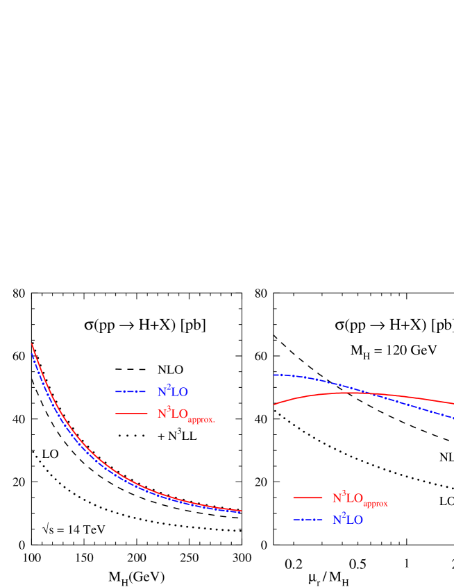An important application on these new results is presented in Fig. 2.

The connection between mass-factorization and resummation leads to a simple relation between the coefficients $D_{\rm n}$ and $f_{\rm n}^{\>\!\rm p}$ in Eqs. (21) and (4),

$$D_{2}^{\,\{\rm DY,\,\rm H\}} = -2f_{2}+2\beta_{0}s_{1,0}$$

$$D_{3}^{\,\{\rm DY,\,\rm H\}} = -2f_{3}+2\beta_{1}s_{1,0}-4\beta_{0}^{2}s_{1,1}+4\beta_{0}\!\left[s_{2,0}-{36\over 5}\,{\zeta_{2}^{\,2}}\,C_{\{F,A\}}^{\,2}\right]\;,\>\>$$ (30)

which has also been derived by extending the threshold resummation to the $N$-independent contributions [40, 41], see also Ref. [42]. In our approach, the $s_{n,l}$ terms can be traced back to the $\alpha_{\rm s}$-renormalization of Eqs. (5).

Figure 2: The perturbative expansion of the total cross section for Higgs production at the LHC. Left: dependence on the Higgs mass $M_{\rm H}$. Right: renormalization-scale (in-) stability for $M_{\rm H}=120\mbox{ GeV}$. See Ref. [6] for a detailed discussion.

6 Summary

Building on our third-order computation of the splitting functions [24, 25] and the coefficient functions for inclusive DIS [26], we have derived new three-loop and all-order results for the threshold resummation [5, 6], the on-shell quark and gluon form factors [7, 8], and the coefficient functions for lepton-pair and Higgs boson production at proton colliders [6]. These results have important implications within and beyond perturbative QCD.