Scalar mesons on the Lattice

Sasa Prelovsek

Department of Physics, University of Ljubljana, Jadranska 19, 1000 Ljubljana, Slovenia

and

Institute Jozef Stefan, Jamova 39, 1000 Ljubljana, Slovenia

Abstract

The simulations of the light scalar mesons on the lattice are presented at the introductory level. The methods for determining the scalar meson masses are described. The problems related to some of these methods are presented and their solutions discussed.

1 Introduction

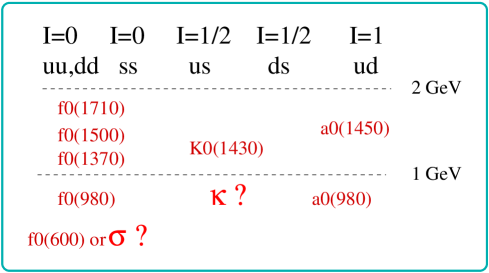
The observed spectrum of the light scalar resonances below $2$ GeV is shown in Fig. 1. The existence of flavor singlet $\sigma$ and strange iso-doublet $\kappa$ are still very controversial [1]. Irrespective of their existence, it is difficult to describe all the observed resonances by one or two $SU(3)$ flavor nontes of $\bar{q}q$ states:

• If $\sigma$ and $\kappa$ do not exist, than $K_{0}(1430)$ has to be strange partner of $a_{0}(980)$, but the mass difference appears to big. Also there are to many states to be described by one nonet.

• If $\sigma$ and $\kappa$ exist, then all these states could represent two $\bar{q}q$ nonets and one glueball, where the largest glueball component is commonly attributed to $f_{0}(1500)$. However, most of the models and lattice simulations have difficulties in relating the observed properties of states below $1$ GeV to the $\bar{q}q$ states.

This situation is in contrast to the spectrum of light pseudoscalar, vector and axial-vector resonances, where $\bar{q}q$ assignment works well. It raises a question whether the scalar resonances below $1$ GeV are conventional $\bar{q}q$ states or perhaps exotic states such as tetraquarks [2].

This issues could be settled if the mass of the lightest $\bar{q}q$ states could be reliably determined on the lattice and identified with the observed resonances. In lattice QCD, the hadron masses are conventionally extracted from the correlation functions that are computed on the discretized space-time.

Figure 1: The spectrum of observed light scalar resonances below $2$ GeV [1]. The existence of $\sigma$ and $\kappa$ are still very controversial experimentally.

In the next section we present how the scalar correlator is calculated on the lattice. The relation between the scalar correlator and the scalar meson mass is derived in Section 3. A result for the mass of $I=1$ scalar meson is presented in Section 4. In Section 5 we point out the problems which arise due to the unphysical approximations that are often used in the lattice simulations and we discuss the proposed solutions. We close with Conclusions.

This article follows the introductory spirit of the talk given at the Workshop Exciting hadrons¹ and many technical details are omitted.

2 Calculation of the scalar correlator

Let us consider the correlation function for a flavor non-singlet scalar meson $\bar{q}_{1}q_{2}$ first. In a lattice simulation it is calculated using the Feynman functional integral on a discretized space-time of finite volume and finite lattice spacing. The correlation function represents a creation of a pair $\bar{q}_{1}q_{2}$ with $J^{P}=0^{+}$ at time zero and annihilation of the same pair at some later Euclidean time $t$

$$C(t)=\sum_{\vec{x}}\langle 0|\bar{q}_{1}(\vec{x},t)q_{2}(\vec{x},t)~{}\bar{q}_{2}(\vec{0},0)q_{1}(\vec{0},0)|0\rangle~{},$$ (1)

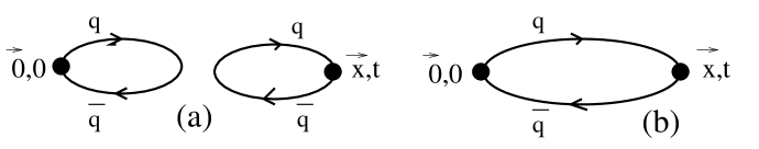
where both quarks are created (annihilated) at the same spatial point for definiteness here. Wick contraction relates this to the product of two quark propagators shown by the connected diagram in Fig. 2b

$$C(t) =\bigl{\langle}C_{G}(t)\bigr{\rangle}_{G}$$ (2)

$$C_{G}(t) =\sum_{\vec{x}}{\rm Tr}_{s,c}\bigl{[}{\rm Prop}^{2}_{\vec{0},0\to\vec{x},t}~{}{\rm Prop}^{1}_{\vec{x},t\to\vec{0},0}\bigr{]}\!=\sum_{\vec{x}}{\rm Tr}_{s,c}\bigl{[}{\rm Prop}^{2}_{\vec{0},0\to\vec{x},t}\gamma_{5}{\rm Prop}^{1~{}\dagger}_{\vec{0},0\to\vec{x},t}\gamma_{5}\bigr{]}~{}.$$

The quark propagator in the gluon field $G$ and Euclidean space-time [3]

$${\rm Prop^{i}}_{\vec{x},x_{0}\to\vec{y},y_{0}}=\biggl{(}\frac{1}{{\not{\!\!D_{E}}}+m_{i}}\biggr{)}_{\vec{x},x_{0}\to\vec{y},y_{0}}$$ (3)

is the inverse of the discretized Dirac operator ${\not{\!\!D_{E}}}+m_{i}~{}$, which is a matrix in coordinate space and depends on the gluon field $G$ . The inversion of a large Dirac matrix is numerically costly, but the calculation of correlator (2) is feasible since it depends only on two propagators from a certain point $(\vec{0},0)$ to all points $(\vec{x},t)$. Both of these are obtained by solving the equation $({\not{\!\!D_{E}}}+m_{i})V^{\prime}=V$ for a single source vector $V$ which is non-zero only at $(\vec{0},0)$. The expectation value over the gluon fields in (2) is computed based on the Feynman functional integral

$$C(t)=\frac{\int{\cal D}G~{}C_{G}(t)~{}\int{\cal D}q\int{\cal D}\bar{q}~{}e^{-S_{QCD}}}{\int{\cal D}G\int{\cal D}q\int{\cal D}\bar{q}~{}e^{-S_{QCD}}}=\frac{\int{\cal D}G~{}C_{G}(t)~{}\Pi_{i}{\rm det}[{\not{\!\!D_{E}}}+m_{i}]~{}e^{-S_{G}}}{\int{\cal D}G~{}\Pi_{i}{\rm det}[{\not{\!\!D_{E}}}+m_{i}]~{}e^{-S_{G}}}~{}.$$ (4)

A finite ensemble of $N$ gluon field configurations is generated in the lattice simulations. Each configuration is generated with a probability $\Pi_{i}{\rm det}[{\not{\!\!D_{E}}}+m_{i}]~{}e^{-S_{G}}$ for a given discretized gauge action $S_{G}$ and Dirac operator ${\not{\!\!D_{E}}}$. The functional integral (4) is calculated as a sum over the ensemble

$$C(t)=\frac{1}{N}\sum_{j=1}^{N}C_{G_{j}}(t)~{}.$$ (5)

Figure 2: The disconnected (a) and the connected (b) Feynman diagrams that need to be evaluated to compute the correlator. The disconnected diagram is present only for the flavor singlet meson.

The correlator for the flavor singlet scalar meson $\bar{q}q$

$$C(t)=\sum_{\vec{x}}\langle 0|\bar{q}(\vec{x},t)q(\vec{x},t)~{}\bar{q}(\vec{0},0)q(\vec{0},0)|0\rangle~{}$$ (6)

requires also the calculation of the disconnected diagram in Fig. 2a

$$\biggl{\langle}{\rm Tr}_{s,c}{\rm Prop}_{\vec{0},0\to\vec{0},0}~{}\sum_{\vec{x}}{\rm Tr}_{s,c}{\rm Prop}_{\vec{x},t\to\vec{x},t}\biggr{\rangle}_{G}$$ (7)

in addition to connected one. The propagator ${\rm Prop}_{\vec{x},t\to\vec{x},t}$ in principle requires the solution of $({\not{\!\!D_{E}}}+m_{i})V^{\prime}=V$ for source vector $V$ at any point. Such a number of inversions is normally prohibitively large and one is forced to use approximate methods for evaluating the disconnected part (7) of the singlet correlator. A calculation of the correlator for singlet meson in therefore much more demanding than for non-singlet meson.

3 Relation between correlator and meson mass

In this Section we derive the relation between the scalar correlator and the scalar meson mass. The state $\bar{q}(\vec{0})q(\vec{0})|0\rangle$ that is created at time zero is not a scalar meson $|S\rangle$, but it is a superposition of the scalar meson and all the other eigenstates of Hamiltonian $|n\rangle$ with the same quantum numbers $J^{P}=0^{+}$ and $I^{G}$ as $|\bar{q}q\rangle$

$$|\bar{q}q\rangle=\sum_{n}c_{n}|n\rangle=c_{1}|S\rangle+c_{2}|S^{*}\rangle+\sum c_{i}\biggl{|}{\rm\small{multi\atop hadron\ st.}}\biggr{\rangle}_{i}+...\biggl{(}+c_{0}|0\rangle\ {\rm\small{only\ for\atop singlet}}\biggr{)}~{}.$$ (8)

Here $|S\rangle$ and $|S^{*}\rangle$ are ground and excited scalar mesons, while the third term represents the sum over multi-hadron states. The eigenstate $|n\rangle$ evolves as $e^{i\vec{p}_{n}\vec{x}-E_{n}t}$ in Euclidean space-time, so the scalar correlators (1) and (6) evolve as

$$C(t) =\!\!\sum_{\vec{x}}\langle\bar{q}(\vec{x},t)q(\vec{x},t)~{}\bar{q}(\vec{0},0)q(\vec{0},0)\rangle=\!\!\sum_{n}\sum_{\vec{x}}\langle\bar{q}q|n\rangle e^{i\vec{p}_{n}\vec{x}-E_{n}t}\langle n|\bar{q}q\rangle=\!\!\sum_{n}|\langle\bar{q}q|n\rangle|^{2}~{}e^{-E_{n}t}\bigl{|}_{\vec{p}=0}$$

$$=|c_{1}|^{2}e^{-m_{S}t}+|c_{2}|^{2}e^{-m_{S^{*}}t}+\sum|c_{i}|^{2}e^{-E^{\rm{multi\atop had.}}_{i}t}+...\biggl{(}+|c_{0}|^{2}\ {\rm\small{only\ for\atop singlet}}\biggr{)}~{}.$$ (9)

If $|S\rangle$ is the lightest state among $|n\rangle$, than $C(t)\propto e^{-m_{S}t}$ at large $t$ and $m_{S}$ and can be extracted simply by fitting the lattice correlator to the exponential time dependence.

In the case of the flavor singlet correlator, the lightest state in the sum (8) is the vacuum state. Its corresponding coefficient $c_{0}$ (8) is the scalar condensate $\langle\bar{q}q\rangle$. Another important light state that contributes at large $t$ is $\pi\pi$, so extraction of $m_{\sigma}$ requires the fit to

$$C(t)\stackrel{{\scriptstyle t\to\infty}}{{=}}|c_{\sigma}|^{2}e^{-m_{\sigma}t}+\sum_{\vec{p}_{\pi}}\bigl{|}c_{\vec{p}_{\pi}}\bigr{|}^{2}e^{-E^{\pi\pi}_{\vec{p}_{\pi}}t}+\langle\bar{q}q\rangle^{2}~{}.$$ (10)

The extraction of $m_{\sigma}$ is very challenging since $C(t)$ requires the calculation of the disconnected diagram (see previous Section) and since RHS in (10) is largely dominated by $\langle\bar{q}q\rangle^{2}$.

These two problems do not affect the study of the flavor non-singlet meson. However, even in this case there are several multi-hadron states which are light and need to be taken into account in the fit of the correlator (3) at large $t$ in order to extract $m_{S}$. The lightest multi-hadrons states with $J^{P}=0^{+}$ are two-pseudoscalar states in $S$-wave. In case of $I=1$ correlator, the contribution of scalar meson $a_{0}$ is accompanied by contributions of $\pi\eta$, $\bar{K}K$ and $\pi\eta^{\prime}$ in three-flavor QCD. Let us note that in nature these three states are lighter than observed resonance $a_{0}(1450)$; the state $\pi\eta$ is also lighter than observed resonance $a_{0}(980)$. In two-flavor QCD, the only two-pseudoscalar state $\pi\eta^{\prime}$ is relatively heavy and not so disturbing for the extraction of $m_{a0}$ from (3).

The above derivation of time-dependence for a correlator was based on QCD, which is a proper unitary field theory. The resulting correlator (3) is positive definite. Let us point out that certain approximations used in lattice simulations (quenching, partial quenching, staggered fermions, mixed-quark actions) break unitarity and may render negative correlation function. These approximations will be discussed in Section 5 together with the necessary modifications of the fitting formula (3).

4 Mass of scalar meson with I=1

A lattice simulation of the scalar meson $a_{0}$ with $I=1$ [4] is presented in this section, as an example. It employs two dynamical quarks, lattice spacing $0.12$ fm, lattice volume $16^{3}\times 32$ and ensemble of about $100$ gauge configurations [4, 5]. The advantage of simulation [4] is that its discretized (Domain-Wall) fermion action has good chiral properties: it is invariant under the chiral transformation for $m_{q}=0$ even at finite lattice spacing, which is not the case for some of the commonly used discretized fermion actions. Another advantage of the simulation with two dynamical quarks [4] is that the exponential fit of the correlator at large $t$ renders $m_{a0}$. The conventional exponential fit is justified in this case since the only two-pseudoscalar intermediate state in two-flavor QCD is $\pi\eta^{\prime}$, which is relatively heavy and does not affect the extraction of $m_{a0}$ (see previous Section).

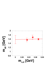
The resulting mass is presented in Fig. 3 for different input masses $m_{u,d}$, where isospin limit $m_{u}=m_{d}$ is employed. There are no simulations at physical masses $m_{u,d}$ since the pion cloud around the scalar meson with $\lambda_{\pi}=hc/140~{}$MeV$\simeq 9$ fm would be to squeezed on the lattice with extent $16\times 0.12~{}$fm$\simeq 2~{}$fm. The $u/d$ quarks and pions are heavier in simulation than in the nature in order to avoid large finite volume effects. The linear extrapolation of $m_{a0}$ to the physical quark mass $m_{u,d}\simeq 4~{}{\rm MeV}$ in Fig. 3 gives

$$m_{a0}=1.58\pm 0.34~{}{\rm GeV}~{}.$$ (11)

Although our result for the mass of the lightest $\bar{q}q$ state with $I=1$ has sizable error-bar, it appears to be closer to the observed resonance $a_{0}(1450)$ than to $a_{0}(980)$. It gives preference to the interpretation that $a_{0}(980)$ is not conventional $\bar{q}q$ state.

Results from other lattice simulations of the light scalar mesons can be found in [6]-[11].

Figure 3: The triangles present resulting $m_{a0}$ for three values of bare quark masses $m_{u,d}$ [4]. The dashed line is the linear extrapolation of $m_{a0}$ to the value of $m_{u,d}$ in nature.

5 Problems due to unphysical approximations

The simulation presented in the previous section is a discretized version of two-flavor QCD and does not employ any unphysical approximations except for the discretization of space-time. It renders positive definite correlation function, as expected in proper Quantum Field Theory (3).

However, lattice simulations often employ unphysical approximations which facilitate numerical evaluation. One of the indications that the simulation does not correspond to a proper QCD is the negative scalar correlator. Another sign of unphysical simulation is when $I=1$ correlator drops as $e^{-2M_{\pi}t}$ at large $t$ although the lightest two-pseudoscalar state with $I=1$ is $\pi\eta$. Both of these unphysical lattice results can occur if the theory that is being simulated is not unitary, which is the case for all the commonly used approximations listed below:

• In quenched simulation the fermion determinant in (4) is replaced by a constant. This corresponds to neglecting all the closed sea-quark loops. The $I=1$ scalar correlator is negative in this case and its negativity was attributed to the intermediate state $\pi\eta^{\prime}$ in Ref. [6]. The prediction for $\pi\eta^{\prime}$ intermediate state in quenched version of Chiral Perturbation Theory (ChPT) describes the sign and the magnitude of the lattice correlator at large $t$ well [6, 7]. The mass $m_{a0}$ was extracted [6, 7] by fitting the quenched $I=1$ correlator to the sum of $e^{-m_{a0}t}$ term and the contribution of $\pi\eta^{\prime}$ as predicted by Quenched ChPT.

• In partially quenched simulation the mass of the sea quark is different from the mass of the valence quark, although they are the same in nature. The mass of the valence quark is the mass that appears in the propagator of the correlator $C_{G}$ (2), while the mass of the sea quark is the mass that appears in the fermion determinant (4). The partially quenched scalar correlator with $I=1$ was found to be negative if $m_{val}<m_{sea}$ [4]. This was attributed to intermediate states with two pseudoscalar mesons and was described well using partially quenched version of ChPT [4]. The mass $m_{a0}$ was extracted by fitting the partially quenched correlator to the sum of $e^{-m_{a0}t}$ term and the contribution of two-pseudoscalar states as predicted by Partially Quenched ChPT [4]. The resulting mass agrees with the mass (11).

• The simulations with mixed quark actions employ different discretizations of the Dirac operator for valence and sea quarks. The method of extracting scalar meson mass from a such simulations was proposed in [12, 13].

• The simulations with staggered quarks use an artificial taste degree of freedom for quarks in order to solve fermion doubling problem [3]. The method of extracting scalar meson mass from simulations with staggered quarks [11] was proposed in [12].

All these approximations modify the contribution of two-pseudoscalar intermediate states with respect to QCD. The effects of these approximations can be therefore determined by predicting the two-pseudoscalar contributions using appropriate versions of ChPT. These analytic predictions [6, 4, 12, 13] allow the extraction of the scalar meson mass from the correlator as long as the contribution of two-pseudoscalar intermediate states does not completely dominate over the $e^{-m_{S}t}$ term.

6 Conclusions

The nature of scalar resonances below $1$ GeV is not established yet. A lattice determination of the masses for ground $\bar{q}q$ scalar states would help to resolve the problem.

In principle, the scalar mass can be extracted from the scalar correlator that is computed on the lattice. However, the interesting term $e^{-m_{S}t}$ in the correlator is accompanied by the contribution of two-pseudoscalar states $e^{-E_{PP}t}$. The problem is that the energy of two-pseudoscalar states is small, so they may dominate the correlator and complicate the extraction of scalar meson mass. On top of that, the contribution of two-pseudoscalar states is significantly affected by the unphysical approximations that are often used in lattice simulations. Luckily, these effects can be predicted using appropriate versions of Chiral Perturbation Theory and they agree with the observed effects on the lattice correlators. We give the list of references, which provide the expressions for extracting $m_{S}$ from the correlators for various types of simulations.

A simulation, which does not suffer from the problems listed above, gives $1.58\pm 0.34~{}$GeV for the mass of the lightest $\bar{q}q$ state with $I=1$. This supports the interpretation that observed $a0(1450)$ is the lightest $(\bar{q}q)_{I=1}$ state, while $a0(980)$ might be something more exotic.

References

- [1] Particle Data Group, Review of Particle Physics, Phys. Lett. B592 (2004) 1.
- [2] M.G. Alford and R.L. Jaffe, Nucl. Phys. B578 (2000) 367; L. Maiani et al., Phys. Rev. Lett. 93 (2004) 212002.
- [3] H.J. Rothe, Lattice Gauge Theories, An Introduction, World Scientific.
- [4] S. Prelovsek et al., RBC Coll., Phys. Rev. D70 (2004) 094503.
- [5] Y. Aoki et al., RBC Coll., hep-lat/0411006.
- [6] W. Bardeen et. al, Phys. Rev. D65 (2002) 014509; W. Bardeen et. al, Phys. Rev. D69 (2004) 054502.
- [7] S. Prelovsek and K. Orginos, RBC Coll., Nucl. Phys. B (Proc. Suppl.) 119 (2003) 822 [hep-lat/0209132].
- [8] W. Lee and D. Weingarten, Phys. Rev. D61 (2000) 014015.
- [9] T. Kunihiro et al., SCALAR Coll., Phys. Rev. D70 (2004) 034504.
- [10] C. McNeile and C. Michael, Phys. Rev. D63 (2001) 114503; A. Hart, C. McNeile and C. Michael, Nucl. Phys. B (Proc. Suppl.) 119 (2003) 266.
- [11] C. Bernard et al., MILC Coll., Phys. Rev. D64 (2001) 054506; C. Aubin et al., MILC Coll., Phys. Rev. D70 (2004) 094505; A. Irving et al., POS(LAT2005)027 [hep-lat/0510066].
- [12] S. Prelovsek, hep-lat/0510080.
- [13] M. Golterman and T. Izubuchi, Phys. Rev. D71 (2005) 114508.