x Renormalization Group Analysis in NRQCD for Colored Scalars

Abstract

The vNRQCD Lagrangian for colored heavy scalar fields in the fundamental representation of QCD and the renormalization group analysis of the corresponding operators are presented. The results are an important ingredient for renormalization group improved computations of scalar-antiscalar bound state energies and production rates at next-to-next-to-leading-logarithmic (NNLL) order.

I Introduction

Many models of supersymmetry (SUSY) breaking predict that at least one of the SUSY partners of the top quark is sufficiently light such that pair production is possible at a future Linear Collider with c.m. energies below 1 TeV. In such a scenario threshold studies are feasible, where squark pairs are produced with small relative velocities, and which allow for precise measurements of squark masses, lifetimes or couplings in close analogy to threshold measurements at the top-antitop pair threshold TTbarsim ; synopsis ; Habilitation . If the SUSY partner of the gluon is (as is general expected) not much lighter than the electroweak scale, then the low-energy QCD dynamics of squarks is, up to the fact that we are dealing with a colored spinless state, based on standard QCD with interactions carried by spin-1 gluons in the adjoint representation.

It is a special feature of pair production of heavy colored particles close to the two-particle threshold that multi-gluon exchange leads to singular terms $\propto(\alpha_{s}/v)^{n}$ and $\propto(\alpha_{s}\ln v)^{n}$ in the amplitude at $n$-loop perturbation theory, where $v$ is the relative particle velocity. Thus for $v\sim\alpha_{s}$, which corresponds to a region in c.m. energy of roughly $|\sqrt{s}-2m|\mathrel{\raise 1.29167pt\hbox{$<$\kern-7.5pt\lower 4.30554pt\hbox{$\sim$}}}0.1m$, $m$ being the heavy particle mass, the singular terms have to be summed to all orders in $\alpha_{s}$. This is achieved most efficiently within an effective field theory. For top pair threshold production the effective theory vNRQCD (“velocity non-relativistic QCD”) LMR ; amis2 ; HoangStewartultra was developed to carry out this summation program aiming for NNLL order precision, i.e. accounting for ${\cal O}(\alpha_{s}^{2},\alpha_{s}v,v^{2})$ QCD hmst ; hmst1 ; Hoang3loop as well as ${\cal O}(\alpha_{\rm em})$ electroweak corrections HoangReisser . For squark-antisquark pair threshold production previous studies involved leading-logarithmic (LL) precision Bigi ; Fabiano . Higher order QCD or electroweak effects were not taken into account in a systematic manner, although it is known from the top threshold that corrections to the LL approximation can be substantial.

In this work we present the vNRQCD Lagrangian for a particle-antiparticle pair of heavy non-relativistic colored scalars in the fundamental representation of QCD. We provide matching conditions and anomalous dimensions required for renormalization group improved computations of threshold pair production at next-to-leading logarithmic (NLL) order and scalar-antiscalar bound state energies at NNLL order in the non-relativistic expansion. For our presentation we follow closely the conventions and notations of Refs. LMR ; HoangStewartultra . Among the crucial elements of the construction are that vNRQCD is obtained by a single matching procedure at the hard scale $m$ and that the soft and the ultrasoft renormalization scales, $\mu_{S}$ and $\mu_{U}$, are correlated according to the non-relativistic energy-momentum relation of a heavy particle at all times. Thus we have $\mu_{U}=\mu_{S}^{2}/m=m\nu^{2}$, where $\nu$ is the dimensionless renormalization group scaling parameter of vNRQCD. (For corresponding computations in the pNRQCD approach pNRQCD2 see Ref. Pineda1 .) For convenience, for the most part of the paper, we call the scalars in the fundamental representation of QCD simply “squarks” and the scalar versions of vNRQCD and QCD frequently just vNRQCD and QCD, respectively.

The outline of the paper is as follows: In Sec. II we present the terms of the scalar vNRQCD Lagrangian relevant for this work together with their matching conditions. A special set of operators generated by ultrasoft renormalization is discussed in Sec. IIB. The running of all relevant potentials is discussed in Sec. III. Finally, Sec. IV is devoted to the anomalous dimensions of the S- and P-wave squark-antisquark production currents. Conclusions are given in Sec. V.

II Effective Theory Lagrangian

The scalar vNRQCD effective Lagrangian is written in terms of the fields $\psi_{\mathbf{p}}$ for the squark, $\chi_{\mathbf{p}}$ for the antisquark, ($A_{q}^{\mu}$, $c_{q}$, $\varphi_{q}$, $\phi_{q}$) for soft (massless) gluons, ghosts, quarks and squarks and ($A^{\mu}$, $c$, $\varphi$, $\phi$) for ultrasoft (massless) gluons, ghosts, quarks and squarks. For the light quarks and squarks we assume $n_{f}$ and $n_{s}$ light flavor components, respectively. The covariant derivative is $D^{\mu}=\partial^{\mu}+ig_{u}A^{\mu}=(D^{0},-\mathbf{D})$, with $D^{0}=\partial^{0}+ig_{u}A^{0}$, $\mathbf{D}=\nabla-ig_{u}\mathbf{A}$ and only involves the ultrasoft gluon field and the ultrasoft gauge coupling. For the representation of the (anti)squark fields and the soft fields the vNRQCD label formalism is used to separate the fluctuations at the scales $mv$ (soft) and $mv^{2}$ (ultrasoft) LMR . Thus the spatial dependence of fields refers only to ultrasoft fluctuations and, for example, for the heavy squark field we have $\partial^{\mu}\psi_{\mathbf{p}}(x)\sim mv^{2}\psi_{\mathbf{p}}(x)$, while the label $\mathbf{p}$ refers to the soft three-momentum component of the squark field.

II.1 Basic Lagrangian

The basic vNRQCD Lagrangian can be obtained by tree level matching to full QCD and can be separated into ultrasoft, soft and potential components, ${\cal L}={\cal L}_{u}+{\cal L}_{s}+{\cal L}_{p}$.

Figure 1: Effective theory diagrams for the interaction of a heavy squark with an ultrasoft gluon.

The ultrasoft piece of the effective Lagrangian describes the interactions of ultrasoft gluons with squarks (Fig. 1) and also contains the kinetic energy contributions for the squarks and the ultrasoft fields. It has the form

$${\cal L}_{u} = \sum_{\mathbf{p}}\,\bigg{\{}\psi_{\mathbf{p}}^{*}\bigg{[}iD^{0}-\frac{\left({\bf p}-i{\bf D}\right)^{2}}{2m}+\frac{{\mathbf{p}}^{4}}{8m^{3}}+\ldots\bigg{]}\psi_{\mathbf{p}}+(\psi\to\chi,T\to\bar{T})\,\bigg{\}}$$ (1)

$$-\,\frac{1}{4}G_{u}^{\mu\nu}G^{u}_{\mu\nu}+\sum_{i=1}^{n_{f}}\bar{\varphi}_{i}i\mathchoice{\hbox to0.0pt{\hss$\displaystyle/$\hss\kern-8.55695pt}\hbox{$\displaystyle D$}}{\hbox to0.0pt{\hss$\textstyle/$\hss\kern-8.55695pt}\hbox{$\textstyle D$}}{\hbox to0.0pt{\hss$\scriptstyle/$\hss\kern-5.98985pt}\hbox{$\scriptstyle D$}}{\hbox to0.0pt{\hss$\scriptscriptstyle/$\hss\kern-4.27846pt}\hbox{$\scriptscriptstyle D$}}\varphi_{i}+\sum_{i=1}^{n_{s}}(D^{\mu}\phi_{i})^{*}(D_{\mu}\phi_{i})+\ldots\,,$$

where $G_{u}^{\mu\nu}$ is the ultrasoft field strength tensor and $m$ is the heavy squark pole mass. The spatial dependence and the summation over the color indices of the fields are understood here and for the rest of this paper. To avoid double counting the interactions have to be multipole-expanded with the scaling $\mathbf{p}\sim mv$ and $\mathbf{D}\sim mv^{2}$. The form of the first term of Eq. (1) is determined by reparametrization invariance manohar ; Manoharm3 and does not receive any non-trivial renormalization factors. For the squark fields we use the non-relativistic normalization with $\psi_{\mathbf{p}}\sim\chi_{\mathbf{p}}\sim m^{3/2}$, such that the squark kinetic energy has the usual form known from NRQCD for heavy quarks and non-relativistic quantum mechanics. To the order we are working ${\cal L}_{u}$ agrees with the ultrasoft Lagrangian for the quark case. Likewise, the momentum and $v$ scaling of the effective theory squark fields and effective theory Feynman diagrams is equivalent for the heavy quark case discussed in detail in Refs. LMR ; HoangStewartultra . Here we employ the same power counting formalism. The factors of $\mu_{U}^{\epsilon}$ and $\mu_{S}^{\epsilon}$ that appear in the effective Lagrangian in $d=4-2\epsilon$ dimensions are uniquely determined by the requirement that the kinetic terms in the vNRQCD action are of order $v^{0}$ LMR ; amis2 ; HoangStewartultra . To be specific, for the squark and gluons fields this gives the scaling $\psi_{\bf p}\sim(mv)^{3/2-\epsilon}$, $A^{\mu}\sim(mv^{2})^{1-\epsilon}$, and $A_{q}^{\mu}\sim(mv)^{1-\epsilon}$. For the covariant derivative this leads to the form $D^{\mu}=\partial^{\mu}+i\mu_{U}^{\epsilon}g_{u}A^{\mu}$ in dimensional regularization.

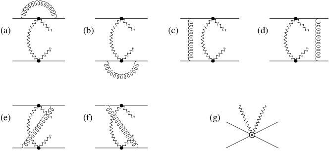
The soft Lagrangian describes interactions of soft (massless) gluons, ghosts, quarks or squarks with the heavy squarks and has terms

$${\cal L}_{s} = \sum_{q}\Big{\{}-\frac{1}{4}G_{s}^{\mu\nu}G^{s}_{\mu\nu}+\bar{c}_{q}\>q^{2}\>c_{q}+\sum_{i=1}^{n_{f}}\bar{\varphi}_{i,q}\>\mathchoice{\hbox to0.0pt{\hss$\displaystyle/$\hss\kern-4.8229pt}\hbox{$\displaystyle q$}}{\hbox to0.0pt{\hss$\textstyle/$\hss\kern-4.8229pt}\hbox{$\textstyle q$}}{\hbox to0.0pt{\hss$\scriptstyle/$\hss\kern-3.37604pt}\hbox{$\scriptstyle q$}}{\hbox to0.0pt{\hss$\scriptscriptstyle/$\hss\kern-2.41144pt}\hbox{$\scriptscriptstyle q$}}\>\varphi_{i,q}+\sum_{i=1}^{n_{s}}\phi_{i,q}^{*}\>q^{2}\>\phi_{i,q}\Big{\}}$$

$$-g_{s}^{2}\mu_{S}^{2\epsilon}\!\sum_{{\mathbf{p}},{\mathbf{p}^{\prime}},q,q^{\prime},\sigma}\bigg{\{}\frac{1}{2}\,\psi_{\mathbf{p}^{\prime}}^{*}[A^{\mu}_{q^{\prime}},A^{\nu}_{q}]U_{\mu\nu}^{(\sigma)}\psi_{\mathbf{p}}+\frac{1}{2}\,\psi_{\mathbf{p}^{\prime}}^{*}\{A^{\mu}_{q^{\prime}},A^{\nu}_{q}\}W_{\mu\nu}^{(\sigma)}\psi_{\mathbf{p}}$$

$$+{\psi_{\mathbf{p^{\prime}}}^{*}}\>[\bar{c}_{q^{\prime}},c_{q}]Y^{(\sigma)}\>{\psi_{\mathbf{p}}}+\sum_{i=1}^{n_{f}}({\psi_{\mathbf{p^{\prime}}}^{*}}\>T^{B}Z_{\mu}^{(\sigma)}\>{\psi_{\mathbf{p}}})\>(\bar{\varphi}_{i,q^{\prime}}\gamma^{\,\mu}T^{B}\varphi_{i,q})$$

$$+\sum_{i=1}^{n_{s}}({\psi_{\mathbf{p^{\prime}}}^{*}}\>T^{B}X_{\mu}^{(\sigma)}\>{\psi_{\mathbf{p}}})\>(\phi_{i,q^{\prime}}^{*}\,(q^{\mu}+q^{\prime\mu})T^{B}\phi_{i,q})\bigg{\}}+(\psi_{\mathbf{p}^{\prime}}^{*}T\psi_{\mathbf{p}}\to\chi_{\mathbf{p}^{\prime}}^{*}\bar{T}\chi_{\mathbf{p}})\,,$$

where $G_{s}^{\mu\nu}$ is the soft gluon field strength tensor and $g_{s}=g_{s}(\mu_{S})$ ($\mu_{S}=m\nu$) is the soft QCD coupling. We also allow for $n_{s}$ massless scalar flavor fields $\phi_{q}$. The theory graph describing the soft interactions is shown in Fig. 2h.

Figure 2: The Compton scattering diagrams a-g in the full theory generate the effective theory soft gluon coupling h. The diagrams e, f and g describe interactions with soft quarks and squarks and ghosts, respectively. Soft gluons, ghosts, quarks and squarks in the effective theory are collectively depicted by zigzagged lines.

One-loop time-ordered products of two soft vertices with $\sigma$ and $\sigma^{\prime}$ in a four-squark matrix element contribute to scattering diagrams at order $v^{\sigma+\sigma^{\prime}-1}$. The tensors $U_{\mu\nu}^{(\sigma)}$, $W_{\mu\nu}^{(\sigma)}$, $X_{\mu}^{(\sigma)}$, $Y^{(\sigma)}$, and $Z_{\mu}^{(\sigma)}$ depend on the labels ${\bf p^{\prime}},{\bf p},q,q^{\prime}$ and can be obtained from matching to the full theory diagrams in Fig. 2a-g. Their explicit form in Feynman gauge and only employing the soft gluon momentum label $q$ is

$$U^{(0)}_{00} = \frac{1}{q^{0}}\,,\quad U^{(0)}_{0i}=-\frac{(2{\bf p^{\prime}}-2{\bf p-q})^{i}}{\mbox{$({\mathbf{p}^{\prime}}-{\mathbf{p}})^{2}$}}\,,\quad U^{(0)}_{i0}=-\frac{{\bf(p-p^{\prime}-q)}^{i}}{\mbox{$({\mathbf{p}^{\prime}}-{\mathbf{p}})^{2}$}}\,,\quad U^{(0)}_{ij}=\frac{-2q^{0}\delta^{ij}}{\mbox{$({\mathbf{p}^{\prime}}-{\mathbf{p}})^{2}$}}\,,$$

$$U^{(1)}_{00} = \frac{{\bf(p^{\prime}+p)\cdot q}}{2m(q^{0})^{2}}-\frac{{\bf(p^{\prime}+p)\cdot q}}{m\mbox{$({\mathbf{p}^{\prime}}-{\mathbf{p}})^{2}$}}+{({\bf p^{\prime}}\,^{2}-{\bf p}^{2})\over 2m\mbox{$({\mathbf{p}^{\prime}}-{\mathbf{p}})^{2}$}}\,,$$

$$U^{(1)}_{0i} = -\frac{{\bf(p+p^{\prime})}^{i}}{2mq^{0}}+\frac{q^{0}{\bf(p+p^{\prime})}^{i}}{2m\mbox{$({\mathbf{p}^{\prime}}-{\mathbf{p}})^{2}$}}\,,$$

$$U^{(1)}_{i0} = -\frac{{\bf(p+p^{\prime})}^{i}}{2mq^{0}}+\frac{q^{0}{\bf(p+p^{\prime})}^{i}}{2m\mbox{$({\mathbf{p}^{\prime}}-{\mathbf{p}})^{2}$}}\,,$$

$$U^{(1)}_{ij} = [2\delta^{ij}{\bf q}^{m}\!+\!\delta^{im}({\bf{\rm 2}p^{\prime}\!-\!{\rm 2}p\!-\!q)}^{j}\!+\!\delta^{jm}{\bf(p\!-\!p^{\prime}\!-\!q)}^{i}]\,\frac{{\bf(p\!+\!p^{\prime})}^{m}}{2m({\bf p^{\prime}-p})^{2}}\,,$$

$$U^{(2)}_{00} = -\frac{c_{D}\mbox{$({\mathbf{p}^{\prime}}-{\mathbf{p}})^{2}$}}{8m^{2}q^{0}}+\frac{({\bf p\cdot q})^{2}+({\bf p^{\prime}\cdot q})^{2}}{2m^{2}(q^{0})^{3}}+\frac{(1-c_{D}){\mathbf{q}}^{2}}{4m^{2}q^{0}}$$

$$+\frac{(2-c_{D}){\bf(p-p^{\prime})\cdot q}}{4m^{2}q^{0}}\,,$$

$$U^{(2)}_{0i} = -\frac{[{\bf p\cdot q}\,{\bf({\rm 2}p+q)}^{i}+{\bf p^{\prime}\cdot q}\>{\bf({\rm 2}p^{\prime}-q)}^{i}\,]}{4m^{2}(q^{0})^{2}}+\frac{(c_{D}-1)({\bf p-p^{\prime}+q})^{i}}{4m^{2}}$$

$$+\frac{c_{D}({\bf 2p^{\prime}-2p-q})^{i}}{8m^{2}}+\frac{({\bf p^{\prime}}\,^{2}-{\bf p}^{2})}{4m^{2}({\bf p^{\prime}-p})^{2}}({\bf p}+{\bf p^{\prime}})^{i}$$

$$-\frac{{\bf(2p^{\prime}-2p-q)}^{i}\,({\bf p^{\prime}}\,^{2}-{\bf p}^{2})^{2}}{4m^{2}({\bf p^{\prime}-p})^{4}}\,,$$

$$U^{(2)}_{i0} = -\frac{[{\bf p\cdot q}\,{\bf(p+p^{\prime}+q)}^{i}+{\bf p^{\prime}\cdot q}\>{\bf(p+p^{\prime}-q)}^{i}\,]}{4m^{2}(q^{0})^{2}}+\frac{(c_{D}-1){\bf q}^{i}}{4m^{2}}$$

$$\ +\frac{c_{D}({\bf p-p^{\prime}-q})^{i}}{8m^{2}}-\frac{({\bf p^{\prime}}\,^{2}-{\bf p}^{2})}{2m^{2}({\bf p^{\prime}-p})^{2}}({\bf p}+{\bf p^{\prime}})^{i}$$

$$-\frac{{\bf(p-p^{\prime}-q)}^{i}\,({\bf p^{\prime}}\,^{2}-{\bf p}^{2})^{2}}{4m^{2}({\bf p^{\prime}-p})^{4}}\,,$$

$$U^{(2)}_{ij} = \frac{{\bf(p+p^{\prime})}^{i}{\bf(p+p^{\prime})}^{j}}{4m^{2}q^{0}}+\frac{{\bf q}^{i}({\bf p-p^{\prime}+q})^{j}}{4m^{2}q^{0}}-\frac{q^{0}\delta^{ij}({\bf p^{\prime}}\,^{2}-{\bf p}^{2})^{2}}{2m^{2}({\bf p^{\prime}-p})^{4}}\,,$$

$$W^{(0)}_{\mu\nu} = 0\,,$$

$$W^{(1)}_{00} = \frac{1}{2m}+\frac{{\bf(p-p^{\prime})\cdot q}}{2m(q^{0})^{2}}\,,\quad W^{(1)}_{0i}=-\frac{{\bf(p-p^{\prime}+q)}^{i}}{2mq^{0}}\,,\quad W^{(1)}_{i0}=\frac{-{\bf q}^{i}}{2mq^{0}}\,,\quad W^{(1)}_{ij}=\frac{\delta^{ij}}{2m}\,,$$ (3)

$$Y^{(0)} = \frac{-q^{0}}{\mbox{$({\mathbf{p}^{\prime}}-{\mathbf{p}})^{2}$}}\,,\quad Y^{(1)}=\frac{{\bf q\cdot(p+p^{\prime})}}{2m\mbox{$({\mathbf{p}^{\prime}}-{\mathbf{p}})^{2}$}}\,,\quad$$

$$Y^{(2)} = \frac{c_{D}q^{0}}{8m^{2}}\,,$$

$$Z^{(0)}_{0} = \frac{1}{\mbox{$({\mathbf{p}^{\prime}}-{\mathbf{p}})^{2}$}}\,,\quad Z^{(0)}_{i}=0\,,\quad Z^{(1)}_{0}=0\,,\quad Z^{(1)}_{i}=\frac{-({\bf p+p^{\prime}})^{i}}{2m\mbox{$({\mathbf{p}^{\prime}}-{\mathbf{p}})^{2}$}}\,,\quad$$

$$Z^{(2)}_{0} = -\frac{c_{D}}{8m^{2}}\,\,,\quad Z^{(2)}_{i}=0$$

$$X^{(\sigma)}_{\mu} = Z^{(\sigma)}_{\mu}\,,\quad\sigma=0,1,2\,\,.$$ (4)

Note that for completeness we also display terms proportional to ${\bf p^{\prime}}^{2}-{\bf p}^{2}$. We emphasize that we do not use these terms in the definition of the soft Feynman rules. In time-ordered products of two soft vertices these terms vanish for on-shell scattering amplitudes. As can be checked from Eq. (II.1), the tensors involving soft gluons satisfy the relations

$$U_{\mu\nu}(q)=-U_{\nu\mu}(q^{\prime})\quad,\quad W_{\mu\nu}(q)=W_{\nu\mu}(q^{\prime})\quad,\quad q^{\prime}=-q+p^{\prime}-p\,,$$

for on-shell external momenta and up to terms proportional to (${\bf p^{\prime}}\,^{2}-{\bf p}^{2}$). The expressions for $\sigma=0$ agree exactly with the corresponding results for the heavy quark case amis2 ; amis , and the expressions for $\sigma=1$ also agree up to the spin-dependent contributions that are absent for scalars. This is related to the fact that the spin independent part of the ${\cal O}(1/m)$ HQET (heavy quark effective theory) Lagrangian agrees with the effective Lagrangian for a single heavy squark, for simplicity called HSET (heavy scalar effective theory) in the following. This is because the spin independent parts only contain kinetic energy contributions which are fixed by reparametrization invariance manohar ; Manoharm3 and do not pick up non-trivial renormalization factors. Since ultrasoft corrections are only accounted for in the renormalization of time-ordered products of at least two soft vertices describing squark-antisquark scattering, the coefficients in ${\cal L}_{s}$ are only renormalized due to soft interactions amis ; HoangStewartultra . In analogy to the quark case the structure of the resulting soft divergences is identical to the one in HSET. Thus one can determine the leading-logarithmic (LL) soft running of the coefficients in ${\cal L}_{s}$ by scaling the HSET Lagrangian at order $1/m^{2}$,

$${\cal L}_{\rm HSET}=\psi^{*}\bigg{\{}iD^{0}+{{\bf D}^{2}\over 2m}+c_{D}g\,\frac{[\mathbf{D},\mathbf{E}]}{8m^{2}}+{\cal O}\Big{(}\frac{1}{m^{3}}\Big{)}\,\bigg{\}}\psi\,,$$ (5)

to $\mu=m\nu$, and then by matching the soft vNRQCD vertices in ${\cal L}_{s}$ to the corresponding HSET diagrams. This leads to the dependence on $g_{s}$ and $c_{D}$ shown in Eqs. (II.1) and (II.1). Note that in Eq. (5) the covariant derivatives refer to soft gluon interactions. For the solution for the coefficient $c_{D}(\nu)$ for heavy scalars we find

$$c_{D}(\nu) = \bigg{(}\frac{20}{13}+\frac{32C_{F}}{13C_{A}}\bigg{)}\bigg{[}1-z^{-13C_{A}/(6\beta_{0})}\bigg{]}\,,$$ (6)

with

$$z \equiv \frac{\alpha_{s}(m\nu)}{\alpha_{s}(m)}\,,$$

$$\beta_{0} = \frac{11}{3}\,C_{A}-\frac{4n_{f}+n_{s}}{3}\,T_{F}\,$$ (7)

and the group theoretical factors $C_{A}=3$, $C_{F}=4/3$, $T_{F}=1/2$. The term $\beta_{0}$ is the one-loop QCD beta-function that also accounts for the running due to the light squark flavors. Note that the coefficient $c_{D}$ in HSET vanishes at the hard scale, $c_{D}(1)=0$ as shown in the appendix A where the tree level HSET Lagrangian is derived. The evolution of $c_{D}$ can be deduced from the results given in Ref. Korner ; Bauer1 and differs from the corresponding coefficient in HQET because for the heavy scalar field the mixing to spin-dependent operators does not occur. The relation of the tensors in Eqs. (II.1) to the HSET Lagrangian also explains (except for the dependence on the spin-dependent HQET coefficients $c_{F}$ and $c_{S}$ which are absent in the scalar case) the close resemblance of the $\sigma=2$ tensors to the quark results obtained in Ref. amis2 ; amis . We note that in Eqs. (II.1) all $i\epsilon$ prescriptions in the $1/q^{0}$ terms originating from integrating out the intermediate static squark are dropped. This prevents pinch-singularities from the $1/q^{0}$ term in one-loop diagrams related to time-ordered products of soft vertices.

The potential Lagrangian describes potential-like squark-antisquark scattering interactions and has terms

$${\cal L}_{p} = -\sum_{\mathbf{p},\mathbf{p}^{\prime}}\mu_{S}^{2\epsilon}\,V({\mathbf{p},\mathbf{p}^{\prime}})\,\psi_{\mathbf{p}^{\prime}}^{*}\psi_{\mathbf{p}}\chi_{-\mathbf{p}^{\prime}}^{*}\chi_{-\mathbf{p}}$$ (8)

$$+\sum_{\mathbf{p},\mathbf{p}^{\prime}}\mu_{S}^{2\epsilon}F_{j}^{ABC}({\bf p},{\bf p^{\prime}})(g_{u}\mu_{U}^{\epsilon}{\mathbf{A}}^{C}_{j})\Big{[}\psi_{\mathbf{p}^{\prime}}^{*}T^{A}\psi_{\mathbf{p}}\chi_{-\mathbf{p}^{\prime}}^{*}\bar{T}^{B}\chi_{-\mathbf{p}}\Big{]}+\ldots\,,$$

where

$$V({\mathbf{p}},{\mathbf{p}^{\prime}}) = (T^{A}\otimes\bar{T}^{A})\bigg{[}\frac{{\cal V}_{c}^{(T)}}{\mathbf{k}^{2}}+\frac{{\cal V}_{k}^{(T)}\pi^{2}}{m|{\mathbf{k}}|}+\frac{{\cal V}_{r}^{(T)}({\mathbf{p}^{2}+\mathbf{p}^{\prime 2}})}{2m^{2}\mathbf{k}^{2}}+\frac{{\cal V}_{2}^{(T)}}{m^{2}}+\ldots\bigg{]}$$

$$+(1\otimes 1)\bigg{[}\frac{{\cal V}_{c}^{(1)}}{\mathbf{k}^{2}}+\frac{{\cal V}_{k}^{(1)}\pi^{2}}{m|{\mathbf{k}}|}+\frac{{\cal V}_{2}^{(1)}}{m^{2}}+\ldots\bigg{]}\,,$$

$$F^{ABC}_{j}({\mathbf{p}},{\mathbf{p}^{\prime}}) = \frac{2i{\cal V}_{c}^{(T)}\mathbf{k}_{j}}{\mathbf{k}^{4}}f^{ABC}\,,$$ (9)

and $\mathbf{k}\equiv\mathbf{p}^{\prime}-\mathbf{p}$. The terms with the coefficients ${\cal V}_{c}^{(1,T)}$ are the Coulomb potential that contributes at order $\alpha_{s}v^{-1}$ to scattering diagrams. The terms with the coefficients ${\cal V}_{2}^{(1,T)}$ and ${\cal V}_{r}^{(T)}$ contribute at order $\alpha_{s}v$ and are the scalar analog of the Breit-Fermi potentials known from QED. The terms with the coefficients ${\cal V}_{k}^{(1,T)}$ are only generated by one-loop diagrams HoangStewartultra and contribute at order $\alpha_{s}^{2}v^{0}$. For scattering of squark-antisquark pairs in the color singlet state only the linear combination of coefficients ${\cal V}_{i}^{(s)}=-C_{F}{\cal V}_{i}^{(T)}+{\cal V}_{i}^{(1)}$ is relevant. Graphically the first and second terms in Eq. (8) are depicted in Fig 3d and e, respectively.

Figure 3: (a-c) QCD tree level diagrams relevant for the LL matching conditions of the potentials; (d,e) effective theory Feynman diagrams for the potential interactions.

Matching to the full theory Born diagrams in Fig. 3a,b leads to the LL matching conditions at $\nu=1$,

$${\cal V}_{c}^{(T)}(1)=4\pi\alpha_{s}(m)\,,\qquad{\cal V}_{r}^{(T)}(1)=4\pi\alpha_{s}(m)\,,\qquad{\cal V}_{2}^{(T)}(1)=-\pi\alpha_{s}(m)\,,$$

$${\cal V}_{c}^{(1)}(1)=0\,,\hskip 62.59596pt{\cal V}_{2}^{(1)}(1)=0\,.$$ (10)

These matching conditions are consistent with the results given earlier in Ref. Gupta . Note that the matching condition for ${\cal V}_{2}^{(T)}$ differs from the corresponding result in the quark case. The annihilation diagram in Fig. 3b does not contribute to scattering for a squark-antisquark pair in a color singlet state. Moreover, the annihilation diagram contributes at order $\alpha_{s}v^{3}$ because a squark-antisquark pair that annihilates into a gluon is in a P-wave state. Although the results will not be needed at the order we are interested in, we give them here for completeness:

$$V_{a}({\mathbf{p}},{\mathbf{p}^{\prime}}) = (T^{A}\otimes\bar{T}^{A})\bigg{[}\,\frac{{\cal V}_{a}^{(T)}\,\mathbf{p}^{\prime}.\mathbf{p}}{m^{4}}+\ldots\bigg{]}+(1\otimes 1)\bigg{[}\,\frac{{\cal V}_{a}^{(1)}\,\mathbf{p}^{\prime}.\mathbf{p}}{m^{4}}+\ldots\bigg{]}\,,$$ (11)

where

$${\cal V}_{a}^{(T)}\,=\,\frac{1}{C_{A}}\pi\alpha_{s}(m)\,,\qquad{\cal V}_{a}^{(1)}=\frac{C_{F}}{C_{A}}\,\pi\alpha_{s}(m)\,.$$ (12)

The matching conditions for the coefficients ${\cal V}_{k}^{(1,T)}$ arise from the terms in the one-loop full theory scattering diagrams contributing at order $\alpha_{s}^{2}v^{0}$. Since in the effective theory all one-loop contributions at order $\alpha_{s}^{2}v^{0}$ from time-ordered products of soft vertices with $\sigma=0$ and $\sigma^{\prime}=1$ vanish the matching conditions are just equal to the corresponding full theory contributions. The latter can be obtained using the threshold expansion and read

$${\cal V}_{k}^{(T)}(1)=\alpha_{s}^{2}(m)\left(\frac{7C_{A}}{8}-\frac{C_{d}}{8}\right)\,,\qquad{\cal V}_{k}^{(1)}(1)=\alpha_{s}^{2}(m)\frac{C_{1}}{2}\,,$$ (13)

where

$$C_{d}=8C_{F}-3C_{A}\,,\qquad C_{1}=\frac{1}{2}\,C_{F}C_{A}-C_{F}^{2}\,.$$ (14)

The results agree with the corresponding matching conditions for the quark case HoangStewartultra ; amis2 . Similar to the agreement for the soft $\sigma=0,1$ vertices this feature can again be traced back to the equivalence of the HQET and HSET effective actions mentioned above.

II.2 Operators Generated by Ultrasoft Renormalization

In the potential and soft components of the vNRQCD Lagrangian there are a number of operators with Wilson coefficients that have vanishing matching conditions at $\nu=1$, but which become non-zero for $\nu<1$ due to ultrasoft renormalization HoangStewartultra . Since the structure of these operators only depends on the form of the ultrasoft Lagrangian ${\cal L}_{u}$ and on operators in the soft and potential Lagrangians ${\cal L}_{s,p}$ that can contribute to scattering terms at order $v^{-1}$, they are in complete analogy to the corresponding operators in the quark case already discussed in detail in Ref. HoangStewartultra , apart from the operators involving soft squarks which were not considered there. For completeness we briefly discuss the full set of these operators relevant to the order we are interested in.

In the soft sector we have to include 6-field operators describing squark-antisquark scattering with two additional soft massless gluons, ghosts, quarks or squarks. The additional terms in the soft Lagrangian have the form

$$\Delta{\cal L}_{s} = C_{2a}^{(2)}{\cal O}_{2a}^{(2),(1)}+C_{2b}^{(2)}{\cal O}_{2b}^{(2),(T)}+C_{2c}^{(2)}{\cal O}_{2c}^{(2),(T)}\,,$$ (15)

where

$${\cal O}_{2a}^{(2),(1)} = \frac{\mathbf{k}^{2}}{m^{2}}\,\sum_{i}{\cal O}_{2i}^{(0),(1)}\,,\quad{\cal O}_{2b}^{(2),(T)}\,=\,\frac{\mathbf{k}^{2}}{m^{2}}\,\sum_{i}{\cal O}_{2i}^{(0),(T)}\,,\quad$$

$${\cal O}_{2c}^{(2),(T)} = \frac{(\mathbf{p}^{2}+\mathbf{p}^{\prime\,2})}{m^{2}}\,\sum_{i}{\cal O}_{2i}^{(0),(T)}\,,$$ (16)

and the sums are related to the operators

$${\cal O}_{2\varphi}^{(0)} = {g_{s}^{4}\,\mu_{S}^{4\epsilon}}\>\>(\psi_{\mathbf{p}^{\prime}}^{*}\>\Gamma^{(0)}_{\varphi,\psi}\>\psi_{\mathbf{p}})\>(\chi_{-\mathbf{p}^{\prime}}^{*}\>\Gamma^{(0)}_{\varphi,\chi}\>\chi_{-\mathbf{p}})\ (\overline{\varphi}_{q}\>\Gamma_{\varphi}^{(0)}\>\varphi_{q})\,,$$

$$\ {\cal O}_{2\phi}^{(0)} = {g_{s}^{4}\,\mu_{S}^{4\epsilon}}\>\>(\psi_{\mathbf{p}^{\prime}}^{*}\>\Gamma^{(0)}_{\phi,\psi}\>\psi_{\mathbf{p}})\>(\chi_{-\mathbf{p}^{\prime}}^{*}\>\Gamma^{(0)}_{\phi,\chi}\>\chi_{-\mathbf{p}})\ (\phi_{q}^{*}\>\Gamma_{\phi}^{(0)}\>\phi_{q})\,,$$

$${\cal O}_{2A}^{(0)} = {g_{s}^{4}\,\mu_{S}^{4\epsilon}}\>\>(\psi_{\mathbf{p}^{\prime}}^{*}\>\Gamma^{(0)}_{A,\psi}\>\psi_{\mathbf{p}})\>(\chi_{-\mathbf{p}^{\prime}}^{*}\>\Gamma^{(0)}_{A,\chi}\>\chi_{-\mathbf{p}})\ (A^{\mu}_{-q}\>\Gamma_{A,\mu\nu}^{(0)}\>A^{\nu}_{q})\,,$$

$$\ {\cal O}_{2c}^{(0)} = {g_{s}^{4}\,\mu_{S}^{4\epsilon}}\>\>(\psi_{\mathbf{p}^{\prime}}^{*}\>\Gamma^{(0)}_{c,\psi}\>\psi_{\mathbf{p}})\>(\chi_{-\mathbf{p}^{\prime}}^{*}\>\Gamma^{(0)}_{c,\chi}\>\chi_{-\mathbf{p}})\ (\bar{c}_{q}\>\Gamma_{c}^{(0)}\>c_{q})\,,$$ (17)

referring to soft quarks, squarks, gluons and ghosts, respectively. Note that in Eq. (15) we have suppressed all sums over soft labels and flavor indices. The operators ${\cal O}_{2i}^{(2)}$ are represented graphically by the diagram in Fig. 4g. The matrices $\Gamma_{i}$ are functions of the heavy squark and soft labels and have the form

$$\Gamma_{\varphi}^{(0),(1)} = \Gamma_{\varphi}^{(0),(T)}=\frac{1}{2}\bigg{[}\,\frac{(2q^{0}\gamma^{0}+{\bf k}\cdot{\mbox{\boldmath$\gamma$}})}{{\bf k}^{2}+2{\bf k}\cdot{\bf q}}+\frac{(2q^{0}\gamma^{0}-{\bf k}\cdot{\mbox{\boldmath$\gamma$}})}{{\bf k}^{2}-2{\bf k}\cdot{\bf q}}\,\bigg{]}\,\Big{(}Z_{0}^{(0)}\Big{)}^{2}\,,$$

$$\Gamma_{\varphi,\psi}^{(0),(T)} = T^{A}\,,\quad\Gamma_{\varphi,\chi}^{(0),(T)}=\bar{T}^{A}\,,\quad\Gamma_{\varphi,\psi}^{(0),(1)}=1\,,\quad\Gamma_{\varphi,\chi}^{(0),(1)}=1\,,$$

$$\Gamma_{\phi}^{(0),(1)} = \Gamma_{\phi}^{(0),(T)}=2\bigg{[}\,\frac{(q^{0})^{2}}{{\bf k}^{2}+2{\bf k}\cdot{\bf q}}+\frac{(q^{0})^{2}}{{\bf k}^{2}-2{\bf k}\cdot{\bf q}}\,\bigg{]}\,\Big{(}X_{0}^{(0)}\Big{)}^{2}\,,$$

$$\Gamma_{\phi,\psi}^{(0),(T)} = T^{A}\,,\quad\Gamma_{\phi,\chi}^{(0),(T)}=\bar{T}^{A}\,,\quad\Gamma_{\phi,\psi}^{(0),(1)}=1\,,\quad\Gamma_{\phi,\chi}^{(0),(1)}=1\,,$$

$$\Gamma_{A,\mu\nu}^{(0),(T)} = \Gamma_{A,\mu\nu}^{(0),(1)}=\frac{C_{A}}{2}\,\bigg{\{}\,\Big{[}\,U^{(0)}_{\sigma\mu}(-q,\mathbf{p},\mathbf{p}^{\prime})\,(U^{(0)})^{\sigma}_{\,\,\,\,\nu}(q,-\mathbf{p},-\mathbf{p}^{\prime})\,\Big{]}\,\frac{1}{{\bf k}^{2}+2{\bf k}\cdot{\bf q}}$$

$$\qquad\quad+\,\Big{[}\,U^{(0)}_{\sigma\nu}(q,\mathbf{p},\mathbf{p}^{\prime})\,(U^{(0)})^{\sigma}_{\,\,\,\,\mu}(-q,-\mathbf{p},-\mathbf{p}^{\prime})\,\Big{]}\,\frac{1}{{\bf k}^{2}-2{\bf k}\cdot{\bf q}}\,\bigg{\}}\,,$$

$$\Gamma_{A,\psi}^{(0),(T)} = T^{A}\,,\quad\Gamma_{A,\chi}^{(0),(T)}=\bar{T}^{A}\,,\quad\Gamma_{A,\psi}^{(0),(1)}=1\,,\quad\Gamma_{A,\chi}^{(0),(1)}=1\,,$$

$$\Gamma_{c,\psi}^{(0),(T)} = \Gamma_{c,\psi}^{(0),(1)}=C_{A}\,\bigg{[}\,\frac{1}{{\bf k}^{2}+2{\bf k}\cdot{\bf q}}+\frac{1}{{\bf k}^{2}-2{\bf k}\cdot{\bf q}}\,\bigg{]}\,\Big{(}Y_{0}^{(0)}\Big{)}^{2}\,,$$

$$\Gamma_{c,\psi}^{(0),(T)} = T^{A}\,,\quad\Gamma_{c,\chi}^{(0),(T)}=\bar{T}^{A}\,,\quad\Gamma_{c,\psi}^{(0),(1)}=1\,,\quad\Gamma_{c,\chi}^{(0),(1)}=1\,.$$ (18)

The color indices for the two soft particles have been contracted in the expressions in Eq. (18) because at the order we are interested in we only need the operators in terms of one-loop diagrams where the soft lines are closed up (see Fig. 6h). When the soft lines are closed up the operators contribute to scattering matrix elements at order $\alpha_{s}v$.

Figure 4: (a-f) Ultrasoft diagrams with $\mathbf{p}.\mathbf{A}$ vertices for the computation of the LL anomalous dimension of the operators ${\cal O}_{2i}^{(2),(1,T)}$ (wave function renormalization graphs are understood); (g) graphical representation of operators ${\cal O}_{2i}^{(2),(1,T)}$, where $i=a,b,c$.

The Wilson coefficients run due to UV-divergences from ultrasoft gluon loops (and the corresponding soft pull-up terms) dressing the time-ordered products of two soft vertices with $\sigma=\sigma^{\prime}=0$, see Fig. 4. The results have been worked out in Ref. HoangStewartultra and read

$$C_{2a}^{(2)}(\nu) = \frac{4C_{1}}{3\beta_{0}}\ln(w)\,,\qquad\quad C_{2b}^{(2)}(\nu)=\frac{3C_{A}\!-\!C_{d}\!-\!4C_{F}}{3\beta_{0}}\ln(w)\,,$$

$$C_{2c}^{(2)}(\nu) = \frac{-4C_{A}}{3\beta_{0}}\,\ln(w)\,,$$ (19)

where

$$w=\frac{\alpha_{s}(m\nu^{2})}{\alpha_{s}(m\nu)}\,.$$ (20)

In the potential sector we have to account for additional 4-squark operators which involve sums over intermediate 3-momentum labels. The additional terms in the potential Lagrangian are

$$\Delta{\cal L}_{p} = {\cal V}_{k1}^{(1)}{\cal O}_{k1}^{(1)}+{\cal V}_{k2}^{(T)}{\cal O}_{k2}^{(T)}+{\cal V}_{c1}^{(1)}{\cal O}_{c1}^{(1)}+{\cal V}_{c2}^{(T)}{\cal O}_{c2}^{(T)}+{\cal V}_{c3}^{(T)}{\cal O}_{c3}^{(T)}\,,$$ (21)

where

$${\cal O}_{k1}^{(1)} = -\frac{[\mu_{S}^{2\epsilon}\,{\cal V}_{c}^{(T)}]^{2}}{m}\>\sum_{{\bf p,p^{\prime},q}}(f_{0}+f_{1}+2f_{2})\ \big{[}\psi_{\mathbf{p}^{\prime}}^{*}\psi_{\mathbf{p}}\chi_{-\mathbf{p}^{\prime}}^{*}\chi_{-\mathbf{p}}\big{]}\,,$$

$${\cal O}_{k2}^{(T)} = -\frac{[\mu_{S}^{2\epsilon}\,{\cal V}_{c}^{(T)}]^{2}}{m}\>\sum_{{\bf p,p^{\prime},q}}(f_{1}+f_{2})\ \big{[}\psi_{\mathbf{p}^{\prime}}^{*}T^{A}\psi_{\mathbf{p}}\chi_{-\mathbf{p}^{\prime}}^{*}\bar{T}^{A}\chi_{-\mathbf{p}}\big{]}\,,$$

$${\cal O}_{c1}^{(1)} = -[\mu_{S}^{2\epsilon}\,{\cal V}_{c}^{(T)}]^{3}\sum_{{\bf p,p^{\prime},q,q^{\prime}}}(2h_{0}-h_{1})\>\big{[}\psi_{\mathbf{p}^{\prime}}^{*}\psi_{\mathbf{p}}\chi_{-\mathbf{p}^{\prime}}^{*}\chi_{-\mathbf{p}}\big{]}\,,$$

$${\cal O}_{c2}^{(T)} = -[\mu_{S}^{2\epsilon}\,{\cal V}_{c}^{(T)}]^{3}\sum_{{\bf p,p^{\prime},q,q^{\prime}}}h_{0}\>\big{[}\psi_{\mathbf{p}^{\prime}}^{*}T^{A}\psi_{\mathbf{p}}\chi_{-\mathbf{p}^{\prime}}^{*}\bar{T}^{A}\chi_{-\mathbf{p}}\big{]}\,,$$

$${\cal O}_{c3}^{(T)} = -[\mu_{S}^{2\epsilon}\,{\cal V}_{c}^{(T)}]^{3}\sum_{{\bf p,p^{\prime},q,q^{\prime}}}h_{1}\>\big{[}\psi_{\mathbf{p}^{\prime}}^{*}T^{A}\psi_{\mathbf{p}}\chi_{-\mathbf{p}^{\prime}}^{*}\bar{T}^{A}\chi_{-\mathbf{p}}\big{]}\,,$$ (22)

and

$$f_{0}=\frac{\mathbf{p}^{\prime}\cdot(\mathbf{q}-\mathbf{p})}{(\mathbf{q}-\mathbf{p})^{4}\,(\mathbf{q}-\mathbf{p}^{\prime})^{2}}+(\mathbf{p}\leftrightarrow\mathbf{p}^{\prime})\,,\qquad f_{1}=\frac{\mathbf{q}\cdot(\mathbf{q}-\mathbf{p})}{(\mathbf{q}-\mathbf{p})^{4}\,(\mathbf{q}-\mathbf{p}^{\prime})^{2}}+(\mathbf{p}\leftrightarrow\mathbf{p}^{\prime})\,,$$

$$f_{2}=\frac{(\mathbf{q}-\mathbf{p}^{\prime})\cdot(\mathbf{q}-\mathbf{p})}{(\mathbf{q}-\mathbf{p})^{4}\,(\mathbf{q}-\mathbf{p}^{\prime})^{4}}\>(\mathbf{q}^{2}-\mathbf{p}^{\prime\,2}/2-\mathbf{p}^{2}/2)\,,$$

$$h_{0}=\frac{(\mathbf{q}^{\prime}-\mathbf{p}^{\prime})\cdot(\mathbf{q}-\mathbf{p})}{(\mathbf{q}-\mathbf{p})^{4}(\mathbf{q}-\mathbf{q}^{\prime})^{2}(\mathbf{q}^{\prime}-\mathbf{p}^{\prime})^{4}}\,,\quad$$

$$h_{1}=\frac{(\mathbf{q}-\mathbf{q}^{\prime})\cdot(\mathbf{q}-\mathbf{p})}{(\mathbf{q}-\mathbf{p})^{4}(\mathbf{q}-\mathbf{q}^{\prime})^{4}(\mathbf{q}^{\prime}-\mathbf{p}^{\prime})^{2}}+(\mathbf{p}\leftrightarrow\mathbf{p}^{\prime},\mathbf{q}\leftrightarrow\mathbf{q}^{\prime})\,.$$ (23)

The operators are needed due to UV-divergences in the diagrams in Figs. 5a-e

Figure 5: (a-c) Ultrasoft graphs for the renormalization of the operators ${\cal O}_{k1,k2}^{(1,T)}$, (d,e) ultrasoft graphs for the renormalization of the operators ${\cal O}_{c1,c2,c3}^{(1,T)}$, (f,g) graphical representation of operators ${\cal O}_{k1,k2}^{(1,T)}$ and ${\cal O}_{c1,c2,c3}^{(1,T)}$.

after the ultrasoft integrations in the ultrasoft and the potential loops have been performed, but before the remaining sums over the squark-antisquark soft 3-momenta labels are carried out. The operators ${\cal O}_{ki}^{(1,T)}$ arise from the order $\alpha_{s}^{3}v^{0}$ diagrams Figs. 5a-c and are graphically depicted by Fig. 5f. The operators ${\cal O}_{ci}^{(1,T)}$ arise from the order $\alpha_{s}^{4}v^{-1}$ diagrams Figs. 5d,e and are graphically depicted by Fig. 5g. The Wilson coefficients were computed in Ref. HoangStewartultra and read

$${\cal V}_{k1}^{(1)}(\nu) = \frac{8C_{A}C_{1}}{3\beta_{0}}\>\ln(w)\,,\qquad\qquad\qquad\qquad{\cal V}_{k2}^{(T)}(\nu)=-\frac{2C_{A}(C_{A}+C_{d})}{3\beta_{0}}\>\ln(w)\,,$$

$${\cal V}_{c1}^{(1)}(\nu) = -\frac{C_{A}C_{1}(C_{A}+C_{d})}{3\beta_{0}}\>\ln(w)\,,\qquad\qquad{\cal V}_{c2}^{(T)}(\nu)=-\frac{16C_{A}C_{1}}{3\beta_{0}}\>\ln(w)\,,$$

$${\cal V}_{c3}^{(T)}(\nu) = -\frac{8C_{A}}{3\beta_{0}}\bigg{[}C_{1}+\frac{(C_{A}+C_{d})^{2}}{32}\bigg{]}\ln(w)\,.$$ (24)

Explicit expressions for 4-squark matrix elements of the operators ${\cal O}_{ki}$ and ${\cal O}_{ci}$ with the sum over labels carried out in $n=3-2\epsilon$ dimensions can be found in the appendix of Ref. HoangStewartultra .

Note that it is possible to choose a scheme where the ${\cal V}_{k}$ potentials in Eq. (9) are also written as sum operators in analogy to Eq. (21). In this scheme the UV-finite contributions in NNLL matrix elements and the UV-divergences in NNNLL matrix elements differ. More details on this scheme are given in Ref. Hoang3loop .

III Anomalous dimensions for Potentials

The effective theory one-loop graphs required to determine the LL anomalous dimension of the order $v$ potentials in Eq. (9) are shown in Fig. 6. Note that for ultrasoft gluon diagrams only the $\mathbf{p}.\mathbf{A}$ couplings have to be accounted for because the contributions from the time-like $A^{0}$ gluons vanish amis . This feature can be formally understood from the fact that the leading order coupling of the heavy particle with time-like gluons can be removed by field redefinition Korchemsky .

Figure 6: Diagrams for the computation of the LL anomalous dimension of the order $\alpha_{s}v$ potentials: a-f) ultrasoft gluon graphs with $\mathbf{p}.\mathbf{A}$ vertices (wave function renormalization graphs are understood), g) soft graphs with $\sigma+\sigma^{\prime}=2$, h) soft graphs involving the operators ${\cal O}_{2i}^{(2)}$.

We find the anomalous dimensions

$$\nu{\partial\over\partial\nu}{\cal V}_{r}^{(T)}(\nu) = -2(\beta_{0}+\frac{8}{3}C_{A})\,\alpha_{s}^{2}(m\nu)+\frac{32}{3}C_{A}\,\alpha_{s}(m\nu)\alpha_{s}(m\nu^{2})-4\beta_{0}\,C_{2c}^{(2)}(\nu)\,\alpha_{s}^{2}(m\nu)\,,$$

$$\nu\frac{\partial}{\partial\nu}{\cal V}_{2}^{(T)}(\nu) = \left(\frac{\beta_{0}}{2}\Big{[}1+c_{D}(\nu)\Big{]}+\frac{C_{A}}{6}\Big{[}28-11c_{D}(\nu)\Big{]}-\frac{7C_{d}}{6}\right)\,\alpha_{s}^{2}(m\nu)$$

$$+\,\frac{4}{3}(4C_{F}+C_{d}-3C_{A})\,\alpha_{s}(m\nu)\alpha_{s}(m\nu^{2})-2\,\beta_{0}\,C_{2b}^{(2)}(\nu)\,\alpha_{s}^{2}(m\nu)\,,$$

$$\nu\frac{\partial}{\partial\nu}{\cal V}_{2}^{(1)}(\nu) = \frac{14}{3}\,C_{1}\,\alpha_{s}^{2}(m\nu)-\frac{16}{3}\,C_{1}\,\alpha_{s}(m\nu)\alpha_{s}(m\nu^{2})-2\,\beta_{0}\,C_{2a}^{(2)}(\nu)\,\alpha_{s}^{2}(m\nu)\,.$$ (25)

The results for ${\cal V}_{r}^{(T)}$ and ${\cal V}_{2}^{(1)}$ agree with the results for heavy quarks obtained in HoangStewartultra (and are consistent with corresponding results in Ref. Pineda2 ), while the result for ${\cal V}_{2}^{(T)}$ differs due to the absence of the spin dependent HQET Wilson coefficient $c_{F}$. Concerning the structure of logarithms at order $\alpha_{s}^{2}$ described by Eq. (III) we disagree with the results given in Ref. Gupta . Note that part of the discrepancy is related to approximations made in Ref. Gupta that are unjustified in the NRQCD $v$ power counting scheme. (See also Ref. amis2 for more details.) Accounting for the matching conditions shown in Eqs. (II.1) the solutions for the coefficients read

$${\cal V}_{r}^{(T)}(\nu) = 4\pi\,\alpha_{s}(m)\,z-\frac{32\pi C_{A}}{3\beta_{0}}\,\alpha_{s}(m)\,z\,\ln(w)\,,$$ (26)

$${\cal V}_{2}^{(T)}(\nu) = -\pi z\,\alpha_{s}(m)$$

$$+ \frac{\pi\left[C_{A}(152C_{F}-35C_{A})-4\beta_{0}(5C_{A}+8C_{F})\right]}{13\beta_{0}\,C_{A}}\,\alpha_{s}(m)\left(z-1\right)$$

$$+ \frac{8\pi(3\beta_{0}-11C_{A})(5C_{A}+8C_{F})}{13C_{A}(6\beta_{0}-13C_{A})}\,\alpha_{s}(m)\,\left[z^{1-13C_{A}/(6\beta_{0})}-1\right]$$

$$- \frac{4\pi(4C_{F}-2C_{A})}{\beta_{0}}\,\alpha_{s}(m)\,z\ln(w)\,,$$

$${\cal V}_{2}^{(1)}(\nu) = \frac{4\pi C_{1}}{\beta_{0}}\,\alpha_{s}(m)\,\left(1-z\right)+\frac{16\pi C_{1}}{3\beta_{0}}\,\alpha_{s}(m)\,z\ln(w)\,.$$ (27)

The running of the coefficients ${\cal V}_{c,k}^{(1,T)}$ is determined solely by soft diagrams and associated with the known running of the strong coupling HoangStewartultra . The results for the anomalous dimensions relevant for describing the squark-antisquark dynamics at NNLL order are

$$\nu{\partial\over\partial\nu}{\cal V}_{c}^{(T)}(\nu) = -2\bigg{[}\beta_{0}\alpha_{s}^{2}(m\nu)+\beta_{1}\frac{\alpha_{s}^{3}(m\nu)}{4\pi}+\beta_{2}\frac{\alpha_{s}^{4}(m\nu)}{(4\pi)^{2}}\bigg{]}$$

$$\nu\frac{\partial}{\partial\nu}{\cal V}_{k}^{(T)}(\nu) = -\frac{\beta_{0}}{8\pi}(7C_{A}-C_{d})\>{[\alpha_{s}(m\nu)]^{3}}\,,$$

$$\nu\frac{\partial}{\partial\nu}{\cal V}_{k}^{(1)}(\nu) = -\frac{\beta_{0}}{2\pi}\,C_{1}\>{[\alpha_{s}(m\nu)]^{3}}\,,$$

where $\beta_{0,1,2}$ are the coefficients of the QCD beta function (in the $\overline{\rm MS}$ scheme for $\beta_{2}$). The anomalous dimension for the Coulomb potential is needed at three loops because the Coulomb potential already contributes at order $\alpha_{s}v^{-1}$. The results agree with the results obtained in the quark case HoangStewartultra . For the running of the Coulomb potential the agreement is obvious since the respective leading order interactions of heavy squarks and quarks with low energy gluons are universal. The agreement for the order $v^{0}$ potential coefficients ${\cal V}_{k}^{(1,T)}$ is again related to the equivalence of the HQET and HSET effective actions at order $1/m$ discussed before. With the matching conditions shown in Eqs. (II.1) and (13) the solutions read

$${\cal V}_{k}^{(T)}(\nu)=\frac{(7C_{A}\!-\!C_{d})}{8}\>\alpha_{s}^{2}(m\nu)\,,\quad{\cal V}_{k}^{(1)}(\nu)=\frac{C_{1}}{2}\>\alpha_{s}^{2}(m\nu)\,,\quad{\cal V}_{c}^{(T)}(\nu)=4\pi\alpha_{s}^{[3]}(m\nu)\,,$$ (28)

where $\alpha_{s}^{[3]}(m\nu)$ is the QCD coupling with 3-loop running.

IV Anomalous dimensions for Production Currents

We consider the currents describing squark-antisquark production in S- and P-wave states relevant for $\gamma\gamma$ and $e^{+}e^{-}$ collisions, respectively:

$$J_{S,\bf p}=\psi_{\mathbf{p}}^{*}\,\chi_{-\mathbf{p}}^{*}\,,\qquad{\bf J}_{P,\bf p}=\psi_{\mathbf{p}}^{*}\,\mathbf{p}\,\chi_{-\mathbf{p}}^{*}\,,$$ (29)

where $c_{S}(\nu)$ and $c_{P}(\nu)$ are the corresponding Wilson coefficients. Concerning the summation of large QCD logarithms the LL matching conditions are conventionally normalized to unity. For $e^{+}e^{-}$ annihilation the NLL order matching condition for the P-wave vector current can be obtained from matching to the one-loop QCD amplitudes. From the QCD one-loop results obtained in Drees ; Beenakker we find

$$c_{P}(1)=1-\frac{C_{F}\alpha_{s}(m)}{\pi}\,.$$ (30)

The corresponding matching condition for the S-wave current relevant for $\gamma\gamma$ collisions is presently unknown. In analogy to the quark case the currents in Eqs. (29) do not run at LL order since there are in general no UV-divergences at one-loop in the effective theory that can renormalize currents that are leading in $v$ for a particular quantum number. To determine the NLL anomalous dimensions we compute the current correlators diagrams in Fig. 7 rather than two-loop vertex diagrams.

Figure 7: Three-loop current correlator diagrams and the counterterm diagram for the computation of the NLL anomalous dimensions of $c_{S,P}$.

The former method is more convenient since IR-divergences originating from the Coulomb phase cancel automatically and a distinction between IR- and UV-divergences becomes unnecessary Hoang3loop . In Fig. 7 four-quark interactions without labels refer to the Coulomb potential and crossed circles to the currents (and their complex conjugate). Crossed squark lines refer to insertions of the NNLL order squark kinetic energy operator. Combinatorial factors and diagrams obtained by flipping the graphs left-to-right and up-to-down are understood. The results for the NLL order anomalous dimensions read

$$\nu\frac{\partial}{\partial\nu}\ln[c_{S}(\nu)] = -\>\frac{{\cal V}_{c}^{(s)}(\nu)}{16\pi^{2}}\bigg{[}\frac{{\cal V}_{c}^{(s)}(\nu)}{4}+{\cal V}_{r}^{(s)}(\nu)+{\cal V}_{2}^{(s)}(\nu)\bigg{]}$$

$$+\,\frac{{\cal V}_{k}^{(s)}(\nu)}{2}+\alpha_{s}^{2}(m\nu)\,[3{\cal V}_{k1}^{(s)}(\nu)+2{\cal V}_{k2}^{(s)}(\nu)]\,.$$

$$\frac{\partial}{\partial\nu}\ln[c_{P}(\nu)] = -\>\frac{{\cal V}_{c}^{(s)}(\nu)}{48\pi^{2}}\bigg{[}\frac{{\cal V}_{c}^{(s)}(\nu)}{4}+{\cal V}_{r}^{(s)}(\nu)\bigg{]}$$ (31)

$$+\,\frac{{\cal V}_{k}^{(s)}(\nu)}{6}+\alpha_{s}^{2}(m\nu)\,\bigg{[}{\cal V}_{k1}^{(s)}(\nu)+\frac{2}{3}{\cal V}_{k2}^{(s)}(\nu)\bigg{]}\,.$$

The expression for the S-wave current agrees with the one for the S-wave current in the quark production case LMR (see also Refs. HoangStewartultra ; Pineda1 ), up to the absence of the spin-dependent terms and the fact that the coefficient ${\cal V}_{2}^{(T)}$ differs for the both cases. As the solution for Eqs. (31) we find

$$\ln\frac{c_{S}(\nu)}{c_{S}(1)} = b_{2}\,\pi\alpha_{s}(m)\,(1-z)+b_{3}\,\pi\alpha_{s}(m)\,\ln(z)$$

$$+\,b_{4}\,\pi\alpha_{s}(m)\,\Big{[}1-z^{1-13C_{A}/(6\beta_{0})}\Big{]}+b_{0}\,\pi\alpha_{s}(m)\Big{[}z-1-w^{-1}\ln(w)\Big{]}\,,$$

$$\ln\frac{c_{P}(\nu)}{c_{P}(1)} = d_{2}\,\pi\alpha_{s}(m)\,(1-z)+d_{0}\,\pi\alpha_{s}(m)\Big{[}z-1-w^{-1}\ln(w)\Big{]}\,,$$ (32)

where

$$b_{2} = \frac{C_{F}\,[\,C_{A}C_{F}(9C_{A}-100C_{F})-\beta_{0}(26C_{A}^{2}+19C_{F}C_{A}-32C_{F}^{2})\,]\,}{26\beta_{0}^{2}C_{A}}\,,$$

$$b_{3} = -\frac{C_{F}^{2}\,[\,C_{A}(9C_{A}-100C_{F})-6\beta_{0}(3C_{A}-4C_{F})}{2\beta_{0}^{2}(6\beta_{0}-13C_{A})}\,,$$

$$b_{4} = \frac{24C_{F}^{2}(11C_{A}-3\beta_{0})(5C_{A}+8C_{F})}{13C_{A}(6\beta_{0}-13C_{A})^{2}}\,,$$

$$b_{0} = -\frac{8C_{F}(C_{A}+C_{F})(C_{A}+2C_{F})}{3\beta_{0}^{2}}\,,$$

$$d_{2} = -\frac{C_{F}(C_{A}+2C_{F})}{3\beta_{0}}\,,$$

$$d_{0} = -\frac{8C_{A}C_{F}(C_{A}+4C_{F})}{9\beta_{0}^{2}}$$ (33)

In Fig. 8 we have displayed the NLL running of the Wilson coefficients $c_{S}(\nu)$ and $c_{P}(\nu)$ normalized to their matching values. For the input parameters we have chosen two different values for the heavy scalar mass, $m=220$ GeV and $m=500$ GeV, and $\alpha_{s}(m_{Z})=0.118$, taking leading-logarithmic running for $\alpha_{s}$ with $n_{f}=5$ active massless quark flavors and no active massless squarks ($n_{s}=0$). We find that the $\nu$-variation for the S-wave coefficient is much stronger than for the P-wave coefficient. While the S-wave coefficient increases by about 6% for $\nu\sim\alpha_{s}$ compared to the matching value at $\nu=1$, the P-wave coefficient only increases by less than 3%. Furthermore, for S- and P-wave coefficients the maximum slightly decreases with the heavy scalar mass and also moves towards smaller values of $\nu$. The latter feature can be understood qualitatively from the fact that the average velocity $\langle v\rangle\sim\alpha_{s}(m\alpha_{s})$ decreases with the heavy scalar mass $m$.

Figure 8: NLL running of the normalized Wilson coefficient for S-wave and P-wave currents for $m=220$ GeV (solid and dashed lines) and for $m=500$ GeV (dot-dashed and dotted lines).

V Conclusion

In this work we have presented the vNRQCD Lagrangian for a particle-antiparticle pair of colored scalars in the fundamental representation of QCD. The paper provides the needed ingredients for a NLL order description of the QCD effects of scalar-antiscalar production close to threshold in $e^{+}e^{-}$ and $\gamma\gamma$ collisions, and for scalar-antiscalar bound state quarks energies at NNLL order.

The proposed Lagrangian is the spinless counterpart of the vNRQCD Lagrangian first formulated for quarks. To the order required in this work, the ultrasoft sector of the quark and scalar theories agrees, since to the order we are interested interactions with ultrasoft energy gluons are not sensitive to the spin. As a consequence the 1-loop ultrasoft renormalization is identical in both theories. We also find that the soft coefficients in the scalar theory are in complete analogy with the corresponding ones in the quark theory. This is related to similarities in the structure of the HQET and HSET Lagrangians up to order $1/m$ due to reparametrization invariance. Differences arise in matching conditions that are not protected by symmetries and in the running induced by soft divergences since for scalars there are no mixing due to spin-dependent operators.

Appendix A Construction of the tree level HSET Lagrangian

The QCD Lagrangian for a colored scalar field $\phi$ with mass $m$ reads

$${\cal L}_{\rm{sQCD}}=\big{(}D_{\mu}\phi\big{)}^{*}D^{\mu}\phi-m^{2}\phi^{*}\phi\,.$$ (34)

To obtain the tree level heavy scalar effective Lagrangian from ${\cal L}_{\rm{QCD}}$ we need to take the limit $m\to\infty$ holding the heavy scalar’s four-velocity $v^{\mu}$ fixed ($v^{2}=1$). With this aim, the colored scalar field with momentum $p=mv+k$, where $k$ is small, can be decomposed into two pieces,

$$\phi(x)=\frac{e^{-im\,v\cdot x}}{\sqrt{2m}}\left(\psi+\chi\right)\,,$$ (35)

$$\psi(x)=e^{im\,v\cdot x}P_{+}\,\phi(x)\quad,\quad\chi(x)=e^{im\,v\cdot x}P_{-}\,\phi(x)\,,$$ (36)

where

$$P_{\pm}={1\over\sqrt{2m}}\left(\pm i\,v\cdot D+m\right)\,,$$ (37)

project out the positive (particle) and negative (antiparticle) energy components of the field in the infinite mass limit. The explicit phase-factor introduced in Eq. (36) extracts the relativistic fluctuations of the particle field. This procedure is in complete analogy with the decomposition performed for a heavy quark field to write down the HQET Lagrangian, where the upper and lower components of the heavy quark field are projected out by $P_{\pm}=(1\pm\mathchoice{\hbox to0.0pt{\hss$\displaystyle/$\hss\kern-5.20601pt}\hbox{$\displaystyle v$}}{\hbox to0.0pt{\hss$\textstyle/$\hss\kern-5.20601pt}\hbox{$\textstyle v$}}{\hbox to0.0pt{\hss$\scriptstyle/$\hss\kern-3.64421pt}\hbox{$\scriptstyle v$}}{\hbox to0.0pt{\hss$\scriptscriptstyle/$\hss\kern-2.603pt}\hbox{$\scriptscriptstyle v$}})/2$. The $\sqrt{2m}$ factor has been introduced to achieve the non-relativistic normalization for the fields $\psi$ and $\chi$.

The QCD Lagrangian with the decomposition above reads

$${\cal L}_{\rm{sQCD}} = (\psi^{*}+\chi^{*})\,\left[\,iv\cdot D+{(iv\cdot D)^{2}\over 2m}-{D^{2}_{\perp}\over 2m}\,\right]\,(\psi+\chi)$$ (38)

$$= \psi^{*}\Big{(}iv\cdot D-{D_{\perp}^{2}\over 2m}\Big{)}\psi-\chi^{*}\Big{(}iv\cdot D+2m+{D_{\perp}^{2}\over 2m}\Big{)}\chi-\chi^{*}\,{D_{\perp}^{2}\over 2m}\,\psi-\psi^{*}\,{D_{\perp}^{2}\over 2m}\,\chi\,,$$

where $D_{\perp}^{\mu}\equiv D^{\mu}-v^{\mu}(v\cdot D)$ is the component of the covariant derivative orthogonal to the velocity, i.e. $v\cdot D_{\perp}=0$. In the second line of Eq. (38) we have eliminated the term $(iv\cdot D)^{2}$ and the temporal derivatives in the crossed terms with the help of Eqs. (35-37). (Doing the manipulations for $\psi$ and $\chi$ separately also the equation of motion for the field $\phi$ in the full theory is required.) The field $\psi$ describes a massless degree of freedom, while $\chi$ corresponds to fluctuations with twice the heavy scalar mass and can be integrated out of the theory at the energy scales we are interested in. At tree-level this can be done by solving the equation of motion for the field $\chi$:

$$\Big{(}2m+iv\cdot D+{D_{\perp}^{2}\over 2m}\Big{)}\chi = -{D_{\perp}^{2}\over 2m}\,\psi\,,$$ (39)

which implies

$$\chi = -{1\over 2m+iv\cdot D+{D_{\perp}^{2}\over 2m}}\,{D_{\perp}^{2}\over 2m}\,\psi\,\simeq\,\bigg{(}{iv\cdot D\over 2m}+{D_{\perp}^{2}\over(2m)^{2}}+\dots\bigg{)}{D_{\perp}^{2}\over(2m)^{2}}\psi\,.$$ (40)

The expansion above is justified because derivatives acting on $\psi$ are of the order of the residual momentum of the heavy scalar, $k=p-mv\ll m$. Inserting the relation (38) in the QCD Lagrangian gives a local effective Lagrangian for heavy scalars as an expansion in $1/m$:

$${\cal L}_{\rm{HSET}} = \psi^{*}\left(\,iv\cdot D-{D_{\perp}^{2}\over 2m}+{D^{4}_{\perp}\over 8m^{3}}-{D^{2}_{\perp}\over 4m^{2}}\,iv\cdot D\,{D^{2}_{\perp}\over 4m^{2}}+{\cal O}\Big{(}\frac{1}{m^{5}}\Big{)}\,\right)\psi\,.$$ (41)

The field redefinition

$$\psi\,\to\,\bigg{(}1+{D^{4}_{\perp}\over 32m^{4}}\bigg{)}\psi$$ (42)

can be used to eliminate the ${\cal O}(1/m^{4})$ time derivative term acting on $\psi$ and cast the tree level HSET Lagrangian in the form

$${\cal L}_{\rm{HSET}} = \psi^{*}\left(\,iv\cdot D-{D_{\perp}^{2}\over 2m}+{D^{4}_{\perp}\over 8m^{3}}+\Big{\{}\big{[}iv\cdot D,{D_{\perp}^{2}\over 8m^{2}}\big{]},{D_{\perp}^{2}\over 4m^{2}}\Big{\}}+{\cal O}\Big{(}\frac{1}{m^{5}}\Big{)}\,\right)\psi$$ (43)

$$= \psi^{*}\left(\,iv\cdot D-{D_{\perp}^{2}\over 2m}+{D^{4}_{\perp}\over 8m^{3}}-g\frac{v_{\alpha}\{\{G^{\alpha\mu},D^{\perp}_{\mu}\},D_{\perp}^{2}\}}{32m^{4}}+{\cal O}\Big{(}\frac{1}{m^{5}}\Big{)}\,\right)\psi\,.$$

In the heavy scalar rest frame, $v=(1,0,0,0)$, $D_{\perp}^{\mu}=(0,-\mathbf{D})$, the tree level HSET Lagrangian takes the form

$${\cal L}_{\rm{HSET}} = \psi^{*}\left(\,iD_{0}+{{\mathbf{D}}^{2}\over 2m}+{{\mathbf{D}}^{4}\over 8m^{3}}-g\,\frac{\{\{\mathbf{D},\mathbf{E}\},\mathbf{D}^{2}\}}{32m^{4}}+{\cal O}\Big{(}\frac{1}{m^{5}}\Big{)}\,\right)\psi\,.$$ (44)

Note that at tree level the Darwin term $[{\mathbf{D}\cdot\mathbf{E}}]/(8m^{2})$ is absent, and at order $1/m^{3}$ only the kinetic ${\mathbf{D}}^{4}/8m^{3}$ operator exists. The full operator basis up to order $1/m^{3}$ (relevant for HSET and HQET) can be found in Ref. Manoharm3 .

References

- (1) M. Martinez and R. Miquel, Eur. Phys. J. C 27, 49 (2003) [arXiv:hep-ph/0207315].
- (2) A. H. Hoang et al., in Eur. Phys. J. direct C2, 1 (2000) [arXiv:hep-ph/0001286].
- (3) A. H. Hoang, arXiv:hep-ph/0204299.
- (4) M. Luke, A. Manohar and I. Rothstein, Phys. Rev. D 61, 074025 (2000) [arXiv:hep-ph/9910209].
- (5) A.V. Manohar and I.W. Stewart, Phys. Rev. D 62, 074015 (2000) [arXiv:hep-ph/0003032].
- (6) A. H. Hoang and I. W. Stewart, Phys. Rev. D 67, 114020 (2003) [arXiv:hep-ph/0209340].
- (7) A. H. Hoang, A. V. Manohar, I. W. Stewart and T. Teubner, Phys. Rev. Lett. 86, 1951 (2001) [arXiv:hep-ph/0011254].
- (8) A. H. Hoang, A. V. Manohar, I. W. Stewart and T. Teubner, Phys. Rev. D 65, 014014 (2002) [arXiv:hep-ph/0107144].
- (9) A. H. Hoang, Phys. Rev. D 69, 034009 (2004) [arXiv:hep-ph/0307376].
- (10) A. H. Hoang and C. J. Reisser, Phys. Rev. D 71, 074022 (2005) [arXiv:hep-ph/0412258].
- (11) I. I. Y. Bigi, V. S. Fadin and V. A. Khoze, Nucl. Phys. B 377, 461 (1992).
- (12) N. Fabiano, Eur. Phys. J. C 19, 547 (2001) [arXiv:hep-ph/0103006].
- (13) N. Brambilla, A. Pineda, J. Soto and A. Vairo, Nucl. Phys. B 566 (2000) 275 [arXiv:hep-ph/9907240].
- (14) A. Pineda, Phys. Rev. D 66, 054022 (2002) [arXiv:hep-ph/0110216].
- (15) M. E. Luke and A. V. Manohar, Phys. Lett. B 286, 348 (1992) [arXiv:hep-ph/9205228].
- (16) A. V. Manohar, Phys. Rev. D 56, 230 (1997) [arXiv:hep-ph/9701294].
- (17) A.V. Manohar and I.W. Stewart, Phys. Rev. D 62, 014033 (2000) [arXiv:hep-ph/9912226].
- (18) B. Blok, J. G. Korner, D. Pirjol and J. C. Rojas, Nucl. Phys. B 496 (1997) 358 [arXiv:hep-ph/9607233].
- (19) C. W. Bauer and A. V. Manohar, Phys. Rev. D 57, 337 (1998) [arXiv:hep-ph/9708306].
- (20) S. N. Gupta and S. F. Radford, Phys. Rev. D 22, 3043 (1980).
- (21) G. P. Korchemsky and A. V. Radyushkin, Phys. Lett. B 279 (1992) 359 [arXiv:hep-ph/9203222].
- (22) A. Pineda, Phys. Rev. D 65 (2002) 074007 [arXiv:hep-ph/0109117].
- (23) M. Drees and K. i. Hikasa, Phys. Lett. B 252, 127 (1990).
- (24) W. Beenakker, R. Hopker and P. M. Zerwas, Phys. Lett. B 349, 463 (1995) [arXiv:hep-ph/9501292].