MIT-CTP 3695

hep-ph/0511098
November 8, 2005

Shape-function independent relations of charmless inclusive $B$-decay spectra

Björn O. Lange
Center for Theoretical Physics
Massachusetts Institute of Technology
Cambridge, MA 02139, U.S.A.

A leading-power factorization formula for weight functions relating the $\bar{B}\to X_{s}\gamma$ photon spectrum to arbitrary partial decay rates in $\bar{B}\to X_{u}\,l^{-}\bar{\nu}$ is derived. These weight functions are independent of the hadronic shape function and allow for the determination of $|V_{ub}|$ in a model-independent way. We calculate the weight function in renormalization-group improved perturbation theory to complete next-to-next-to leading order at the jet scale $\mu_{i}^{2}\sim m_{b}\Lambda_{\rm QCD}$ and to next-to leading order at the hard scale $\mu_{h}\sim m_{b}$. First-order power corrections are also included, where a model-dependence enters via the appearance of subleading hadronic shape functions.

1 Introduction

The determination of the Cabibbo-Kobayashi-Maskawa (CKM) matrix element $|V_{ub}|$ from inclusive semileptonic $\bar{B}\to X_{u}\,l^{-}\bar{\nu}$ decays requires theoretical predictions for partial decay rates, which are then compared to their experimentally measured values. Because of a dominating $b\to c$ background in a large portion of phase space, this procedure is adopted for a variety of restricted regions in phase space as obtained by, e.g., accepting only events with one or more of the following features: charged-lepton energy $E_{l}\geq E_{0}$, hadronic invariant mass $M_{X}\leq M_{0}$, leptonic invariant mass $q^{2}\geq q_{0}^{2}$, hadronic $P_{+}\leq\Delta$. Here, $P_{\pm}=E_{X}\mp|\vec{P}_{X}|$, where $E_{X}$ denotes the energy and $\vec{P}_{X}$ the three-momentum of the final hadronic state in the $B$-meson rest frame. For many of these cuts a hierarchy of energy scales exists in the decay process, for example $P_{+}\sim\Lambda_{\rm QCD}\ll M_{X}\sim\sqrt{m_{b}\Lambda_{\rm QCD}}\ll m_{b}$, and shape-function effects become important [1, 2, 3]. The theoretical expressions for differential decay rates in this region of phase space factorize into hard functions at the scale $\mu_{h}\sim m_{b}$, and the convolution of jet functions and shape functions at the scale $\mu_{i}\sim\sqrt{m_{b}\Lambda_{\rm QCD}}$ [4, 5]. While the jet functions are perturbatively calculable, shape functions are non-perturbative objects that capture all strong-interaction effects below the scale $\mu_{i}$. At leading power the jet function $J$ and shape function $\hat{S}$ are universal, and enter the QCD-factorization theorems for both the triple differential decay rate in $\bar{B}\to X_{u}\,l^{-}\bar{\nu}$ decays and in the $\bar{B}\to X_{s}\gamma$ normalized photon spectrum [6, 7].

One strategy for the inclusive determination of $|V_{ub}|$ is to use the $\bar{B}\to X_{s}\gamma$ photon spectrum to extract the leading shape function $\hat{S}$, which then allows for the calculation of arbitrary semileptonic partial decay rates [8]. It was shown in that reference that the factorization approach can be applied to all commonly used kinematic cuts. In practice this program is realized by adopting a parameterizable model for the shape function, and fitting the parameters using information of the measured photon spectrum. It was emphasized in [8] that such a model is only acceptable if the values for parameters are stable when fitted to different aspects of the photon spectrum, such as moments of it, or its functional form (provided that the resolution is coarse enough to smear out hadronic resonances). With improving data on the photon spectrum such an approach might require further and further refinement of the models used.

A different strategy is to eliminate the necessity for the extraction of the leading shape function, and to use the experimental data directly. Such ideas have been investigated previously in [2, 9, 10, 11, 12] for some specific cuts, where partial rates in semileptonic decays are expressed as weighted integrals over the $\bar{B}\to X_{s}\gamma$ photon spectrum,

$$\Gamma_{u}\Big{|}_{\rm cut}=|V_{ub}|^{2}\int_{0}^{\Delta}dP_{+}\;W(\Delta_{,}P_{+})\;\frac{1}{\Gamma_{s}(E_{*})}\frac{d\Gamma_{s}}{dP_{+}}\;\quad+\quad|V_{ub}|^{2}\;\Gamma_{\rm rhc}\Big{|}_{\rm cut}\;.$$ (1)

In the most recent analysis of this type, [12], the cut was chosen as $P_{+}\leq\Delta$ for simplicity, and the weight function $W(\Delta,P_{+})$ was calculated at complete two-loop order at the intermediate scale $\mu_{i}$. The second term on the right-hand side of this equation denotes a residual hadronic power correction (rhc), which was absorbed into the weight function in that reference. In the above relation $\Gamma_{u}$ denotes the partial semileptonic decay rate and $(1/\Gamma_{s}(E_{*}))\,(d\Gamma_{s}/dP_{+})$ the normalized photon spectrum in radiative decays, where $P_{+}=M_{B}-2E_{\gamma}$, $E_{\gamma}$ is the photon energy in the $B$-meson rest frame, and the total decay rate $\Gamma_{s}(E_{*})$ is defined to include all events with $E_{\gamma}\geq E_{*}=m_{b}/20$. It is beneficial to use the normalized photon spectrum instead of the absolute spectrum, because the weight function as defined in (1) is independent of $|V_{tb}V^{*}_{ts}|$, possesses a well-behaved perturbative expansion [12], and because the normalized photon spectrum can be determined with better accuracy than the absolute one [6]. In order to determine $|V_{ub}|$ from relation (1) both $\Gamma_{u}$ and the normalized photon spectrum enter as experimental input, while the weight function $W(\Delta,P_{+})$ and the residual hadronic correction $\Gamma_{\rm rhc}$ are theoretical quantities.

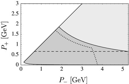
Figure 1: Relevant part of the phase space of semileptonic $B$ decays. The light-gray region denotes the portion where a background from $\bar{B}\to X_{c}\,l^{-}\bar{\nu}$ decays exists, while the dark-gray area is free of this background. Events with final-state hadronic invariant mass $M_{D}$ are located on the line between these two regimes. Events with $P_{+}\leq M_{D}^{2}/M_{B}$ are located below the dashed line. As a slightly more complicated example we also plot the borderline in phase space for events with $M_{X}\leq 1.7$ GeV and $q^{2}\geq 8$ GeV² as a dotted line.

In this paper, we extend the technology developed in [12] to derive the weight function for an arbitrary kinematic cut that includes events with $P_{+}\sim\Lambda_{\rm QCD}$ and $P_{-}\gg\Lambda_{\rm QCD}$. In general, the weight function $W(\Delta,P_{+})$ (and the correction $\Gamma_{\rm rhc}$), as well as the integration limit $\Delta$ in (1) depend on the particular cut that is used. For example, if we consider a cut on the charged-lepton energy $E_{l}\geq E_{0}$ then $\Delta=M_{B}-2E_{0}$, or if a cut on hadronic invariant mass $M_{X}\leq M_{0}$ is considered then one needs $\Delta=M_{0}$. A quick way to obtain some intuition on how $W(\Delta,P_{+})$ and $\Delta$ depend on the specific cut qualitatively is to consider the $\bar{B}\to X_{u}\,l^{-}\bar{\nu}$ phase-space depicted in Figure 1. Note that $P_{-}=M_{B}$ in radiative decays, so that the phase-space of $\bar{B}\to X_{s}\gamma$ consists only of the vertical boundary on the right-hand side of the plot. This picture explains correctly how the maximal $P_{+}^{\rm max}\equiv\Delta$ depends on the nature of the cut, and where to expect some kinks in $W(\Delta,P_{+})$, for example for a combined cut on $M_{X}$ and $q^{2}$.

In the next section we will derive an expression for the weight function at leading power, which follows from exact factorization theorems for differential rates in inclusive $B$ decays in the shape-function region. The formula for the weight function is thereby also valid to all orders in perturbation theory. We compute its explicit form to next-to-next-to leading order (NNLO) at the intermediate scale $\mu_{i}$ and to next-to leading order (NLO) at the hard scale $\mu_{h}$ in renormalization-group (RG) improved perturbation theory, including three-loop running effects. This approximation is sufficiently precise for phenomenological applications since effects at subleading power become as important as higher-order perturbative effects at leading power. In Section 3 we discuss first-order power corrections. Kinematical power corrections enter the weight function, while hadronic power corrections give rise the quantity $\Gamma_{\rm rhc}$ in (1). We then apply our results to a few examples of kinematic cuts in Section 4 and perform an analysis of theoretical uncertainties on $|V_{ub}|$ by using a simple model for the experimental inputs.

2 The weight function and factorization

In this section we will adopt the leading-power approximation. The second term on the right-hand side of relation (1) is then absent, because it collects contributions from subleading shape functions to both radiative and semileptonic decay rates, which start at order $1/m_{b}$.

2.1 Derivation

We start the discussion by stating the exact factorization theorems for the fully differential leading-power decay rate in $\bar{B}\to X_{u}\,l^{-}\bar{\nu}$ decays

$$\frac{d^{3}\Gamma_{u}^{(0)}}{dP_{+}\,dy\,d\varepsilon}= \;\frac{G_{F}^{2}|V_{ub}|^{2}}{192\pi^{3}}U(\mu_{h},\mu_{i})(M_{B}-P_{+})^{5}y^{-2a_{\Gamma}(\mu_{h},\mu_{i})}H_{u}(y,\varepsilon,\mu_{h})$$ (2)

$$\mbox{}\times\int_{0}^{P_{+}}d\hat{\omega}\;ym_{b}J(ym_{b}(P_{+}-\hat{\omega}),\mu_{i})\,\hat{S}(\hat{\omega},\mu_{i})\;,$$

and for the normalized $\bar{B}\to X_{s}\gamma$ photon spectrum

$$\frac{1}{\Gamma_{s}(E_{*})}\frac{d\Gamma_{s}^{(0)}}{dP_{+}}=\frac{U(\mu_{h},\mu_{i})}{H_{\Gamma}(E_{*},\mu_{h})}\frac{(M_{B}-P_{+})^{3}}{m_{b}^{3}}\int_{0}^{P_{+}}d\hat{\omega}\;m_{b}J(m_{b}(P_{+}-\hat{\omega}),\mu_{i})\,\hat{S}(\hat{\omega},\mu_{i})\;.$$ (3)

The superscript $(0)$ indicates that these equations are valid to leading power. In (2) $H_{u}(y,\varepsilon,\mu_{h})$ denotes the hard function, which collects all matching corrections at the scale $\mu_{h}$ and depends on the kinematic variables

$$y=\frac{P_{-}-P_{+}}{M_{B}-P_{+}}\;,\qquad\varepsilon=1-\frac{2E_{l}}{M_{B}-P_{+}}\;,$$ (4)

for which the phase-space is $0\leq\varepsilon\leq y\leq 1$. The jet function $J(p^{2},\mu_{i})$ contains distributions that act on the shape function $\hat{S}(\hat{\omega},\mu_{i})$ and depends on $y$ via $p^{2}=ym_{b}(P_{+}-\hat{\omega})$. In formula (3) for the photon spectrum, on the other hand, the hard function is denoted by $H_{\Gamma}(E_{*},\mu_{h})$, and the argument of the jet function is $p^{2}=m_{b}(P_{+}-\hat{\omega})$, independent of $y$ because $P_{-}=M_{B}$ in radiative decays. Three powers of the $b$-quark mass appear due to phase-space integrations in the total rate $\Gamma_{s}(E_{*})$. Renormalization-group (RG) running effects between the scales $\mu_{h}$ and $\mu_{i}$ build up the functions $U(\mu_{h},\mu_{i})$ and $a_{\Gamma}(\mu_{h},\mu_{i})$ in the factorization formulas, which are such that $U=1$ and $a_{\Gamma}=0$ in the limit $\mu_{i}\to\mu_{h}$. Expressions for them will be given below.

We start the derivation of the weight function by considering the factorized expression for an arbitrary partial differential decay rate

$$\Gamma_{u}^{(0)}\Big{|}_{\rm cut}=\int\limits_{0}^{\Delta}dP_{+}\int\limits_{0}^{y_{\rm max}[P_{+}]}dy\int\limits_{0}^{\varepsilon_{\rm max}[P_{+},y]}d\varepsilon\;\frac{d^{3}\Gamma_{u}^{(0)}}{dP_{+}\,dy\,d\varepsilon}\;.$$ (5)

The integration limits $y_{\rm max}[P_{+}]$ and $\varepsilon_{\rm max}[P_{+},y]$, as well as $\Delta$ depend on the specifics of the cut. (The use of squared brackets for these quantities is supposed to remind the reader that these functions are defined differently for different kinematic cuts.) We are now going to rewrite this semileptonic decay rate such that it resembles a weighted integral over the normalized photon spectrum. Clearly the biggest obstacle is that the argument of the jet function $J$ in (2) depends on the kinematic variable $y$, while it does not in (3). The solution to this problem has been presented in [12], where it was shown that a factorization of the integrated jet function in the sense that

$$j\left(\ln\frac{m_{b}\Omega}{\mu_{i}^{2}}+\ln y,\mu_{i}\right)=\int_{0}^{\Omega}dk\;Y(k,\ln y,\mu_{i})\;j\left(\ln\frac{m_{b}(\Omega-k)}{\mu_{i}^{2}},\mu_{i}\right)$$ (6)

can be achieved for arbitrary $\Omega$, if $Y(k,\ln y,\mu_{i})$ is allowed to be a distribution in the variable $k$. Here,

$$j\left(\ln\frac{Q^{2}}{\mu_{i}^{2}},\mu_{i}\right)\equiv\int_{0}^{Q^{2}}dp^{2}\,J(p^{2},\mu_{i})\;.$$ (7)

We will discuss the nature of $Y(k,\ln y,\mu_{i})$ and its perturbative expansion to two-loop order in the next section. The strategy for the derivation of the weight function is to interchange integrations in (5) so that the $P_{+}$ integration acts only on the jet function $J$, and we can make use of (6). Before this can be done, however, it is necessary to transform the other $P_{+}$-dependent terms in the partial decay rate into $P_{+}$-independent ones. This can be achieved by inserting

$$1=\int_{0}^{\Delta}dP^{\prime}\;\delta(P^{\prime}-P_{+})=\int_{0}^{\Delta}dP^{\prime}\int_{0}^{M_{B}-P_{+}}dq\;\delta^{\prime}(q+P^{\prime}-M_{B})\;,$$ (8)

into (5), and by replacing $P_{+}\to P^{\prime}$ in $y_{\rm max}[P_{+}]$, $\varepsilon_{\rm max}[P_{+}]$ and in the kinematic prefactor $(M_{B}-P_{+})^{5}$. It is now an easy exercise to interchange the integrations

$$\int\limits_{0}^{\Delta}dP_{+}\int\limits_{0}^{P_{+}}d\hat{\omega}\int\limits_{0}^{M_{B}-P_{+}}dq\ldots=\int\limits_{0}^{\Delta}d\hat{\omega}\int\limits_{0}^{M_{B}-\hat{\omega}}dq\int\limits_{\hat{\omega}}^{{\rm min}(\Delta,M_{B}-q)}dP_{+}\ldots\;.$$ (9)

Next, we apply (6), interchange the $k$ and $P_{+}$ integrations, and undo the steps in (9). Finally the integrations over $q$ and $P^{\prime}$ can be carried out, which identifies $P^{\prime}=P_{+}+k$. As a result we arrive at an expression for the semileptonic decay rate, which is given as an integral over the product of the normalized photon spectrum in (3) and

$$W^{(0)}(\Delta,P_{+})=\frac{G_{F}^{2}\,H_{\Gamma}(\mu_{h})}{192\pi^{3}}\frac{m_{b}^{3}}{(M_{B}-P_{+})^{3}}\int\limits_{0}^{\Delta-P_{+}}dk\;F(P_{+}+k,k,\mu_{h},\mu_{i})\;,$$ (10)

where

$$F(P^{\prime},k,\mu_{h},\mu_{i})=(M_{B}-P^{\prime})^{5}\int\limits_{0}^{y_{\rm max}[P^{\prime}]}dy\int\limits_{0}^{\varepsilon_{\rm max}[P^{\prime},y]}d\varepsilon\;y^{-2a_{\Gamma}(\mu_{h},\mu_{i})}H_{u}(y,\varepsilon,\mu_{h})\,Y(k,\ln y,\mu_{i})\;.$$ (11)

The above two formulas enable us to calculate the weight function in an automated fashion. The procedure is as follows: first, the integration limits $\Delta$, $y_{\rm max}[P_{+}]$, and $\varepsilon_{\rm max}[P_{+}]$ are specified from the kinematics of the cut. For the next step it is helpful to decompose $Y(k,\ln y,\mu_{i})=\sum_{i}{\cal D}_{i}(k,\mu_{i})\,Y_{i}(\ln y,\mu_{i})$, where ${\cal D}_{i}(k,\mu_{i})$ are distributions in $k$ and independent of $y$. (For example, we will see below that there are only three different distributions in the perturbative expansion of $Y(k,\ln y,\mu_{i})$ to two-loop order.) Likewise, we decompose $F(P^{\prime},k,\mu_{h},\mu_{i})=\sum_{i}{\cal D}_{i}(k,\mu_{i})\,F_{i}(P^{\prime},\mu_{h},\mu_{i})$. It is then straight-forward to calculate the functions $F_{i}(P^{\prime},\mu_{h},\mu_{i})$ by integrating over $\varepsilon$ and $y$ in (11). Finally the integration over $k$ is performed in (10), where the distributions ${\cal D}_{i}(k,\mu_{i})$ act on $F_{i}(P_{+}+k,\mu_{h},\mu_{i})$.

Equation (10) together with (6) is the main result of this paper. We stress that both formulas are exact factorization theorems (in the convolution sense), valid to all orders in perturbation theory, and (10) gives the exact leading-power weight function for arbitrary cuts.

2.2 Perturbative calculation

The computation of the kernel $Y(k,\ln y,\mu)$ in (6) requires the knowledge of the jet integral $j(L,\mu)$. The jet function $J(p^{2},\mu_{i})$ has been calculated to one-loop order explicitly [4, 5], and the non-constant part of $j(L,\mu)$ at two-loop order can be extracted from RG evolution [7]. Because the jet integral is of central importance to the present work, we find it legitimate to re-derive its dependence on $L$ in detail. In particular, from the RG equations for the shape function and the leading-power current in soft-collinear effective theory (SCET, see also [13]),

$$0 = \int_{0}^{\hat{\omega}}d\hat{\omega}^{\prime}\left\{\left[\frac{d}{d\ln\mu}+2\gamma_{S}(\mu)\right]\delta(\hat{\omega}-\hat{\omega}^{\prime})-2\Gamma_{c}(\mu)\left(\frac{1}{\hat{\omega}-\hat{\omega}^{\prime}}\right)_{*}^{[\mu]}\right\}\hat{S}(\hat{\omega},\mu)\;,$$ (12)

$$0 = \left[\frac{d}{d\ln\mu}+2\gamma^{\prime}(\mu)+2\Gamma_{c}(\mu)\ln\frac{m_{b}}{\mu}\right]\int_{0}^{P_{+}}d\hat{\omega}\;m_{b}J(m_{b}(P_{+}-\hat{\omega}),\mu)\;\hat{S}(\hat{\omega},\mu)\;,$$

we can derive the RG equation governing $j(L,\mu)$ with $L=\ln Q^{2}/\mu^{2}$ and arbitrary $Q^{2}$. Above, $\Gamma_{c}(\mu)$ is the cusp anomalous dimension [14], which has been calculated to three-loop order [15], the remaining anomalous dimensions $\gamma_{S}(\mu)$ and $\gamma^{\prime}(\mu)$ are known to two-loop order [6, 16, 17]. (For a definition of the star distribution that acts on the shape function see (16) below.) When combining the two RG equations, one finds

$$\frac{d}{d\ln\mu}j(L,\mu)=-2\left[\Gamma_{c}(\mu)L+\gamma^{J}(\mu)\right]j(L,\mu)-2\Gamma_{c}\int_{0}^{1}\frac{dz}{z}\big{[}j(L+\ln(1-z),\mu)-j(L,\mu)\big{]},$$ (13)

with $\gamma^{J}=\gamma^{\prime}-\gamma_{S}$. This integro-differential equation can be solved perturbatively by choosing a polynomial ansatz for $j(L,\mu)$. As a result the integral in the above equation leads to the appearance of the Riemann zeta-function $\zeta_{n}$. Specifically, after expanding the QCD $\beta$-function and anomalous dimensions as

$$\beta(\mu)=\frac{d\alpha_{s}(\mu)}{d\ln\mu}=-2\alpha_{s}(\mu)\sum\limits_{n=0}^{\infty}\beta_{n}\left(\frac{\alpha_{s}(\mu)}{4\pi}\right)^{n+1}\;,\quad\Gamma_{c}(\mu)=\sum\limits_{n=0}^{\infty}\Gamma_{n}\left(\frac{\alpha_{s}(\mu)}{4\pi}\right)^{n+1}\;,$$ (14)

and similarly $\gamma^{J}(\mu)$, we find to two-loop accuracy

$$j(L,\mu) = 1+\frac{\alpha_{s}(\mu)}{4\pi}\left[b_{0}^{(1)}+\gamma_{0}^{J}L+\frac{1}{2}\Gamma_{0}L^{2}\right]$$

$$\mbox{}+\left(\frac{\alpha_{s}(\mu)}{4\pi}\right)^{2}\Bigg{[}b_{0}^{(2)}+\left(b_{0}^{(1)}(\gamma_{0}^{J}-\beta_{0})+\gamma_{1}^{J}-\frac{\pi^{2}}{6}\Gamma_{0}\gamma_{0}^{J}+\zeta_{3}\Gamma_{0}^{2}\right)L$$

$$\mbox{}+\frac{1}{2}\left(\gamma_{0}^{J}(\gamma_{0}^{J}-\beta_{0})+b_{0}^{(1)}\Gamma_{0}+\Gamma_{1}-\frac{\pi^{2}}{6}\Gamma_{0}^{2}\right)L^{2}-\left(\frac{1}{6}\beta_{0}-\frac{1}{2}\gamma_{0}^{J}\right)\Gamma_{0}L^{3}+\frac{1}{8}\Gamma_{0}^{2}L^{4}\Bigg{]}.$$

Here, $b_{0}^{(1)}=C_{F}(7-\pi^{2})$ is the one-loop constant, and the two-loop constant $b_{0}^{(2)}$ is currently unknown. To determine it a multi-loop calculation will be necessary. However, this constant does not enter the two-loop result for the kernel $Y(k,\ln y,\mu_{i})$.

Next, we need to find an ansatz for $Y(k,\ln y,\mu)$ which satisfies (6). At tree-level $j(L,\mu)=1$ and therefore $Y(k,\ln y,\mu)=\delta(k)$ is also independent of $y$. It follows that the constant $b_{0}^{(2)}$ cancels in the relation (6) to two-loop accuracy. Beyond the tree approximation the integrated $Y(k,\ln y,\mu)$ (defined equivalently to (7)) must pick up a logarithmic dependence on $\Omega$, as can be seen by interchanging the integrations in (6); but $Y(k,\ln y,\mu)$ itself must not depend on $\Omega$. Objects that accomplish that are already known from the jet function $J(p^{2},\mu)$, and are called “star-distributions” [18] (see also [4, 5, 8]). Their definitions are such that, when integrated over an interval $\Omega$, they act on a function $\phi(k)$ as

$$\int_{0}^{\Omega}dk\,\left(\frac{1}{k}\right)_{*}^{[\mu^{2}/m_{b}]}\phi(k) = \int_{0}^{\Omega}dk\,\frac{\phi(k)-\phi(0)}{k}\,+\phi(0)\,\ln\frac{m_{b}\Omega}{\mu^{2}}\,,$$ (16)

$$\int_{0}^{\Omega}dk\,\left(\frac{1}{k}\ln\frac{m_{b}k}{\mu^{2}}\right)_{*}^{[\mu^{2}/m_{b}]}\phi(k) = \int_{0}^{\Omega}dk\,\frac{\phi(k)-\phi(0)}{k}\ln\frac{m_{b}k}{\mu_{i}^{2}}\,+\frac{\phi(0)}{2}\,\ln^{2}\frac{m_{b}\Omega}{\mu^{2}}\,.$$

Therefore, the ansatz for the jet kernel reads (here with $L=\ln y$ for brevity)

$$Y(k,L,\mu) = \delta(k)+\frac{\alpha_{s}(\mu)}{4\pi}\left[c_{0}^{(1)}(L)\,\delta(k)+c_{1}^{(1)}(L)\left(\frac{1}{k}\right)^{[\mu^{2}/m_{b}]}_{*}\right]$$

$$\mbox{}+\left(\frac{\alpha_{s}(\mu)}{4\pi}\right)^{2}\left[c_{0}^{(2)}(L)\,\delta(k)+c_{1}^{(2)}(L)\left(\frac{1}{k}\right)^{[\mu^{2}/m_{b}]}_{*}+c_{2}^{(2)}(L)\left(\frac{1}{k}\ln\frac{m_{b}k}{\mu^{2}}\right)^{[\mu^{2}/m_{b}]}_{*}\right].$$

In (10) it acts on all $k$-dependent objects, i.e., on the prefactor $(M_{B}-P_{+}-k)^{2}$ and on the integration limits $y_{\rm max}[P_{+}+k]$ and $\varepsilon_{\rm max}[P_{+}+k,y]$. To determine the coefficients $c^{(n)}_{i}(L)$, however, we consult (6), where the star distributions act on the $k$-dependent logarithms. We find

$$c^{(1)}_{1}(L) = \Gamma_{0}L\;,\quad c^{(1)}_{0}(L)=\gamma^{J}_{0}L+\frac{\Gamma_{0}}{2}L^{2}\;,$$ (18)

$$c^{(2)}_{2}(L) = -\Gamma_{0}L(\beta_{0}-\Gamma_{0}L)\;,\quad c^{(2)}_{1}(L)=\left[\Gamma_{1}-\beta_{0}\gamma^{J}_{0}\right]L+\left[\Gamma_{0}\gamma^{J}_{0}-\beta_{0}\frac{\Gamma_{0}}{2}\right]L^{2}+\frac{\Gamma_{0}^{2}}{2}L^{3}\;,$$

$$c^{(2)}_{0}(L) = \left[\gamma^{J}_{1}-b^{(1)}_{0}\beta_{0}\right]L+\left[\frac{\gamma^{J}_{0}}{2}(\gamma^{J}_{0}-\beta_{0})+\frac{\Gamma_{1}}{2}-\frac{\pi^{2}}{12}\Gamma_{0}^{2}\right]L^{2}+\frac{\Gamma_{0}}{2}\left[\gamma^{J}_{0}-\frac{1}{3}\beta_{0}\right]L^{3}+\frac{\Gamma_{0}^{2}}{8}L^{4}\;.$$

At this point we interrupt the discussion briefly and consider the result for the weight function in (10) again. As mentioned earlier, the $b$-quark mass enters the normalization of the weight function since we also normalized the photon spectrum. In order to avoid the renormalon ambiguities of the pole scheme it is favorable to use a low-scale subtracted quark-mass definition, for which we adopt the shape-function scheme [5]. The two mass definitions are connected via

$$m_{b}^{\rm pole}=m_{b}^{\rm SF}(\mu_{*})+\mu_{*}\frac{C_{F}\alpha_{s}(\mu_{h})}{\pi}+\ldots\;,$$ (19)

and we will refer to $m_{b}^{\rm SF}(\mu_{*})$ at $\mu_{*}=1.5$ GeV as $m_{b}$ for brevity, for the rest of this paper. Apart from the normalization to the weight function, $m_{b}$ also enters through radiative logarithms in the hard functions and through star distributions in the jet kernel. Since the hard functions are only kept to one-loop order, the above redefinition of $m_{b}$ does not affect the result. $Y(k,\ln y,\mu_{i})$, on the other hand, is given to two-loop accuracy in (2.2). It follows that $c_{0}^{(1)}$ receives a contribution at this level,

$$c^{(1)}_{0}(L)=\left[\gamma_{0}+\frac{C_{F}\alpha_{s}(\mu_{h})}{\pi}\frac{\mu_{*}}{m_{b}}\Gamma_{0}\right]L+\frac{\Gamma_{0}}{2}L^{2}\;.$$ (20)

In the remainder of this section we collect the other ingredients of (10) for completeness. The hard function in semileptonic decays is known to 1-loop order in perturbation theory and given by

$$H_{u}(y,\varepsilon,\mu_{h})= \;12(y-\varepsilon)(1-y+\varepsilon)\bigg{\{}1+\frac{C_{F}\alpha_{s}(\mu_{h})}{4\pi}\Big{[}-4\ln^{2}\frac{ym_{b}}{\mu_{h}}+10\ln\frac{ym_{b}}{\mu_{h}}-4\ln y$$ (21)

$$\mbox{}\hskip 85.35826pt-4L_{2}(1-y)-\frac{\pi^{2}}{6}-12\Big{]}\bigg{\}}-6(y-\varepsilon)\frac{C_{F}\alpha_{s}(\mu_{h})}{\pi}\ln y\;.$$

The hard function for the normalized photon spectrum reads

$$H_{\Gamma}(\mu_{h}) = 1+\frac{C_{F}\alpha_{s}(\mu_{h})}{4\pi}\Bigg{\{}4\ln^{2}\frac{m_{b}}{\mu_{h}}-10\ln\frac{m_{b}}{\mu_{h}}+7-\frac{7\pi^{2}}{6}+12\frac{\mu_{*}}{m_{b}}$$ (22)

$$\mbox{}-2\ln^{2}\delta_{*}-(7+4\delta_{*}-\delta_{*}^{2})\ln\delta_{*}+10\delta_{*}+\delta_{*}^{2}-\frac{2}{3}\delta_{*}^{3}$$

$$\mbox{}+\frac{[C_{1}(\mu_{h})]^{2}}{[C^{\rm eff}_{7\gamma}(\mu_{h})]^{2}}\,\hat{f}_{11}(\delta_{*})+\frac{C_{1}(\mu_{h})}{C^{\rm eff}_{7\gamma}(\mu_{h})}\hat{f}_{17}(\delta_{*})+\frac{C_{1}(\mu_{h})\,C_{8g}^{\rm eff}(\mu_{h})}{[C^{\rm eff}_{7\gamma}(\mu_{h})]^{2}}\hat{f}_{18}(\delta_{*})$$

$$\mbox{}+\frac{C_{8g}^{\rm eff}(\mu_{h})}{C^{\rm eff}_{7\gamma}(\mu_{h})}\hat{f}_{78}(\delta_{*})+\frac{[C_{8g}^{\rm eff}(\mu_{h})]^{2}}{[C^{\rm eff}_{7\gamma}(\mu_{h})]^{2}}\hat{f}_{88}(\delta_{*})\Bigg{\}}.$$

Here, $\delta_{*}=1-2E_{*}/m_{b}=0.9$, and the functions $\hat{f}_{ij}(\delta_{*})$ capture effects from operator mixing [19] and can be found in this notation in [6]. Note also the term proportional to $\alpha_{s}(\mu_{h})\,\mu_{*}/m_{b}$, which ensures that the three powers of $m_{b}$ in (10) are defined in the shape-function scheme. Finally, the RG function $a_{\Gamma}$ is defined as the integrated cusp anomalous dimension from $\ln\mu_{i}$ to $\ln\mu_{h}$, which yields

$$a_{\Gamma}(\mu_{h},\mu_{i}) = \frac{\Gamma_{0}}{2\beta_{0}}\,\Bigg{\{}\ln\frac{\alpha_{s}(\mu_{i})}{\alpha_{s}(\mu_{h})}+\frac{\alpha_{s}(\mu_{i})-\alpha_{s}(\mu_{h})}{4\pi}\left[\frac{\Gamma_{1}}{\Gamma_{0}}-\frac{\beta_{1}}{\beta_{0}}\right]$$ (23)

$$\mbox{}+\frac{\alpha_{s}^{2}(\mu_{i})-\alpha_{s}^{2}(\mu_{h})}{32\pi^{2}}\left[\frac{\beta_{1}}{\beta_{0}}\left(\frac{\beta_{1}}{\beta_{0}}-\frac{\Gamma_{1}}{\Gamma_{0}}\right)-\frac{\beta_{2}}{\beta_{0}}+\frac{\Gamma_{2}}{\Gamma_{0}}\right]+\dots\Bigg{\}}.$$

When combining the various quantities into (10) the result should be re-expanded in $\alpha_{s}$ to the order in which we are working. However, it is convenient to treat $a_{\Gamma}(\mu_{h},\mu_{i})$ as a running “physical” quantity (similar to $\alpha_{s}(\mu)$), which is not expanded. This is the same approach as put forward in [12], and we will use it in the phenomenological applications in Section 4.

Expansion coefficients of the anomalous dimensions.

To three-loop order, the coefficients of the $\beta$ function read [20]

$$\beta_{0} = \frac{11}{3}\,C_{A}-\frac{2}{3}\,n_{f}\,,\qquad\beta_{1}=\frac{34}{3}\,C_{A}^{2}-\frac{10}{3}\,C_{A}\,n_{f}-2C_{F}\,n_{f}\,,$$ (24)

$$\beta_{2} = \frac{2857}{54}\,C_{A}^{3}+\left(C_{F}^{2}-\frac{205}{18}\,C_{F}C_{A}-\frac{1415}{54}\,C_{A}^{2}\right)n_{f}+\left(\frac{11}{9}\,C_{F}+\frac{79}{54}\,C_{A}\right)n_{f}^{2}\,,$$

where $n_{f}=4$ is the number of light flavors, $C_{A}=3$ and $C_{F}=4/3$. The cusp anomalous dimension to three-loop order is given by [14, 15]

$$\Gamma_{0} = 4C_{F}\,,\qquad\Gamma_{1}=8C_{F}\left[\left(\frac{67}{18}-\frac{\pi^{2}}{6}\right)C_{A}-\frac{5}{9}\,n_{f}\right],$$ (25)

$$\Gamma_{2} = 16C_{F}\bigg{[}\left(\frac{245}{24}-\frac{67\pi^{2}}{54}+\frac{11\pi^{4}}{180}+\frac{11}{6}\,\zeta_{3}\right)C_{A}^{2}+\left(-\frac{209}{108}+\frac{5\pi^{2}}{27}-\frac{7}{3}\,\zeta_{3}\right)C_{A}\,n_{f}$$

$$\mbox{}\qquad+\left(-\frac{55}{24}+2\zeta_{3}\right)C_{F}\,n_{f}-\frac{1}{27}\,n_{f}^{2}\bigg{]}.$$

We also need the anomalous dimension coefficients for the integrated jet function $j(L,\mu)$, which are [6]

$$\gamma_{0}^{J} = -3C_{F}$$ (26)

$$\gamma_{1}^{J} = C_{F}\left[-\left(\frac{3}{2}-2\pi^{2}+24\zeta_{3}\right)C_{F}-\left(\frac{1769}{54}+\frac{11}{9}\pi^{2}-40\zeta_{3}\right)C_{A}+\left(\frac{121}{27}+\frac{2}{9}\pi^{2}\right)n_{f}\right].$$

3 Power corrections

Factorization theorems exist at each level of power counting for differential decay rates in inclusive heavy-quark decays. We differentiate between two types of power corrections, “kinematical” and “hadronic”. The first class arises simply because we have restricted our discussion to a particular portion in phase-space, where $P_{+}\ll M_{B}$. These corrections are power suppressed in the shape-function region, but are of leading power when integrated over a domain that is comparable to $M_{B}$ (OPE region). A different way of thinking about kinematical corrections is to view them as the equivalent of the factorization theorems (2) and (3) with subleading hard and jet functions. However, no complete scale separation has been achieved for these power corrections yet, but the products of subleading hard and jet functions are known in fixed-order perturbation theory and to all powers from [18, 19]. Since kinematical corrections start at $\alpha_{s}(\bar{\mu})$ and are numerically small for all prominent cuts, this approximate treatment suffices. The scale $\bar{\mu}$ is typically near $\sqrt{m_{b}\Lambda_{\rm QCD}}$, but independent of $\mu_{i}$ and $\mu_{h}$.

The second class of corrections comes from subleading hadronic structure functions [21, 22, 23, 24, 25, 26, 27, 28]. Already at first subleading order there are multiple independent shape functions entering the calculation of the differential decay rates. Furthermore, they appear in different linear combinations in the semileptonic and radiative cases, so that at this stage a weight function cannot relate semileptonic decay rates to radiative ones alone. In equation (1) we have therefore added a second term labeled $\Gamma_{\rm rhc}$. Note that this term is different from the subleading shape-function contribution to the semileptonic decay rate (denoted $\Gamma_{u}^{\rm hadr}$ in [8]) since contributions from subleading hadronic corrections to the photon spectrum are convoluted with the leading-power weight function and must be subtracted. As a result the residual hadronic power corrections are collected in $\Gamma_{\rm rhc}$. Currently the hard and jet functions in the subleading shape-function contributions to the decay rates are only known at tree-level.

3.1 Kinematical corrections

Since kinematical corrections come with the leading shape function, the corresponding contribution to the weight function $W^{\rm kin}(\Delta,P_{+})$ can be calculated without the introduction of any hadronic uncertainty. These terms start at order $\alpha_{s}(\bar{\mu})$ and we only compute the correction to this order. It thus follows that $W^{\rm kin}\otimes d\Gamma_{s}^{(0)}=\Gamma_{u}^{\rm kin}-W^{(0)}\otimes d\Gamma_{s}^{\rm kin}$, symbolically. (Here and below the abbreviation $d\Gamma_{s}$ in statements within the main text denotes the normalized photon spectrum.) The relevant expressions for the differential decay rates have been collected in [8] and may be written as (here and below $a_{\Gamma}=a_{\Gamma}(\mu_{h},\mu_{i})$ for brevity)

$$\Gamma_{u}^{\rm kin}\Big{|}_{\rm cut} = N_{u}\int\limits_{0}^{\Delta}dP_{+}\int\limits_{0}^{y_{\rm max}[P_{+}]}dy\int\limits_{0}^{\varepsilon_{\rm max}[P_{+},y]}d\varepsilon\;y^{-2a_{\Gamma}}(M_{B}-P_{+})^{4}\int\limits_{0}^{P_{+}}d\hat{\omega}\;K_{u}(x,y,\varepsilon)\,\hat{S}(\hat{\omega})\;,$$

$$\frac{1}{\Gamma_{s}}\frac{d\Gamma_{s}^{\rm kin}}{dP_{+}} = N_{s}\frac{(M_{B}-P_{+})^{2}}{m_{b}^{3}}\int\limits_{0}^{P_{+}}d\hat{\omega}\;K_{s}(x)\,\hat{S}(\hat{\omega})\;,\qquad\hbox{with}\;\;x=\frac{P_{+}-\hat{\omega}}{M_{B}-P_{+}}\;,$$ (27)

where we have collected all terms in the functions $K_{u}(\varepsilon,y,x)$ and $K_{s}(x)$, and abbreviated the different norms by $N_{u}$ and $N_{s}$. The leading weight function at tree-level is taken from (10). We now transform the expression for $\Gamma_{u}^{\rm kin}-W^{(0)}\otimes d\Gamma_{s}^{\rm kin}$ in three steps: First, we interchange the order of the $P_{+}$ and $\hat{\omega}$ integrations. Next, the integration variable $P_{+}$ is substituted by $k=P_{+}-\hat{\omega}$. Finally the variable $\hat{\omega}$ is renamed by $P_{+}$. After this has been done (no manipulation is needed for the term $W^{\rm kin}\otimes d\Gamma_{s}^{(0)}$), we find

$$W^{\rm kin}(\Delta,P_{+}) = \frac{N_{u}}{N_{s}}\frac{m_{b}^{3}}{(M_{B}-P_{+})^{3}}\int\limits_{0}^{\Delta-P_{+}}dk\;(M_{B}-P_{+}-k)^{4}\int\limits_{0}^{y_{\rm max}[P_{+}+k]}dy\int\limits_{0}^{\varepsilon_{\rm max}[P_{+}+k,y]}d\varepsilon\;y^{-2a_{\Gamma}}$$ (28)

$$\mbox{}\times\left[K_{u}\left(\frac{k}{M_{B}-P_{+}-k},y,\varepsilon\right)-H_{u}^{(0)}(y,\varepsilon)\,K_{s}\left(\frac{k}{M_{B}-P_{+}-k}\right)\right],$$

where $H_{u}^{(0)}(y,\varepsilon)$ denotes the tree-level part of the hard function in (21).

We are now going to restrict the calculation to the first-order power corrections because of mixing effects with hadronic power corrections at higher orders. For example, the second-order power correction to the weighted integral over the photon spectrum contains a term $W^{\rm kin(1)}\otimes d\Gamma_{s}^{\rm hadr(1)}$. (As before, the superscript denotes the order in power counting.) For such a term we would require a compensation in the residual correction $\Gamma_{\rm rhc}$ at order $\alpha_{s}(\bar{\mu})$, which goes beyond the scope of this paper. Including only first-order power corrections is not a bad approximation; the studies in [8] have shown that the full kinematical corrections can be approximated very well by including the first term in the power expansion only. At this level the functions $K_{u}(x,y,\varepsilon)$ and $K_{s}(x)$ involve only two different functional dependences on $x$, a constant and a term proportional to $\ln x$. We find

$$W^{\rm(kin,1)}(\Delta,P_{+})= \frac{G_{F}^{2}}{192\pi^{3}}\frac{m_{b}^{3}}{(M_{B}-P_{+})^{3}}\frac{C_{F}\alpha_{s}(\bar{\mu})}{4\pi}\int\limits_{0}^{\Delta-P_{+}}dk\;(M_{B}-P_{+}-k)^{4}$$ (29)

$$\mbox{}\times\int\limits_{0}^{y_{\rm max}[P_{+}+k]}dy\int\limits_{0}^{\varepsilon_{\rm max}[P_{+}+k,y]}d\varepsilon\;y^{-2a_{\Gamma}}\left[A(y,\varepsilon)+B(y,\varepsilon)\ln\frac{k}{M_{B}-P_{+}-k}\right]$$

with

$$A(y,\varepsilon) = 12\Bigg{[}\frac{\varepsilon(5+27\varepsilon)}{y}-4-53\varepsilon-25\varepsilon^{2}+y(25+46\varepsilon)-21y^{2}$$

$$\mbox{}+4\,\frac{y-\varepsilon}{y}\left[3+5\varepsilon-(4+\varepsilon)y+y^{2}\right]\ln y\Bigg{]}$$

$$\mbox{}+12(y-\varepsilon)(1-y+\varepsilon)\Bigg{[}\left(\frac{1}{3}-\frac{4}{9}\ln\frac{m_{b}}{m_{s}}\right)\frac{[C_{8g}^{\rm eff}(\mu_{h})]^{2}}{[C_{7\gamma}^{\rm eff}(\mu_{h})]^{2}}-\frac{10}{3}\frac{C_{8g}^{\rm eff}(\mu_{h})}{C_{7\gamma}^{\rm eff}(\mu_{h})}$$

$$\mbox{}+\frac{8}{3}\left(\frac{C_{1}(\mu_{h})}{C_{7\gamma}^{\rm eff}(\mu_{h})}-\frac{1}{3}\frac{C_{1}(\mu_{h})C_{8g}^{\rm eff}(\mu_{h})}{[C_{7\gamma}^{\rm eff}(\mu_{h})]^{2}}\right)\,g_{1}(z)-\frac{16}{9}\,\frac{[C_{1}(\mu_{h})]^{2}}{[C_{7\gamma}^{\rm eff}(\mu_{h})]^{2}}\,g_{2}(z)\Bigg{]},$$

$$B(y,\varepsilon) = 48\,\frac{y-\varepsilon}{y}(1-y)(-3+5y-5\varepsilon)-\frac{8}{3}(1-y+\varepsilon)(y-\varepsilon)\frac{[C_{8g}^{\rm eff}(\mu_{h})]^{2}}{[C_{7\gamma}^{\rm eff}(\mu_{h})]^{2}}\;.$$

In these expressions $C_{i}(\mu_{h})$ denote the (effective) Wilson coefficients of the relevant operators in the effective weak Hamiltonian for $\bar{B}\to X_{s}\gamma$ decay. Charm-loop penguin contributions to the hard function of the photon spectrum are encoded in the functions $g_{1}(z)$ and $g_{2}(z)$, which depend on the variable $z=(m_{c}/m_{b})^{2}$ [19]. They are

$$g_{1}(z)=\int_{0}^{1}dx\,x\,\mbox{Re}\left[\,\frac{z}{x}\,G\left(\frac{x}{z}\right)+\frac{1}{2}\,\right],\\$$

$$g_{2}(z) = \int_{0}^{1}dx\,(1-x)\left|\,\frac{z}{x}\,G\left(\frac{x}{z}\right)+\frac{1}{2}\,\right|^{2}\,,$$ (30)

$$G(t) = \left\{\begin{array}[]{ll}-2\arctan^{2}\sqrt{t/(4-t)}&~{};~{}t<4\,,\\[2.84544pt] 2\left(\ln\Big{[}(\sqrt{t}+\sqrt{t-4})/2\Big{]}-\displaystyle\frac{i\pi}{2}\right)^{2}&~{};~{}t\geq 4\,.\end{array}\right.$$ (33)

This concludes the calculation of the weight function.

3.2 Residual hadronic corrections

There are four different hadronic structures entering the first-order power corrections to the differential decay rates at tree level. Following [27] we denote them by $(\bar{\Lambda}-\hat{\omega})\hat{S}(\hat{\omega})$, $\hat{t}(\hat{\omega})$, $\hat{u}(\hat{\omega})$, and $\hat{v}(\hat{\omega})$. The first one in this list involves the leading shape function and the heavy-quark parameter $\bar{\Lambda}$. This parameter ensures that $(\bar{\Lambda}-\hat{\omega})\hat{S}(\hat{\omega})$ has a vanishing norm, as all subleading shape functions must have. It is possible to absorb the effect of this function into a weight-function contribution, which in turn only depends on $(\bar{\Lambda}-P_{+})$; however, because of the zero-norm constraint it is difficult to assign the correct numerical value of $\bar{\Lambda}$ in that case. Instead, we keep this contribution together with the subleading shape functions in $\Gamma_{\rm rhc}$. A straight-forward calculation yields

$$\Gamma_{\rm rhc}\Big{|}_{\rm cut} = \frac{G_{F}^{2}\,U(\mu_{h},\mu_{i})}{16\pi^{3}}\int_{0}^{\Delta}dP_{+}\;(M_{B}-P_{+})^{4}\int\limits_{0}^{y_{\rm max}[P_{+}]}dy\int\limits_{0}^{\varepsilon_{\rm max}[P_{+},y]}d\varepsilon\;y^{-2a_{\Gamma}}\;\frac{y-\varepsilon}{y}$$

$$\mbox{}\times\Bigg{\{}2(1-y)(y-\varepsilon)\;(\bar{\Lambda}-P_{+})\hat{S}(P_{+})+2(1-y)\left(y-\varepsilon+\frac{\varepsilon}{y}\right)\hat{t}(P_{+})$$

$$\mbox{}\quad+(1-y)(1-y+\varepsilon)\,\hat{u}(P_{+})+\left(1+y-\frac{y-\varepsilon}{y}(2-y+y^{2})\right)\hat{v}(P_{+})$$

$$\mbox{}\quad+y(1-y+\varepsilon)\,m_{s}^{2}\hat{S}^{\prime}(P_{+})\Bigg{\}},$$

where we have kept the RG-evolution function $y^{-2a_{\Gamma}}$, as well as $U(\mu_{h},\mu_{i})$ [8]. Its structure is such that

$$\ln U(\mu_{h},\mu_{i})=2S_{\Gamma}(\mu_{h},\mu_{i})-2a_{\Gamma}(\mu_{h},\mu_{i})\ln\frac{m_{b}}{\mu_{h}}-2a_{\gamma^{\prime}}(\mu_{h},\mu_{i})\;,$$ (35)

and we evaluate to leading-order the Sudakov exponent (with $r=\alpha_{s}(\mu_{i})/\alpha_{s}(\mu_{h})$)

$$S_{\Gamma}(\mu_{h},\mu_{i})=\frac{\Gamma_{0}}{4\beta_{0}^{2}}\,\left\{\frac{4\pi}{\alpha_{s}(\mu_{h})}\left(1-\frac{1}{r}-\ln r\right)+\left(\frac{\Gamma_{1}}{\Gamma_{0}}-\frac{\beta_{1}}{\beta_{0}}\right)(1-r+\ln r)+\frac{\beta_{1}}{2\beta_{0}}\ln^{2}r\right\},$$ (36)

and the RG function $a_{\gamma^{\prime}}=\gamma^{\prime}_{0}/(2\beta_{0})\,\ln r$ analogous to (23). The use of the anomalous dimension $\gamma^{\prime}_{0}=-5C_{F}$ of the leading SCET current is a good approximation because most of the subleading operators in SCET are build from the leading SCET current and thus share the same anomalous dimension. (A complete resummation requires knowledge of the anomalous dimension matrix of all subleading operators in SCET. For some discussion, see e.g. [29, 30, 31].)

We have included a small correction from a finite $s$-quark mass, leading to the expression proportional to $m_{s}^{2}S^{\prime}(P_{+})$. The appearance of hadronic structure functions in (3.2) introduces some irreducible uncertainties in phenomenological applications of our results. While in principle the leading shape function $\hat{S}(\hat{\omega})$ can be extracted from the photon spectrum, see e.g. [8], the forms of the shape functions $\hat{t}(\hat{\omega})$, $\hat{u}(\hat{\omega})$, and $\hat{v}(\hat{\omega})$ are unknown. What we know is that their norms vanish and their first moments are given in terms of the heavy-quark parameters $\mu_{\pi}^{2}$ and $\lambda_{2}$. In order to estimate effects from higher moments we define functions $h_{n}(\hat{\omega})$, $n\in\{t,u,v\}$, via

$$\hat{t}(\hat{\omega})=-\lambda_{2}\;\hat{S}^{\prime}(\hat{\omega})+h_{t}(\hat{\omega})\;,\quad\hat{u}(\hat{\omega})=-2\;\frac{\mu_{\pi}^{2}}{3}\;\hat{S}^{\prime}(\hat{\omega})+h_{u}(\hat{\omega})\;,\quad\hat{v}(\hat{\omega})=\lambda_{2}\;\hat{S}^{\prime}(\hat{\omega})+h_{v}(\hat{\omega})\;.$$ (37)

As long as each of the $h_{n}(\hat{\omega})$ have zero norm and first moment the constraints on the subleading shape functions are satisfied.

Let us now adopt a default model for the terms in (3.2). For simplicity we use for $\hat{S}(\hat{\omega})$ the familiar exponential-type functional form

$$\hat{S}(\hat{\omega})=\frac{1}{\bar{\Lambda}}\frac{b^{b}}{\Gamma(b)}\left(\frac{\hat{\omega}}{\bar{\Lambda}}\right)^{b-1}\exp\left(-b\,\frac{\hat{\omega}}{\bar{\Lambda}}\right),\qquad\hbox{with}\quad b=\frac{3\bar{\Lambda}^{2}}{\mu_{\pi}^{2}}\;,$$ (38)

with parameters $\bar{\Lambda}$ and $\mu_{\pi}^{2}$. By construction the moment constraints on $(\bar{\Lambda}-\hat{\omega})\hat{S}(\hat{\omega})$ are respected. The default model for (37) is defined as $h_{n}(\hat{\omega})=0$ in all three cases.

In order to estimate the uncertainty introduced by adopting a specific model we closely follow the procedure of [8, 12], where four different functions $h_{i}(\hat{\omega})$, $i=1,\ldots,4$, were constructed with vanishing norm and first moment. A variation of the functional form of the subleading shape functions was then achieved by setting $h_{n}(\hat{\omega})\to\pm h_{i}(\hat{\omega})$, where $n\in\{t,u,v\}$ and $i\in\{1,\ldots,4\}$. Combinatorially this means we have $9^{3}=729$ different models for the set of subleading shape functions. The estimator for the hadronic uncertainty is the maximal deviation from the default result when sampling over all models.

4 Examples and Discussion

Let us demonstrate the phenomenological implications of the result (10), (29), and (3.2) by applying the main relation (1) for a few examples of typical kinematic cuts. To disentangle theoretical uncertainties from experimental ones we are going to pretend that both the normalized photon spectrum and the semileptonic partial decay rate were measured with no uncertainty. In particular we consider the photon spectrum given as

$$\frac{1}{\Gamma_{s}(E_{*})}\frac{d\Gamma_{s}}{dP_{+}}=\frac{1}{\Lambda_{\gamma}}\frac{b_{\gamma}^{b_{\gamma}}}{\Gamma(b_{\gamma})}\left(\frac{P_{+}}{\Lambda_{\gamma}}\right)^{b_{\gamma}-1}\exp\left(-b_{\gamma}\,\frac{P_{+}}{\Lambda_{\gamma}}\right),$$ (39)

with $\Lambda_{\gamma}=0.77$ GeV and $b_{\gamma}=2.5$. This model describes the experimental data by BaBar [32] and Belle [33] reasonably well. Furthermore we need as inputs the heavy-quark parameters $\lambda_{2}=0.12$ GeV², $\mu_{\pi}^{2}=(0.25\pm 0.10)$ GeV², and the quark masses $m_{b}=(4.61\pm 0.06)$ GeV [7, 8, 34], $m_{s}=(90\pm 25)$ MeV [35, 36], and $m_{c}/m_{b}=0.222\pm 0.027$ [6]. Here $m_{b}$ and $\mu_{\pi}^{2}$ are defined in the shape-function scheme at a scale $\mu_{*}=1.5$ GeV, while $m_{s}$ is evaluated in the $\overline{\rm MS}$ scheme at $1.5$ GeV. The ratio $m_{c}/m_{b}$ is also evaluated in the $\overline{\rm MS}$ scheme, where it is scale invariant. For the strong coupling $\alpha_{s}(\mu)$ we use three-loop running from $\alpha_{s}(M_{Z})=0.1187$ down to $4.25$ GeV, apply matching corrections onto a 4-flavor theory, and then run to $\mu_{h}$, $\mu_{i}$, or $\bar{\mu}$. Default values for these scales are taken to be $m_{b}/\sqrt{2}$, $1.5$ GeV, and $1.5$ GeV, respectively. To assign a perturbative error, the scales are varied around these default settings by factors of $\sqrt{2}$ and $1/\sqrt{2}$. In all cases considered below, the analysis of uncertainties closely follows [12], with similar outcome.

Figure 2: Examples of the weight function for different kinematic cuts. LEFT: Cutting on $P_{+}\leq\Delta=0.66$ GeV and $E_{l}>E_{0}$. From top to bottom the four functions are for $E_{0}=0$, $E_{0}=1$ GeV, $E_{0}=2$ GeV, and $E_{0}=(M_{B}-\Delta)/2$. RIGHT: Cutting on $M_{X}\leq M_{0}=1.7$ GeV, $q^{2}>q_{0}^{2}$, and $E_{l}>1$ GeV. The three functions are for $q_{0}^{2}=0$ (top), $q_{0}^{2}=8$ GeV² (middle), and $q_{0}^{2}=(M_{B}-M_{0})^{2}$ (bottom).

Cutting on $P_{+}$ and $E_{l}$.

First, let us consider a cut on $P_{+}\leq\Delta$ with $\Delta=0.66$ GeV together with a cut on $E_{l}>E_{0}$. In terms of the kinematic variables $y$ and $\varepsilon$ this means that

$$y_{\rm max}[P_{+}]=1\;,\qquad\varepsilon_{\rm max}[P_{+},y]={\rm min}\left(1-\frac{2E_{0}}{M_{B}-P_{+}},y\right).$$ (40)

Using the central values of the input parameters and scales, the resulting weight functions are depicted on the left-hand side of Figure 2 for a few examples of $E_{0}$. There is an integrable singularity at the endpoint $P_{+}\to\Delta$ [11, 12] if the lepton cut $E_{0}$ is small. In the limit $E_{0}\to(M_{B}-\Delta)/2$, corresponding to a pure cut on lepton energy, the weight function vanishes at the endpoint and the singularity disappears.

We now study the case $E_{0}=1$ GeV in more detail. This is a useful example because the partial branching fraction for this particular cut has already been measured [37]. First, we investigate the perturbative uncertainty of the right-hand side of (1), which is obtained by studying the residual scale dependence entering via the weight function. (It is clear that the relevant quantity is the entire integral, and not the values of the weight function for individual values of $P_{+}$.) We observe that the sum of the weighted integral over the photon spectrum $W\otimes d\Gamma_{s}=44.58$ ps^-1 and the residual hadronic corrections $\Gamma_{\rm rhc}=-5.65$ ps^-1 is very stable under scale variations, but not each of the two terms alone. The NNLO approximation for the weight function introduces roughly a $4\%$ uncertainty. The error from the LO approximation to the power suppressed corrections is numerically of equal magnitude, but tends to cancel a large portion of the scale sensitivity. This leads us to interpret the perturbative error on the convolution integral as also the perturbative uncertainty on the sum of both terms, to avoid counting this error twice. The hadronic uncertainty on the residual term $\Gamma_{\rm rhc}$ is obtained by taking the maximal deviation from the central value when sampling over a large set of models for the subleading shape functions, as outlined in Section 3.2. Finally we also vary the numerical value of $m_{b}$ and the remaining input parameters $m_{s}$, $m_{c}$, and $\mu_{\pi}^{2}$ within their stated errors. This yields

$$\frac{W\otimes d\Gamma_{s}+\Gamma_{\rm rhc}}{\rm ps^{-1}}\Bigg{|}_{\hbox{\scriptsize$\begin{array}[]{l}P_{+}\leq 0.66\;{\rm GeV},\\ E_{l}\geq 1\;{\rm GeV}\end{array}$}}=38.93\;^{+2.23}_{-1.96}\,\hbox{\scriptsize[pert.]}\;\pm 1.42\,\hbox{\scriptsize[hadr.]}\;^{+1.71}_{-1.67}\,\hbox{\scriptsize[$m_{b}$]}\;^{+0.46}_{-0.63}\,\hbox{\scriptsize[pars.]}\;.$$ (41)

Further uncertainty enters in practice, because the photon spectrum cannot be measured over the entire range, but only over a certain window around the endpoint $E_{\gamma}=M_{B}/2$. The normalized photon spectrum is then obtained using theoretical information on the fraction of events that fall into this window. The current precision for these fractions is about $6\%$ [6], which impacts $W\otimes d\Gamma_{s}$ directly. If we further assume that the left-hand side of relation (1) was given with no experimental uncertainty, we can extract $|V_{ub}|$ with only a theoretical error. For example, let us take the central value $Br(P_{+}\leq 0.66\;{\rm GeV},E_{l}\geq 1\;{\rm GeV})=1.1\cdot 10^{-3}$ [37], and dismiss the experimental error. Using the average lifetime $\tau_{B}=1.60\;{\rm ps}$ of the $B$ meson, and taking the normalization uncertainty on the photon spectrum into account, we find

$$|V_{ub}|=\left(4.20\;^{+0.24}_{-0.21}\,\hbox{\scriptsize[theory]}\right)\cdot 10^{-3}\;.$$ (42)

Cutting on $M_{X}$, $q^{2}$, and $E_{l}$.

When cutting on $M_{X}\leq M_{0}$, $q^{2}\geq q_{0}^{2}$, and $E_{l}\geq E_{0}$, the maximal value of $P_{+}$ is given by $\Delta={\rm min}(M_{0},M_{B}-\sqrt{q_{0}^{2}},M_{B}-2E_{0})$. The phase space is such that

$$y_{\rm max}[P_{+}] = {\rm min}\left(1-\frac{q_{0}^{2}}{(M_{B}-P_{+})^{2}},\frac{M_{0}^{2}-P_{+}^{2}}{P_{+}(M_{B}-P_{+})}\right),$$ (43)

$$\varepsilon_{\rm max}[P_{+},y] = {\rm min}\left(1-\frac{2E_{0}}{M_{B}-P_{+}},y\right).$$

The right-hand side of Figure 2 shows three different weight functions. In all cases $M_{0}=1.7$ GeV, close to the optimal value $M_{D}$, and $E_{0}=1$ GeV as before. From top to bottom the three curves are for $q^{2}=0$ (pure $M_{X}$ cut), $q^{2}=8$ GeV² (mixed cut), and $q^{2}=(M_{B}-M_{0})^{2}$ (pure $q^{2}$ cut). Note that the integrable singularity of the pure $P_{+}$ cut in the previous discussion is gone, because this point is no longer the endpoint. Instead, the weight function has a kink, which is expected from considerations of the phase space depicted in Figure 1. The endpoint $\Delta$ is much larger in this case, and the weight function vanishes there, so that we do not encounter any singularity anymore.

As a second example of a $|V_{ub}|$ determination we consider the case $M_{0}=1.7$ GeV, $q_{0}^{2}=0$, $E_{0}=1$ GeV, i.e., the top curve in the plot on the right-hand side of Figure 2. Because of phase-space restrictions the weight function has a kink at $P_{+}\approx 0.55$ GeV. For the central values and default models we find $W\otimes d\Gamma_{s}+\Gamma_{\rm rhc}=(49.77-1.63)$ ps^-1, and the analysis of uncertainties yields

$$\frac{W\otimes d\Gamma_{s}+\Gamma_{\rm rhc}}{\rm ps^{-1}}\Bigg{|}_{\hbox{\scriptsize$\begin{array}[]{l}M_{X}\leq 1.7\;{\rm GeV},\\ E_{l}\geq 1\;{\rm GeV}\end{array}$}}=48.14\;^{+1.60}_{-1.82}\,\hbox{\scriptsize[pert.]}\;\pm 0.47\,\hbox{\scriptsize[hadr.]}\;^{+1.93}_{-1.88}\,\hbox{\scriptsize[$m_{b}$]}\;^{+1.18}_{-0.99}\,\hbox{\scriptsize[pars.]}\;.$$ (44)

Again, we must also add a $6\%$ uncertainty to the norm of the photon spectrum. From the input $Br(M_{X}\leq 1.7\;{\rm GeV},E_{l}\geq 1\;{\rm GeV})=1.24\cdot 10^{-3}$ [37] follows

$$|V_{ub}|=\left(4.01\;^{+0.18}_{-0.16}\,\hbox{\scriptsize[theory]}\right)\cdot 10^{-3}\;.$$ (45)

The third and last example is the combined cut $M_{0}=1.7$ GeV, $q_{0}^{2}=8$ GeV², $E_{0}=1$ GeV, whose weight function is shown as the curve in the middle of the right plot in Figure 2. In analogy to the previous cases we obtain $W\otimes d\Gamma_{s}+\Gamma_{\rm rhc}=(28.18-4.97)$ ps^-1 and

$$\frac{W\otimes d\Gamma_{s}+\Gamma_{\rm rhc}}{\rm ps^{-1}}\Bigg{|}_{\hbox{\scriptsize$\begin{array}[]{l}M_{X}\leq 1.7\;{\rm GeV},\\ q^{2}\geq 8\;{\rm GeV}^{2},\\ E_{l}\geq 1\;{\rm GeV}\end{array}$}}=23.21\;^{+1.33}_{-1.51}\,\hbox{\scriptsize[pert.]}\;\pm 0.43\,\hbox{\scriptsize[hadr.]}\;^{+1.10}_{-1.07}\,\hbox{\scriptsize[$m_{b}$]}\;^{+0.71}_{-0.70}\,\hbox{\scriptsize[pars.]}\;.$$ (46)

Taking $Br(M_{X}\leq 1.7\;{\rm GeV},q^{2}\geq 8\;{\rm GeV}^{2},E_{l}\geq 1\;{\rm GeV})=8.56\cdot 10^{-4}$, which is the mean of the central values of the measurements reported in [37, 38], leads to a larger value, namely

$$|V_{ub}|=\left(4.79\;^{+0.30}_{-0.24}\,\hbox{\scriptsize[theory]}\right)\cdot 10^{-3}\;.$$ (47)

It is of course understood that these values change once an analysis with the full experimental data is conducted. We believe, however, that a theoretical error of about $\pm 5\%$ is realistic and consistent with the previous work in [8, 12].

Concluding remarks.

In the last section we have given results for the weight function $W(\Delta,P_{+})$ for several commonly employed kinematic cuts. In all cases the charged-lepton energy was bound to exceed 1 GeV, which is typically used to identify semileptonic $B$ decays in practice. We stress that for an additional cut on $P_{+}$ the photon spectrum is required over only a small window, where already precise data exists. For a cut on the hadronic invariant mass, on the other hand, the photon spectrum is also needed in a regime where its measurement is very difficult. Cutting away further events in the low $P_{+}$ region by virtue of an additional restriction on the leptonic invariant mass $q^{2}$ worsens the situation even more, because the relative importance of the high $P_{+}$ region is enhanced. It is therefore expected that the first example, the cut on $P_{+}$, will ultimately lead to the most precise determination of $|V_{ub}|$.

In summary, we have presented a formula in (10) which is based on exact factorization theorems for the differential decay rates, and that allows for the calculation of weight functions for arbitrary kinematic cuts. Quantities entering this formula were evaluated with one-loop precision at the hard scale, and complete two-loop precision at the intermediate scale, including three-loop running effects in renormalization-group improved perturbation theory. To achieve further precision we have also included first-order power corrections resulting from subleading kinematical and hadronic contributions. The details of the cut are encoded in three kinematic quantities, $\varepsilon_{\rm max}[P_{+},y]$, $y_{\rm max}[P_{+}]$, and $\Delta$. Once they are specified, one only needs to carry out a few integrations that lead directly to the weight function.

The use of relations such as (1) circumvents the necessity for fitting models of the leading shape function to the $\bar{B}\to X_{s}\gamma$ photon spectrum and allows for the determination of $|V_{ub}|$ in a model-independent way at leading power. The quest for a precision measurement of $|V_{ub}|$ requires a variety of different approaches. The results of this paper represent an alternative route to direct theoretical predictions of partial decay rates.

Acknowledgments: I would like to thank Matthias Neubert for comments on the manuscript. I also thank Gil Paz for his collaboration in the early stages of this work and his comments on the manuscript. This work was supported in part by funds provided by the U.S. Department of Energy (D.O.E.) under cooperative research agreement DE-FC02-94ER40818.

References

- [1] M. Neubert, “QCD based interpretation of the lepton spectrum in inclusive lepton anti-neutrino decays,” Phys. Rev. D 49, 3392 (1994) [hep-ph/9311325].
- [2] M. Neubert, “Analysis of the photon spectrum in inclusive decays,” Phys. Rev. D 49, 4623 (1994) [hep-ph/9312311].
- [3] I. I. Y. Bigi, M. A. Shifman, N. G. Uraltsev and A. I. Vainshtein, “On the motion of heavy quarks inside hadrons: Universal distributions and inclusive decays,” Int. J. Mod. Phys. A 9, 2467 (1994) [hep-ph/9312359].
- [4] C. W. Bauer and A. V. Manohar, “Shape function effects in and decays,” Phys. Rev. D 70, 034024 (2004) [hep-ph/0312109].
- [5] S. W. Bosch, B. O. Lange, M. Neubert and G. Paz, “Factorization and shape-function effects in inclusive B-meson decays,” Nucl. Phys. B 699, 335 (2004) [hep-ph/0402094].
- [6] M. Neubert, “Renormalization-group improved calculation of the branching ratio,” Eur. Phys. J. C 40, 165 (2005) [hep-ph/0408179].
- [7] M. Neubert, “Advanced predictions for moments of the photon spectrum,” hep-ph/0506245.
- [8] B. O. Lange, M. Neubert and G. Paz, “Theory of charmless inclusive B decays and the extraction of ,” hep-ph/0504071.
- [9] A. K. Leibovich, I. Low and I. Z. Rothstein, “Extracting without recourse to structure functions,” Phys. Rev. D 61, 053006 (2000) [hep-ph/9909404].
- [10] A. K. Leibovich, I. Low and I. Z. Rothstein, “Extracting from the hadronic mass spectrum of inclusive B decays,” Phys. Lett. B 486, 86 (2000) [hep-ph/0005124].
- [11] A. H. Hoang, Z. Ligeti and M. Luke, “Perturbative corrections to the determination of from the spectrum in ,” Phys. Rev. D 71, 093007 (2005) [hep-ph/0502134].
- [12] B. O. Lange, M. Neubert and G. Paz, “A two-loop relation between inclusive radiative and semileptonic B decay spectra,” hep-ph/0508178.
- [13] C. W. Bauer, S. Fleming, D. Pirjol and I. W. Stewart, “An effective field theory for collinear and soft gluons: Heavy to light decays,” Phys. Rev. D 63, 114020 (2001) [hep-ph/0011336].
- [14] G. P. Korchemsky and A. V. Radyushkin, “Renormalization Of The Wilson Loops Beyond The Leading Order,” Nucl. Phys. B 283, 342 (1987); I. A. Korchemskaya and G. P. Korchemsky, “On lightlike Wilson loops,” Phys. Lett. B 287, 169 (1992).
- [15] S. Moch, J. A. M. Vermaseren and A. Vogt, “The three-loop splitting functions in QCD: The non-singlet case,” Nucl. Phys. B 688, 101 (2004) [hep-ph/0403192].
- [16] G. P. Korchemsky and G. Marchesini, “Structure function for large x and renormalization of Wilson loop,” Nucl. Phys. B 406, 225 (1993) [hep-ph/9210281].
- [17] E. Gardi, “On the quark distribution in an on-shell heavy quark and its all-order relations with the perturbative fragmentation function,” JHEP 0502, 053 (2005) [hep-ph/0501257].
- [18] F. De Fazio and M. Neubert, “ decay distributions to order ,” JHEP 9906, 017 (1999) [hep-ph/9905351].
- [19] A. L. Kagan and M. Neubert, “QCD anatomy of decays,” Eur. Phys. J. C 7, 5 (1999) [hep-ph/9805303].
- [20] O. V. Tarasov, A. A. Vladimirov and A. Y. Zharkov, “The Gell-Mann-Low Function Of QCD In The Three Loop Approximation,” Phys. Lett. B 93, 429 (1980).
- [21] C. W. Bauer, M. E. Luke and T. Mannel, “Light-cone distribution functions for B decays at subleading order in ,” Phys. Rev. D 68, 094001 (2003) [hep-ph/0102089].
- [22] A. K. Leibovich, Z. Ligeti and M. B. Wise, “Enhanced subleading structure functions in semileptonic B decay,” Phys. Lett. B 539, 242 (2002) [hep-ph/0205148].
- [23] C. W. Bauer, M. Luke and T. Mannel, “Subleading shape functions in and the determination of ,” Phys. Lett. B 543, 261 (2002) [hep-ph/0205150].
- [24] M. Neubert, “Subleading shape functions and the determination of ,” Phys. Lett. B 543, 269 (2002) [hep-ph/0207002].
- [25] C. N. Burrell, M. E. Luke and A. R. Williamson, “Subleading shape function contributions to the hadronic invariant mass spectrum in decay,” Phys. Rev. D 69, 074015 (2004) [hep-ph/0312366].
- [26] K. S. M. Lee and I. W. Stewart, “Factorization for power corrections to and ,” Nucl. Phys. B 721, 325 (2005) [hep-ph/0409045].
- [27] S. W. Bosch, M. Neubert and G. Paz, “Subleading shape functions in inclusive B decays,” JHEP 0411, 073 (2004) [hep-ph/0409115].
- [28] M. Beneke, F. Campanario, T. Mannel and B. D. Pecjak, “Power corrections to decay spectra in the ’shape-function’ region,” JHEP 0506, 071 (2005) [hep-ph/0411395].
- [29] R. J. Hill, T. Becher, S. J. Lee and M. Neubert, “Sudakov resummation for subleading SCET currents and heavy-to-light form factors,” JHEP 0407, 081 (2004) [hep-ph/0404217].
- [30] C. M. Arnesen, J. Kundu and I. W. Stewart, “Constraint equations for heavy-to-light currents in SCET,” hep-ph/0508214.
- [31] M. Trott and A. R. Williamson, “Towards the anomalous dimension to for phase space restricted and ,” hep-ph/0510203.
- [32] B. Aubert et al. [BaBar Collaboration], “Results from the BaBar fully inclusive measurement of ,” hep-ex/0507001.
- [33] K. Abe et al. [Belle Collaboration], “Moments of the photon energy spectrum from decays measured by Belle,” hep-ex/0508005.
- [34] M. Neubert, “Two-loop relations for heavy-quark parameters in the shape-function scheme,” Phys. Lett. B 612, 13 (2005) [hep-ph/0412241].
- [35] C. Aubin et al. [HPQCD Collaboration], “First determination of the strange and light quark masses from full lattice QCD,” Phys. Rev. D 70, 031504 (2004) [hep-lat/0405022].
- [36] E. Gamiz, M. Jamin, A. Pich, J. Prades and F. Schwab, “ and from hadronic tau decays,” Phys. Rev. Lett. 94, 011803 (2005) [hep-ph/0408044].
- [37] I. Bizjak et al. [Belle Collaboration], “Measurement of the inclusive charmless semileptonic partial branching fraction of B mesons and determination of using the full reconstruction tag,” hep-ex/0505088.
- [38] B. Aubert et al. [BABAR Collaboration], “Measurement of the partial branching fraction for inclusive charmless semileptonic B decays and extraction of ,” hep-ex/0507017.