REMARKS ON DIFFRACTIVE PRODUCTION OF THE HIGGS BOSON

Central diffractive production of the Higgs boson has recently received much attention as a potentially interesting production mode at the LHC. We shall review some of the wishes and realities encountered in this field. Theoretical open problems of diffractive dynamics are involved in making accurate predictions for the LHC, among which the most crucial is understanding factorization breaking in hard diffraction.

1 Original concept

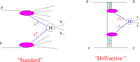
Figure 1: “Standard” vs. “Diffractive” Higgs boson production.

The potential interest of central diffractive production of the Higgs boson is illustrated in Fig.1; while standard production via gluon-gluon fusion can reach high cross-sections, the study of the Higgs boson will be uneasy due to accompanying particles and backgrounds, especially if it takes place in the low-mass range where $\gamma\gamma$ is the main observational decay mode. The original guiding line for central diffractive production $\!{}^{{\bf?}}$ is to compensate the weak cross-sections by a cleaner signal, and precise production kinematics $\!{}^{{\bf?}}$ thanks to the tagging of the diffracted protons. The basic diagrams corresponding to diffractive Higgs boson production correspond to all combinations of double gluon exchanges in various ways $\!{}^{{\bf?}}$. Their main property, which remains valid even if the gluon propagators are assumed non-perturbative, is the resummation property pictured in Fig.2; the sum of diagram contributions boils down to the on-shell convolution of (non-perturbative) gluon exchange contribution times the simplest (non-perturbative) $gg\to H$ fusion diagram contribution.

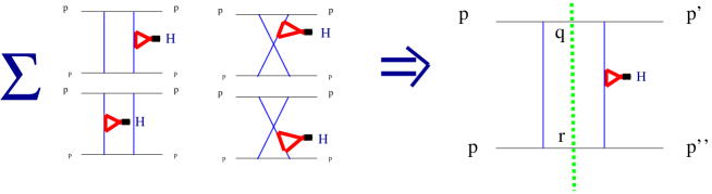
Figure 2: Higgs boson production: Factorization of lowest-order diagrams.

2 Wishes and realities

The original dynamics were presented in the framework of the simplest lowest-order diagrams. They have been considered in the framework of non-perturbative gluon propagators with a fixed $\cal O$(1) coupling constant.

What are the problems we are facing when considering “higher order” contributions? They are responsible for the production of “extra” particles which may accompany the Higgs boson production. It is not clear whether these extra particles are taken into account by the calculation of the original paper $\!{}^{{\bf?}}$. They may change drastically the estimate of Higgs production if one insists on putting a veto on the production of these extra particles. In the case extra particles are produced in the central region of rapidity, one speaks of “inclusive” diffractive production of the Higgs boson, while the term “exclusive” has been kept for the case where a strict veto on extra particles has been imposed. They are both sketched in Fig.3.

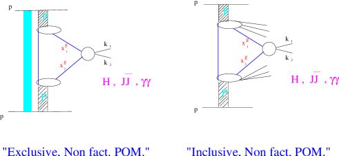
Figure 3: High mass states production: exclusive vs. inclusive. Left: The “Pomeron-induced” exclusive interaction is corrected for initial state radiation. Right: The “Pomeron-induced” inclusive interaction produces soft particles together with the heavy mass state: Higgs boson, dijet, diphoton.

On the left of Fig.3 is shown the “Pomeron-induced” model, which comes from a modification of the Bialas-Landshoff model. For exclusive production $\!{}^{{\bf?}}$ the original combination of diagrams is modified by taking into account the veto on particle radiation due to the initial states or “rapidity gap survival”. On the right, one sees a typical “inclusive” production contribution as originally proposed in Ref. $\!{}^{{\bf?}}$. In this model, the extra particles can be considered as “Pomeron remnants” in a Pomeron-Pomeron collision.

As for the models, the Pomeron-induced models inspired by the original Bialas-Landshoff approach make use of the soft Pomeron interaction to describe the diffractive coupling to the incident particles. Two other competitive approaches make a different ansatz. In the “proton-induced” model discussed in Ref. $\!{}^{{\bf?}}$, the gluon exchange + fusion mechanism is considered for purely exclusive processes, and is expected to allow for a perturbative treatment. Besides the “rapidity gap survival” (RGS) soft correction factor, the cross-section gets corrected by the perturbative Sudakov form factors. Their effect is severely cutting the production of high mass states. On the other hand, the energy dependence, being driven by the perturbative QCD rise of the gluon distribution in the proton, is quite rapid. In a third approach, the Soft Color Interaction (SCI) model $\!{}^{{\bf?}}$, the colored $gg$ fusion contribution is corrected by assuming a long distance neutralization of color.

The problem of exclusive production is that, up to know, it belongs to physicists’ wishes but not yet belongs to physics realities. Indeed, the idea of testing central diffractive production in the perspective of the Higgs boson production is to look for known color singlet massive states such as dijets or diphoton of large masses, as sketched in Fig.3. Inclusive production of massive dijets has been tested (hard diffractive production of jets has already been observed by the UA8 Collaboration at CERN and at HERA) at the Tevatron Run I $\!{}^{{\bf?}}$, and already copiously produced till the beginning of Run II. In the same time, there is yet no evidence (and thus only upper bounds) for exclusive production $\!{}^{{\bf?}}$. Hence models for exclusive production cannot “calibrate” their cross-sections on real events. Even if models of Refs. $\!{}^{{\bf?}}$ and $\!{}^{{\bf?}}$ give similar cross-section predictions for a low mass standard Higgs boson at the LHC (of the order of a few femtobarns) they greatly differ when the mass or the energy varies. On contrary the models for inclusive production, such as Refs. $\!{}^{{\bf?}}$ and $\!{}^{{\bf?}}$, are better validated thanks to their description of the observed dijet production. It is clear that the selection of viable models will be clarified by hard diffraction studies at the Tevatron.

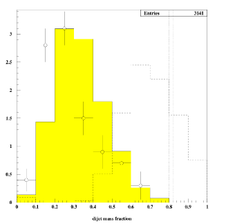
Figure 4: Dijet Mass fraction at the Tevatron. Data are from Ref.[7]; shaded histogram: model predictions from Ref.[4]; dashed (resp. dotted) contour: simulation of exclusive production at detector (resp. parton) level.

3 The “Sesame” of diffraction: understanding factorization breaking

The key question for the efficiency of hard diffractive production, in practice for the evaluation of cross-sections, is factorization breaking. It is well-known that the ratio of diffractive over non-diffractive hard events at the Tevatron compared to HERA is a factor circa 1/10 for similar kinematical variables. This factor came as a surprise, but after all, the soft interaction between the incident hadrons, absent at HERA (except for e.g. photoproduction, which is an interesting problem), is expected to interfere with the hard interaction producing the heavy state, and thus to break factorization. The whole question is to find which is the mechanism of this interference between soft and hard processes both present in the same collision. Here we only rely on phenomenological models since little is theoretically known about soft interactions, non-perturbative in terms of QCD.

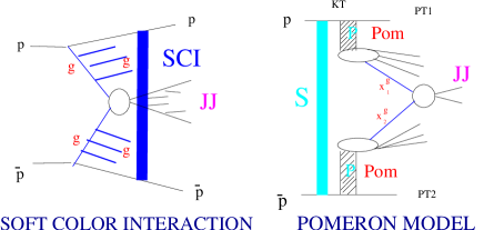
Figure 5: Models of factorization breaking. Left: “soft color interaction” ; Right: “rapidity gap survival”)

In order to illustrate the problem, we consider two popular approaches of factorization breaking mechanisms, namely the one used in the SCI approach $\!{}^{{\bf?}}$ and the RGS approaches used in (exclusive) Pomeron $\!{}^{{\bf?}}$ and proton $\!{}^{{\bf?}}$ induced models. In the former (SCI), a soft color interaction correcting the standard colored exchange may form a final singlet state allowing for diffraction. This is indeed a gap-creating mechanism. By contrast, in the RGS approaches, the initial hard, factorized, diffractive mechanism forming gaps is hidden by the interaction between initial hadrons. It is thus a gap-destroying mechanism.

Figure 6: Shape in $\Delta\Phi$ between the outgoing $p$ and $\bar{p}$ for SCI and RGS models. The upper plot is for asymmetrical cuts in $P_{T}^{2}$ ($|P_{T}^{2}(p)|>0.6$, $|P_{T}^{2}(\bar{p}p)|>0.1$ GeV²) and the lower ones for symetric cuts on $P_{T}^{2}$ ($|P_{T}^{2}(p)|>0.5$, $|P_{T}^{2}(\bar{p}p)|>0.5$ GeV²). We note the different behaviour for SCI and RGS models where the minimum is close to $\Delta\Phi\sim$ 180 degrees (resp. 130 degrees) for asymmetrical (resp.symmetric) cuts in $P_{T}^{2}$. The $\Delta\Phi$ dependence can be studied using the FPD detector, see next Fig.7.

Interestingly enough, these two models lead to very different predictions for central diffractive Higgs boson production at the LHC for a Higgs of mass around 120 GeV. While RGS models predict an overall small but sizeable cross-section of the order of the femtobarn, the SCI model predicts a completely negligible double-diffractive cross-section.

It is thus important to find ways of discrimination between models. For this sake, the experimental diffraction physics programme at the Tevatron will be crucial. As an illustration, let us consider $\!{}^{{\bf?}}$ the inclusive diffractive production of dijets and suppose that we measure the full transverse momenta of the outgoing forward proton and antiproton, namely $P_{T}$ and the azimuthal angle $\Delta\Phi$ between the two particles. It appears, see Fig.6, a significant difference between the RGS and SCI models. In Fig.6, we also compare two different RGS models, we call them model 1 $\!{}^{{\bf?}}$ and model 2 $\!{}^{{\bf?}}$, differing only through the inclusion or not of soft inelastic diffractive channels in the calculation (see $\!{}^{{\bf?}}$ for details).

The difference between RGS and SCI models can be easily traced back to the basic contrast between a gap-destroying and a gap-creating mechanism. In the former case, the correction is expressed as a destructive interference between two terms, namely

$${\cal A}(p_{T1},p_{T2},\Delta\Phi)={\cal A}^{h}-{\cal A}_{SP}\ {\bf*}{\cal A}^{h}\ \equiv\int d^{2}{\bf k}_{T}\ \left\{1-{\cal A}_{SP}\right\}({\bf k}_{T})\ {\cal A}^{h}({\bf p}_{T1}\!-\!{\bf k}_{T},{\bf p}_{T2}\!+\!{\bf k}_{T})\ ,$$

where ${\cal A}_{SP}$ is the ${\cal O}(1)$ “effective” (including inelastic diffraction, model 1) or genuine (model 2) elastic $p\bar{p}$ amplitude. ${\cal A}^{h}$ is the uncorrected hard diffractive amplitude. On the contrary, SCI models, at least in their present version (some modification of the prediction could come from a different simulation of hadronization), do not lead to striking structures since, schematically, they just weight the contributions of standard non diffractive diagrams to cross-sections by an universal probability factor. No strong interference effect is expected in this case.

An experimental measurement is not unrealistic, even if delicate, as azimuthal asymmetries could be checked at the FPD detectors included in the D0 apparatus, see Fig.7.

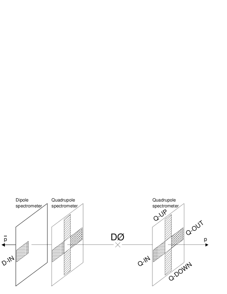
Figure 7: Schematic view of the FPD detector. This setting may allow for a study of azimuthal dependence of the outgoing hadrons.

4 Tasks in diffraction theory

At the present stage of our knowledge and since our experimentalists friends are preparing for the opening of the LHC, it is worth trying to select the valuable theoretical questions raised by the diffractive production channel of the Higgs boson.

• Evaluation of the inclusive production cross-section at the LHC. The formation of hard diffractive dijets in the central region of the Tevatron is now certain. The precise description of their observed characteristics and a motivated prediction of the energy dependence towards the LHC conditions seem possible in the next period.

• Evaluation of QCD corrections. The radiative QCD corrections are expected to be strong, under the form of Sudakov form factors in the “proton-induced” model of exclusive production. On the other hand, QCD corrections are also present in the tail of inclusive production, i.e. the end of the dijet mass spectrum, see Fig.4, of the inclusive production of dijets at Tevatron. I suggest a thorough comparison between the two approaches, and more generally on the exclusive approaches compared to the “quasi-exclusive” ones dealing with the tail of the inclusive distribution. In fact, in practice, the experimentalists will find difficult to give a criterium selecting strictly exclusive production.

• Evaluation of “soft” corrections. We have seen that there exist ways to disentangle rapidity-gap creating from rapidity-gap destroying types of models. Identifying the non-perturbative source of factorization breaking is a major task for the theoreticians interested into diffractive mechanisms. It has a major impact on the evaluation of cross-sections, since at the LHC, these effects are predicted to hide a large fraction of the interesting events (another more experimental problem, but also related with soft hadronic physics, is the piling-up due to some or many minimum-bias collisions, depending on the working luminosity).

The diffractive production could be an interesting complementary device for Higgs boson search at the LHC. Moreover, if diffractive production of known heavy states is confirmed, then it is worth investigating SUSY particle production $\!{}^{{\bf?},{\bf?}}$. It however requires some theoretical work to obtain a reasonable evaluation of the expected cross-sections. Fortunately enough, the diffractive program at the Tevatron and the search for known massive states which can be diffractively produced: dijets, diphotons, $t\bar{t}$, WW (through QED production, see e.g. $\!{}^{{\bf?}}$) will give quite a few instructive answers in the near and next-to-near future.

References

References

- [1] A. Bialas and P. V. Landshoff, Phys. Lett. B 256, 540 (1991).
- [2] G. Albrow and A. Rostovtsev, arXiv:hep-ph/0009336.
- [3] M. Boonekamp, R. Peschanski and C. Royon, Nucl. Phys. B 669, 277 (2003) [Erratum-ibid. B 676, 493 (2004)] [arXiv:hep-ph/0301244]; Phys. Lett. B 598, 243 (2004) [arXiv:hep-ph/0406061].
- [4] M. Boonekamp, R. Peschanski and C. Royon, Phys. Rev. Lett. 87, 251806 (2001) [arXiv:hep-ph/0107113].
- [5] See these proceedings: A. D. Martin, V. A. Khoze and M. G. Ryskin, arXiv:hep-ph/0507305, and references therein.
- [6] R. Enberg, G. Ingelman, A. Kissavos and N. Timneanu, Phys. Rev. Lett. 89, 081801 (2002) [arXiv:hep-ph/0203267].
- [7] T. Affolder et al. [CDF Collaboration], Phys. Rev. Lett. 85, 4215 (2000).
- [8] See these proceedings: C. Mesropian, arXiv:hep-ph/0510193; K. Goulianos [CDF Run I and Run II Collaborations], arXiv:hep-ph/0510035.
- [9] A. Kupco, C. Royon and R. Peschanski, Phys. Lett. B 606, 139 (2005) [arXiv:hep-ph/0407222].
- [10] V. A. Khoze, A. D. Martin and M. G. Ryskin, Eur. Phys. J. C18 (2000) 167, Eur. Phys. J. C24 (2002) 581.
- [11] A. Bialas, Acta Phys. Polon. B33 (2002) 2635; A. Bialas, R. Peschanski, Phys.Lett. B575 (2003) 30.
- [12] M. Boonekamp, J. Cammin, R. Peschanski and C. Royon, arXiv:hep-ph/0504199; M. Boonekamp, J. Cammin, S. Lavignac, R. Peschanski and C. Royon, arXiv:hep-ph/0506275.