Effects of Environment Dependence of Neutrino Mass versus Solar and Reactor Neutrino Data

Abstract

In this work we study the phenomenological consequences of the environment dependence of neutrino mass on solar and reactor neutrino phenomenology. We concentrate on mass varying neutrino scenarios in which the enviroment dependence is induced by Yukawa interactions of a light neutral scalar particle which couples to neutrinos and matter. Under the assumption of one mass scale dominance, we perform a global analysis of solar and KamLAND neutrino data which depends on 4 parameters: the two standard oscillation parameters, $\Delta m^{2}_{0,21}$ and $\tan^{2}\theta_{12}$, and two new coefficients which parameterize the environment dependence of the neutrino mass. We find that, generically, the inclusion of the environment dependent terms does not lead to a very statistically significant improvement on the description of the data in the most favoured MSW LMA (or LMA-I) region. It does, however, substantially improve the fit in the high-$\Delta m^{2}$ LMA (or LMA-II) region which can be allowed at 98.9% CL. Conversely, the analysis allow us to place stringent constraints on the size of the environment dependence terms which can be translated on a bound on the product of the effective neutrino-scalar ($\lambda^{\nu}$) and matter-scalar ($\lambda^{N}$) Yukawa couplings, as a function of the scalar field mass ($m_{S}$) in these models, $|\lambda^{\nu}\,\lambda^{N}|\,\left(\frac{10^{-7}\,\text{eV}}{m_{S}}\right)^{2}\leq 3.0\times 10^{-28}$ (at 90% CL) .

I Introduction

The possibility of environment dependence (ED) of the effective neutrino mass was first proposed as a possible solution to the solar neutrino deficit by Wolfenstein wolfenstein . In the Standard Model, the vector part of the standard charged current and neutral current neutrino-matter interactions contribute to the neutrino evolution equation as an energy independent potential term. The potential is proportional to the electron density and it has different sign for neutrinos and anti-neutrinos, even in the CP conserving case. It gives rise to the well-known Mikheyev-Smirnov-Wolfenstein (MSW) effect wolfenstein ; ms which is crucial in the interpretation of the solar neutrino data.

In most neutrino mass models, new sources of ED of the effective neutrino mass arise as a natural feature due to the presence of non-standard neutrino interactions with matter review . If the new interaction can be cast as a neutral or charged vector current, it will also contribute as an energy independent potential to the neutrino evolution equation. The phenomenological implications of such non-standard interactions in neutrino oscillations have been widely considered in the literature nsi ; nsi2 ; nsi3 .

New physics in the form of Yukawa interactions of neutrinos and matter with a neutral light scalar particle modify the kinetic part of the neutrino evolution equation. Such neutral scalar interactions induce a dependence of the neutrino mass on the environment Sawyer which is energy independent and has the same sign for neutrinos and anti-neutrinos. Recently, this form of ED of the neutrino mass has received renewed attention after Ref. dark1 discussed the possibility that such mass varying neutrinos (MaVaNs) can behave as a negative pressure fluid which contributes to the origin of the cosmic acceleration. This scenario establishes a connection between neutrino mass and dark energy with interesting cosmological consequences dark1 ; Peccei ; Pas .

In the MaVaNs scheme presented in Ref. dark1 , the neutrino mass arises from the interaction with a scalar field, the acceleron, whose effective potential changes as a function of the neutrino density. As a consequence, the neutrino mass depends on the neutrino density in the medium. A subsequent work, Ref. dark2 , investigated the possibility that neutrino masses depend on the visible matter density as well. Such a dependence would be induced by non-renormalizable operators which would couple the acceleron to the visible matter. This form of ED of the neutrino mass could also lead to interesting phenomenological consequences for neutrino oscillations dark2 ; Zurek ; Barger ; mymavas .

For solar neutrinos, in Ref. mymavas it was shown that, generically, due to the dependence of the neutrino mass on the neutrino density, these scenarios establish a connection between the effective $\Delta m^{2}$ in the Sun and the absolute neutrino mass scale. Due to this effect, the description of solar neutrino data worsens for neutrinos with degenerate masses. On the other hand, for hierarchical neutrino masses the dominant effect is the dependence of the neutrino mass on the visible matter density. In Ref. Barger it was shown that for some particular values of the scalar-matter couplings this effect can improve the agreement with solar neutrino data.

In this article we investigate the characteristic effects of the dependence of the neutrino mass on the matter density for solar neutrinos and reactor antineutrinos. We perform a combined analysis of solar chlorine ; sagegno ; gallex ; sk ; sno ; sno05 and KamLAND data kamland in these scenarios. Our results show that: $(i)$ the inclusion of the ED terms can lead to certain improvement of the quality of the fit in the most favour LMA-I region for well determined values of the new parameters, (in agreement with the result of Ref. Barger ), but this improvement does not hold much statistical significance; $(ii)$ the inclusion of these effects, can substantially improve the quality of the fit in the high-$\Delta m^{2}$ (LMA-II) region which can be allowed at 98.9% CL; $(iii)$ generically, the combined analysis of solar and KamLAND data results into a constraint on the possible dependence of the neutrino mass on the ordinary matter density.

In Sec. II, we introduce the general theoretical framework which we will consider in this paper. In Sec. III, we discuss how the ED modifies neutrino oscillations in matter. In Sec. IV, we examine how these modifications can affect the current allowed solar neutrino oscillation parameter region and establish the constraints that solar and reactor neutrino data can impose on the couplings to the scalar field. Finally, in Sec. V, we discuss our results and summarize our conclusions.

II Formalism

For the sake of concreteness, we consider here an effective low energy model containing the Standard Model particles plus a light scalar ($\phi$) of mass $m_{S}$ which couples very weakly both to neutrinos ($\nu_{i}$) and the matter fields $f=e,n,p$.

The Lagrangian takes the form

$${\cal L}=\sum_{i}\bar{\nu}_{i}\left(i/\!\!\!\partial\,\,-m^{0}_{i}\right)\nu_{i}+\sum_{f}\bar{f}\left(i/\!\!\!\partial\,\,-m^{0}_{f}\right)f+\frac{1}{2}\left[\phi\left(\partial^{2}-m_{S}^{2}\right)\phi\right]+\sum_{ij}\lambda^{\nu}_{ij}\bar{\nu}_{i}\nu_{j}\phi+\sum_{f}\lambda^{f}\bar{f}f\phi\;,$$ (1)

where $m^{0}_{i}$ are the vacuum mass that the neutrinos would have in the presence of the cosmic neutrino background. $\lambda^{\nu}_{ij}$ and $\lambda^{f}$ are, respectively, the effective neutrino-scalar and matter-scalar couplings. We have written a Lagrangian for Dirac neutrinos but equivalently it could be written for Majorana neutrinos.

In a medium with some additional neutrino background (either relativistic or non-relativistic) as well as non-relativistic matter (electrons, protons and neutrons), neutrinos acquire masses which obey the following set of integral equations

$$m_{ij}(r) = m^{0}_{i}\delta_{ij}-M_{ij}(r),$$

$$M_{ij}(r) = \frac{\lambda^{\nu}_{ij}}{m_{S}^{2}}\left(\sum_{f}\lambda^{f}n_{f}(r)+\sum_{a}{\lambda^{\nu}}_{aa}\int\frac{d^{3}k}{(2\pi)^{3}}\frac{M_{aa}}{\sqrt{k^{2}+M_{aa}^{2}}}f_{a}(r,k)\,\right).$$ (2)

$n_{f}(r)$ is the number density for the fermion $f$, and $f_{a}(r,k)$ is the sum of neutrino and antineutrino “$a$” occupation numbers for momentum $k$ in addition to the cosmic background neutrinos.

In the context of the dark energy-related MaVaNs models of Ref dark1 ; dark2 the scalar $\phi$ would be the acceleron – with mass in the range $m_{S}\sim 10^{-6}$–$10^{-8}$ eV – which, when acquiring a non-vanishing expectation value, $\langle\phi\rangle$, gives a contribution to the neutrino mass. This in turn implies that the acceleron effective potential receives a contribution which changes as a function of the neutrino density, so that

$$\lambda^{\nu}=\left.\frac{\partial m_{\nu}}{\partial\phi}\right|_{\langle\phi\rangle}\;.$$ (3)

$\lambda^{f}$, the effective low energy couplings of the acceleron to visible matter, come from non-renormalizable operators which couple the acceleron to the visible matter, such as might arise from quantum gravity. They can be parametrized as

$$\lambda^{f}=\tilde{\lambda}^{f}\left(\frac{m_{f}}{M_{Pl}}\right),$$ (4)

where $M_{Pl}$ is the Plank scale. Tests of the gravitational inverse square law require $\lambda^{n},\lambda^{p}\lesssim 10^{-21}$  Adelberger for any scalar with $m_{S}\gtrsim 10^{-11}$ eV.

The results in Eq.(2) and Eq.(3) correspond to the first order term in the Taylor expansion around the present epoch background value of $\phi$. In general, for the required flat potentials in these models, one needs to go beyond first order and the neutrino mass is not linearly proportional to the number density of the particles in the background. The exact dependence on the background densities is function of the specific form assumed for the scalar potential. This is mostly relevant for the neutrino density contribution to the neutrino mass.

It has been recently argued zaldarriaga that, generically, these models contain a catastrophic instability which occurs when neutrinos become non-relativistic. As a consequence the acceleron coupled neutrinos must be extremely light. Thus, in what follows we assume the vacuum neutrino masses to be hierarchical

$$0=m^{0}_{1}<m^{0}_{2}<m^{0}_{3}\;.$$ (5)

For solar neutrinos of hierarchical masses, as discussed in Ref.mymavas ; Barger , the dominant contribution to the neutrino mass is due to the matter background density. Correspondingly, we neglect the contribution to the neutrino mass from the background neutrino density and we concentrate on the matter density dependence:

$$M_{ij}(r)=\frac{\lambda^{\nu}_{ij}}{m_{S}^{2}}\sum_{f}\lambda^{f}n_{f}(r)\;.$$ (6)

This is very similar to the scenario considered in Ref.Barger .

Finally, let’s mention that by assuming Eq.(1) we do not consider the possibility of additional light mixed sterile neutrinos which may appear in some specific realizations of MaVaNs scenarios Fardon:2005wc and which can lead to other interesting effects in oscillation neutrino phenomenology and cosmology Fardon:2005wc ; Barger:2005mh ; Weiner:2005ac .

III Effects in Solar Neutrino Oscillations

The minimum joint description of atmospheric atm , K2K k2k , solar chlorine ; sagegno ; gallex ; sk ; sno ; sno05 and reactor kamland ; chooz data requires that all the three known neutrinos take part in the oscillations. The mixing parameters are encoded in the $3\times 3$ lepton mixing matrix which can be conveniently parametrized in the standard form

$$U=\begin{pmatrix}1&0&0\cr 0&{c_{23}}&{s_{23}}\cr 0&-{s_{23}}&{c_{23}}\cr\end{pmatrix}\begin{pmatrix}{c_{13}}&0&{s_{13}}e^{i{\delta}}\cr 0&1&0\cr-{s_{13}}e^{-i{\delta}}&0&{c_{13}}\cr\end{pmatrix}\begin{pmatrix}c_{21}&{s_{12}}&0\cr-{s_{12}}&{c_{12}}&0\cr 0&0&1\cr\end{pmatrix}$$ (7)

where $c_{ij}\equiv\cos\theta_{ij}$ and $s_{ij}\equiv\sin\theta_{ij}$.

According to the current data, the neutrino mass squared differences can be chosen so that

$$\Delta m^{2}_{\odot}=\Delta m^{2}_{21}\ll|\Delta m_{31}^{2}|\simeq|\Delta m_{32}^{2}|=\Delta m^{2}_{\rm atm}.$$ (8)

As a consequence of the fact that $\Delta m^{2}_{21}/|\Delta m^{2}_{31}|\approx 0.03$, for solar and KamLAND neutrinos, the oscillations with the atmospheric oscillation length are completely averaged and the interpretation of these data in the neutrino oscillation framework depends mostly on $\Delta m^{2}_{21}$, $\theta_{12}$ and $\theta_{13}$, while atmospheric and K2K neutrinos oscillations are controlled by $\Delta m^{2}_{31}$, $\theta_{23}$ and $\theta_{13}$. Furthermore, the negative results from the CHOOZ reactor experiment chooz imply that the mixing angle connecting the solar and atmospheric oscillation channels, $\theta_{13}$, is severely constrained ($\sin^{2}\theta_{13}\leq 0.041$ at 3$\sigma$ haga ). Altogether, it is found that the 3-$\nu$ oscillations effectively factorize into 2-$\nu$ oscillations of the two different subsystems: solar and atmospheric.

With the inclusion of the ED terms (Eq. (6)) it is not warranted that such factorization holds. We will assume that this is still the case and study their effect on solar and KamLAND oscillations under the hypothesis of one mass-scale dominance. Under this assumption, we parametrize the evolution equation as Barger :

$$i\frac{d}{dr}\left(\begin{array}[]{c}\nu_{e}\\ \nu_{\mu}\end{array}\right)=\left[\frac{1}{2E_{\nu}}\mathbf{U}_{\theta_{12}}\left(\begin{array}[]{cc}M_{1}^{2}(r)&M_{3}^{2}(r)\\ M_{3}^{2}(r)&(m^{0}_{2}-M_{2}(r))^{2}\end{array}\right)\mathbf{U}_{\theta_{12}}^{\dagger}+\left(\begin{array}[]{cc}V_{\rm CC}(r)&~{}0\\ 0&~{}0\end{array}\right)\right]\left(\begin{array}[]{c}\nu_{e}\\ \nu_{\mu}\end{array}\right),$$ (9)

where we have assumed the neutrinos to follow the hierarchy given in Eq.(5). Here $V_{\rm CC}(r)=\sqrt{2}G_{F}n_{e}(r)$ is the MSW potential proportional to the electron number density $n_{e}(r)$ in the medium. $\mathbf{U}_{\theta_{12}}$ is the $2\times 2$ mixing matrix in vacuum parameterized by the angle $\theta_{12}$, and $M_{i}(r)$ are the ED contributions to the neutrino masses.

In general, for given matter density profiles, Eq. (9) has to be solved numerically. As discussed in Ref.Barger in most of the parameter space allowed by KamLAND and solar data, for all practical purposes, the transition is adiabatic and the evolution equation can be solved analytically to give the survival probability

$$P_{ee}=\frac{1}{2}+\frac{1}{2}\cos 2\theta^{m}_{0,12}\cos 2\theta_{12}\,,$$ (10)

where $\theta^{m}_{0,12}$ is the effective neutrino mixing angle at the neutrino production point $r_{0}$ in the medium, explicitly given by

$$\cos 2\theta^{m}_{0,12}=\frac{(\Delta\tilde{M}_{21}^{2}(r_{0})\cos 2\tilde{\theta}_{0,12}-2E_{\nu}V_{\rm CC}(r_{0}))}{\sqrt{(\Delta\tilde{M}_{21}^{2}(r_{0})\cos 2\tilde{\theta}_{0,12}-2E_{\nu}V_{\rm CC}(r_{0}))^{2}+(\Delta\tilde{M}_{21}^{2}(r_{0})\sin 2\tilde{\theta}_{0,12})^{2}}},$$ (11)

with

$$\Delta\tilde{M}_{21}^{2}(r_{0})=2\sqrt{M_{3}^{4}(r_{0})+\left(\frac{\Delta M^{2}_{21}(r_{0})}{2}\right)^{2}}$$ (12)

$$\cos 2\tilde{\theta}_{0,12}=\frac{\displaystyle\frac{\Delta M_{21}^{2}(r_{0})}{2}\cos 2\theta_{21}-M_{3}^{2}(r_{0})\sin 2\theta_{12}}{\sqrt{M_{3}^{4}(r_{0})+\left(\displaystyle\frac{\Delta M^{2}_{21}(r_{0})}{2}\right)^{2}}}$$ (13)

and where

$$\Delta M^{2}_{21}(r_{0})=(m_{2}^{0}-M_{2}(r_{0}))^{2}-M_{1}^{2}(r_{0}).$$ (14)

As discussed in the previous section, in general, $M_{i}(r)$ can be an arbitrary function of the background matter density. For the sake of concreteness we will assume a dependence in accordance with the results obtained in the linear approximation given in Eq.(6). Furthermore, using Eq.(4), $\lambda^{e}\ll\lambda^{n}=\lambda^{p}\equiv\lambda^{N}$, so we will parametrize these terms as:

$$M_{i}(r)=\alpha_{i}\,\left[\frac{\rho(r)}{\rm(gr/cm^{3})}\right]~{}~{},$$ (15)

where $\rho$ is the matter density, and from Eq.(6) we find the characteristic value of the $\alpha$ coefficients to be

$$\alpha\sim 4.8\times 10^{23}\,\lambda^{\nu}\,\lambda^{N}\,\left(\frac{10^{-7}\text{eV}}{m_{S}}\right)^{2}\,{\rm eV}\;.$$ (16)

One must notice, however, that, as long as the transition is adiabatic, the survival probability only depends on the value of $M_{i}(r)$ at the neutrino production point. Therefore it only depends on the exact functional form of $M_{i}(r)$ via the averaging over the neutrino production point distributions.

The survival probability for anti-neutrinos, $P_{\bar{e}\bar{e}}$, which is relevant for KamLAND, takes the form

$$P_{\bar{e}\bar{e}}=1-\sin^{2}2\tilde{\theta}^{m}_{0,12}\sin^{2}\left(\frac{\Delta m^{2}_{KL}L}{2E_{\nu}}\right)\,,$$ (17)

where $\cos 2\tilde{\theta}^{m}_{0,12}$ is defined as in Eq. (11) and $\Delta m^{2}_{KL}$ is the denominator of this equation but replacing $V_{\rm CC}$ by $-V_{\rm CC}$ and assuming a constant matter density $\rho\sim 3$ gr/cm³, typical of the Earth’s crust.

To illustrate the effects of the $\alpha$ coefficients, we show in Fig. 1 the evolution of the mass eigenvalues $m_{1}$ and $m_{2}$ in matter as a function of $V_{\rm CC}E_{\nu}$ for different values of $\alpha_{2}$ (keeping $\alpha_{1}=\alpha_{3}=0$). As a reference, we also show in this figure the standard MSW evolution curve (solid line) for the oscillation parameters at $\Delta m^{2}_{0,21}=(m_{2}^{0})^{2}=8\times 10^{-5}$ eV² and $\tan^{2}\theta_{12}=0.4$, a point which explains very well both solar and KamLAND data. From this plot we can appreciate that in the region relevant to solar neutrino experiments the evolution of the mass eigenvalues is not significantly different from the MSW one if $|\alpha_{2}|\raise 1.29167pt\hbox{$\;<$\kern-7.5pt\raise-4.73611pt\hbox{$\sim\;$}}$ 10^-5 eV. For larger values of $\alpha_{2}$, such as $|\alpha_{2}|=$ 10^-4 eV, we expect solar neutrinos to be affected. On the other hand, KamLAND data is very little affected by the ED terms in this range of $\alpha_{2}$.

Figure 1 also illustrates a curious feature of these scenarios: the fact that it is possible to find a value of the matter dependence term which exactly cancels $\Delta m^{2}_{0,21}$. It can be seen, directly from Eqs. (9), that if for a particular point, $r_{0}$, in the medium, $m_{2}^{0}=M_{2}(r_{0})$ and $M_{1}=M_{3}=0$ ($\alpha_{1}=\alpha_{3}=0$) the lower mass eigenstate will be zero while the higher one will be at the corresponding value of $2V_{\rm CC}(r_{0})E_{\nu}$.

Non-adiabatic effects in the Sun can also occur. In the region of relatively small $\alpha$ parameters, non-adiabaticity occurs when the parameters are “tunned” to give a vanishing effective $\Delta m^{2}_{21}$ (the denominator of Eq. (11)). This can be achieved, for example, with $\alpha_{1}=\alpha_{2}=0$ by solving the following set of equations inside the Sun:

$$(m^{0}_{2})^{2}\cos 2\theta-2M^{2}_{3}(r)\sin 2\theta = 2E_{\nu}V_{\rm CC}(r),$$ (18)

$$(m^{0}_{2})^{2}\sin 2\theta+2M^{2}_{3}(r)\cos 2\theta = 0.$$ (19)

It can be shown that for $\alpha_{3}=i\,5.5\times 10^{-5}$ eV, $\tan^{2}\theta=0.3$ and $E_{\nu}=10$ MeV this set of equations are fulfilled at $r/R_{\odot}\sim 0.027$, and the neutrinos would suffer a non-adiabatic transition on their way out of the Sun. However, in general for the small values of the $\alpha$ parameters discussed here, these non-adiabatic effects do not lead to a better description of the solar neutrino data.

More generically, non-adiabatic effects occur for sufficiently large values of the $\alpha$ parameters so that one can disregard the standard MSW potential $V_{\rm CC}$ and the vacuum mass $m_{2}^{0}$ with respect to the matter density mass dependent terms. In this case, as seen from Eq. (11), the mixing angle inside the Sun is constant and controlled by the $\alpha^{\prime}s$. At the border of the Sun, as the density goes to zero, the mixing angle is driven to its vacuum value in a strongly non-adiabatic transition. This scenario would be equivalent to a vacuum-like oscillation for solar neutrinos with the ED of neutrino mass having to play a leading role in the interpretation of terrestrial neutrino experiments. We will leave the detailed analysis of the consequences of this type of non-adiabatic transitions for a future work.

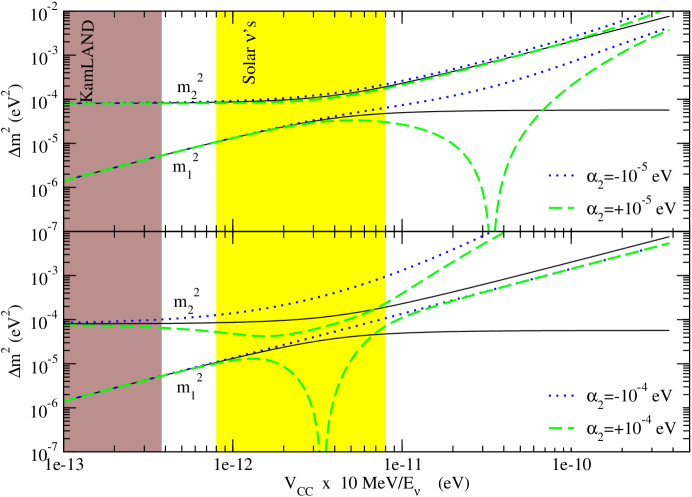
Figure 1: Evolution of the neutrino mass eigenvalues in matter. The solid lines represent the familiar MSW evolution. In this plot we have fixed $(m_{2}^{0})^{2}=8\times 10^{-5}$ eV², $\tan^{2}\theta_{12}=0.4$ and $\alpha_{1}=\alpha_{3}=0$. In the upper (lower) panel the dotted line represents the case $\alpha_{2}=-10^{-5}$ eV ($\alpha_{2}=-10^{-4}$ eV) and the dashed line the case $\alpha_{2}=+10^{-5}$ eV ($\alpha_{2}=+10^{-4}$) eV. The shaded regions correspond to typical values of $V_{\rm CC}$ in neutrino production region in the center of the Sun for the Solar $\nu$’s region, and a constant Earth crust density of 3 g/cm³, with a proton density fraction of $Y=0.5$ and neutrino energies varying from 3 to 10 MeV for the KamLAND region.

IV Constraints from Solar and Reactor Neutrino Data

We present in this section the results of the global analysis of solar and KamLAND for the specific realization discussed in the previous section. Furthermore, for simplicity, we will restrict ourselves to the case $M_{1}(r)=m_{1}=0$.

Details of our solar neutrino analysis have been described in previous papers oursolar ; pedrosolar . We use the solar fluxes from Bahcall and Serenelli (2005) BS05 . The solar neutrino data includes a total of 119 data points: the Gallium sagegno ; gallex and Chlorine chlorine (1 data point) radiochemical rates, the Super-Kamiokande sk zenith spectrum (44 bins), and SNO data reported for phase 1 and phase 2. The SNO data used consists of the total day-night spectrum measured in the pure D₂O (SNO-I) phase (34 data points) sno , plus the full data set corresponding to the Salt Phase (SNO-II) sno05 . This last one includes the NC and ES event rates during the day and during the night (4 data points), and the CC day-night spectral data (34 data points). The analysis of the full data set of SNO-II is new to this work. It is done by a $\chi^{2}$ analysis using the experimental systematic and statistical uncertainties and their correlations presented in sno05 , together with the theoretical uncertainties. In combining with the SNO-I data, only the theoretical uncertainties are assumed to be correlated between the two phases. The experimental systematics errors are considered to be uncorrelated between both phases.

For KamLAND, we directly adapt the $\chi^{2}$ map as given by the KamLAND collaboration for their unbinned rate+shape analysis kamhomepage which uses 258 observed neutrino candidate events and gives, for the standard oscillation analysis, a $\chi^{2}_{\rm min}$=701.35. The corresponding Baker-Cousins $\chi^{2}$ for the 13 energy bin analysis is $\chi^{2}_{\rm min}=13.1/11$ dof. The effect of MaVaN’s parameters in KamLAND result was calculated assuming a constant Earth density of 3 g/cm³, and assuming that KamLAND are sensitive to the vacuum value of $\Delta m^{2}_{0,21}$ and $\theta_{12}$ through an effective mass and mixing in a constant Earth density, respectivelly given by the denominator of Eq. (11) and Eq. (13), as described in Eq. (17).

In presence of the ED contribution to the masses, the analysis of solar and KamLAND data depends on four parameters: the two standard oscillation parameters $\Delta m^{2}_{0,21}=(m^{0}_{2})^{2}$, and $\tan^{2}\theta_{12}$, and the two ED coefficients, $\alpha_{2}$, and $\alpha_{3}$. In this case, in order to cover the full CP conserving parameter space we allow the $\alpha$ parameters to vary in the range

$$-\infty\leq\alpha_{2}\leq\infty\;\;\;\;\;\;\;\;\;\;\;-\infty\leq\alpha^{2}_{3}\leq\infty$$ (20)

We find the best fit point

$$\tan^{2}\theta_{12}=0.49~{} ~{}\Delta m^{2}_{0,21}=8.4\times 10^{-5}~{}{\rm eV}^{2}$$

$$\alpha_{2}=10^{-4}~{}{\rm eV}~{} ~{}\alpha_{3}=i\,2.0\times 10^{-5}~{}{\rm eV}~{}.$$ (21)

This is to be compared with the best fit point for no ED of the neutrino mass, i.e., $\alpha_{2}=\alpha_{3}=0$

$$\tan^{2}\theta_{12}=0.44~{} ~{}\Delta m^{2}_{0,21}=7.9\times 10^{-5}~{}{\rm eV}^{2}~{}.$$

$$\Delta\chi^{2}=2.5$$ (22)

where $\Delta\chi^{2}$ is given with respect to the minimum at the best fit point in Eq.(21). Thus we find that although the inclusion of the ED terms can lead to a small improvement of the quality of the fit (in agreement with the result of Ref. Barger ), this improvement is not statistically very significant leading only to a decrease of $\Delta\chi^{2}=2.5$ even at the cost of introducing two new parameters.

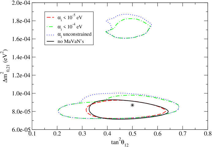
Figure 2: Allowed regions from the global analysis of solar plus KamLAND data in the $(\Delta m^{2}_{0,21},\tan^{2}\theta_{12})$ parameter space at 3$\sigma$ CL (2dof). The best fit point at $\tan^{2}\theta_{12}=0.5$ and $\Delta m^{2}_{0,21}=8.7\times 10^{-5}~{}{\text{eV}}^{2}$ is represented by the star. The standard MSW allowed region is also shown for reference.

We show in Fig. 2 the result of the global analysis of solar data plus KamLAND data in the form of the allowed two-dimensional regions at 3$\sigma$ CL in the $(\Delta m^{2}_{21,0},\tan^{2}\theta_{12})$ plane after marginalization over $\alpha_{2}$ and $\alpha_{3}$. The standard MSW allowed region is also showed for reference. As seen in the figure, allowing for ED of the neutrino masses enlarges only slightly the allowed range of $\Delta m^{2}_{21,0}$ and $\tan^{2}\theta_{12}$ in the LMA-I region. In contrast to the standard MSW analysis, where the limits on the mixing angle come basically from solar neutrinos, here it is KamLAND data that control the lower limits for the mixing angle.

Most interestingly, we also find that the description of the solar data in the high-$\Delta m^{2}$ (LMA-II) region can be significantly improved so there is a new allowed solution at the 98.9% CL. The best fit point in this region is obtained for

$$\tan^{2}\theta_{12}=0.5~{} ~{}\Delta m^{2}_{0,21}=1.75\times 10^{-4}~{}{\rm eV}^{2}$$

$$\alpha_{2}=1.3\times 10^{-4}~{}{\rm eV}~{} ~{}\alpha_{3}=i\,2.0\times 10^{-5}~{}{\rm eV}\;$$

$$\Delta\chi^{2}=8.9$$ (23)

While this region is excluded at more than 4$\sigma$ for standard MSW oscillations, it is allowed at 98.9% CL (2.55$\sigma$) in the presence of environmental effects with $|\alpha_{3}|\leq 3.2\times 10^{-5}$ and $2.8\times 10^{-5}\leq\alpha_{2}\leq 2.0\times 10^{-4}$. Basically the CL at which this region is presently allowed is determined by KamLAND data kamland because the fit to the solar data cannot discriminate between the LMA-I and LMA-II regions once the ED terms are included. Clearly this implies that this solution will be further tested by a more precise determination of the antineutrino spectrum in KamLAND.

We show in Fig.3 the survival probability for this best fit point in the high-$\Delta m^{2}$ (LMA-II) region in the presence of ED effects together with the extracted average survival probabilities for the low energy ($pp$) , intermediate energy (⁷Be, $pep$ and CNO) and high energy solar neutrinos (⁸B and $hep$) from Ref. Barger . For comparison we also show the survival probability for conventional oscillations ($\alpha_{i}=0$) with the same values of $\Delta m^{2}_{21,0}$ and $\theta_{12}$. From the figure it is clear that the inclusion of the ED parameters, leads to an improvement on the description of the solar data for all the energies being this more significant for intermediate- and high-energy neutrinos.

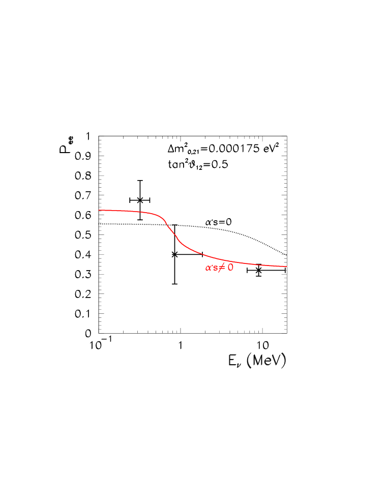
Figure 3: $\nu_{e}$ survival probability in the Sun versus neutrino energy for the best fit point in the high-$\Delta m^{2}$ region in the presence of ED effects (Eq. (23)). The dotted line is the survival probability for conventional oscillations ($\alpha_{i}=0$) with the same values of $\Delta m^{2}_{21,0}$ and $\theta_{12}$. These survival probabilities have been obtained for neutrinos produced around $x=0.05$ as it is characteristic of ⁸B and ⁷Be neutrinos. The data points are the extracted average survival probabilities for the low energy ($pp$) , intermediate energy (⁷Be, $pep$ and CNO) and high energy solar neutrinos (⁸B and $hep$) from Ref. Barger .

On the contrary, unlike for the case of non-standard neutrino interactions discussed in Ref.nsi2 ; nsi3 , the low-$\Delta m^{2}$ (LMA-0) region is still disfavoured at more than 3 sigma by the global KamLAND and solar data analysis even in the presence of the new “kinetic-like” ED effects discussed here. This is due to the different energy dependence of the new physics effects in the two cases. For the “kinetic-like” effects it is not possible to suppress matter effects in the Earth for the high energy neutrinos (to fit the SK and SNO negative results on the day-night asymmetry within LMA-0) without spoiling the agreement of the survival probability at intermediate energies with the result of the radiochemical experiments.

Conversely, the global analysis of solar and KamLAND data results into the constraint of the possible size of the ED contribution to the neutrino mass. This is illustrated in Fig.4 where we show the result of the global analysis in the form of the allowed two-dimensional regions in the $(\alpha_{2},\alpha_{3})$ parameter space after marginalization over $\Delta m^{2}_{0,21},\tan^{2}\theta_{12}$. The full regions correspond to 1$\sigma$, 95% and 3 $\sigma$ CL while the curves correspond to 90 and 99% CL. As seen in the figure, for CL $>$ 1.1$\sigma$ the regions are connected to the $\alpha_{2}=\alpha_{3}=0$ case and they are always bounded. In other words, the analysis show no evidence of any ED contribution to the neutrino mass and there is an upper bound on the absolute values of the corresponding coefficients.

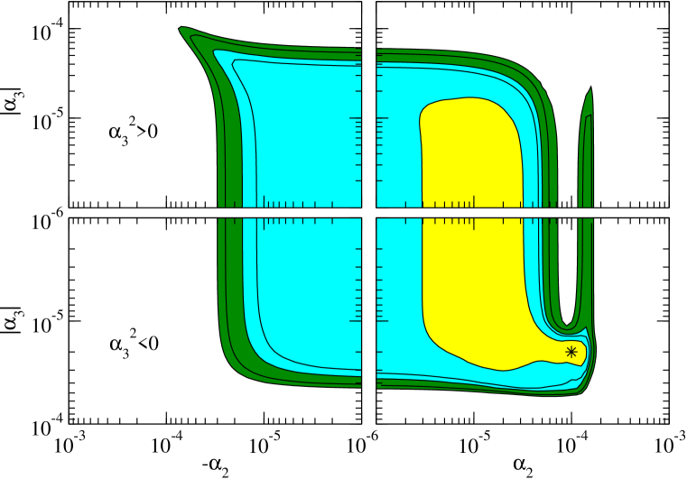
Figure 4: Allowed regions from the global analysis of solar and solar plus KamLAND data in the $(\alpha_{2},\alpha_{3})$ parameter space. The curves correspond to 1$\sigma$, 90%, 95%, 99% and 3$\sigma$ CL (2dof). The best fit point at $\alpha_{2}=10^{-4}~{}{\text{eV}}$ and $\alpha_{3}=i\,2.0\times 10^{-5}~{}{\text{eV}}$, represented by a star, is also shown.

Our previous discussion at the end of Sec. III on the behavior of the mass eigenvalues shown in Fig. 1 when $M_{2}\rightarrow m_{2}^{0}$, is the reason behind the exclusion of the narrow gulf around $\alpha_{2}\approx 10^{-4}$ eV. In this region, unless $\alpha_{3}$ is negative and not too small, it is not possible to explain solar neutrino data.

In order to quantify the bound on MaVaN’s parameters, we display in Fig.5 the dependence of the global $\chi^{2}$ on $\alpha_{2}$ ($\alpha_{3}$) after marginalization over $\Delta m^{2}_{0,21}$, $\tan^{2}\theta_{12}$ and $\alpha_{3}$ ($\alpha_{2}$).

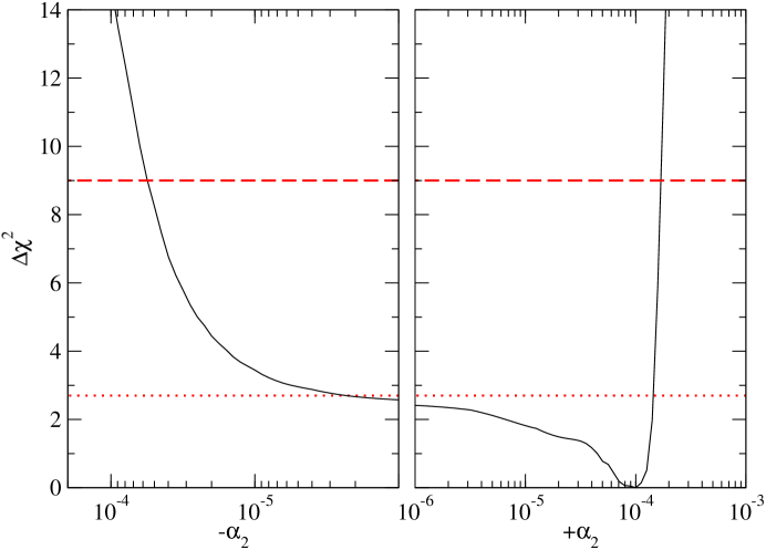
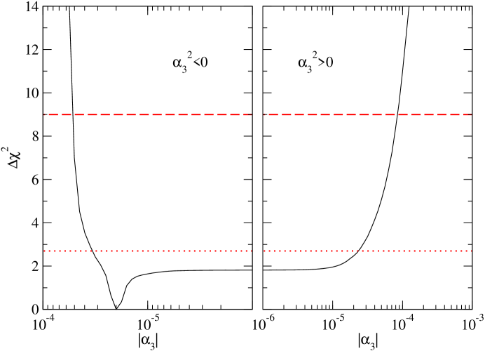
Figure 5: Dependence of $\chi^{2}$ on the ED parameters $\alpha_{2}$ (upper panel) and $\alpha_{3}$ (lower panel) after marginalization over the other three parameters.

From the figure we read the following 90% CL (3 $\sigma$), bounds (with 1dof)

$$-2.2\times 10^{-5}\leq\alpha_{2}/{\rm eV}\leq 1.4\times 10^{-4} (-5.6\times 10^{-5}\leq\alpha_{2}/{\rm eV}\leq 1.7\times 10^{-4})$$ (24)

$$|\alpha_{3}|/{\rm eV}\leq 2.3\times 10^{-5} (|\alpha_{3}|/{\rm eV}\leq 8.4\times 10^{-5})\;\;{\rm for}\;\;\alpha_{3}^{2}>0$$ (25)

$$|\alpha_{3}|/{\rm eV}\leq 3.4\times 10^{-5} (|\alpha_{3}|/{\rm eV}\leq 5.2\times 10^{-5})\;\;{\rm for}\;\;\alpha_{3}^{2}<0$$ (26)

These bounds can be converted into a limit on the product of the characteristic effective neutrino-scalar and matter-scalar couplings. For example, at 90% CL,

$$|\lambda^{\nu}\,\lambda^{N}|\,\left(\frac{10^{-7}\,\text{eV}}{m_{S}}\right)^{2}\leq 3.0\times 10^{-28}\,.$$ (27)

We can compare this bound with those derived from tests of the gravitational inverse square law (ISL) which require the coupling of the scalar to nucleons $|\lambda^{N}|\lesssim 10^{-21}$  Adelberger for any scalar with $m_{S}\gtrsim 10^{-11}$ eV. Thus we find that if the scalar also couples to neutrinos with coupling

$$\lambda^{\nu}\gtrsim 3.0\times 10^{-7}\left(\frac{m_{S}}{10^{-7}\,\text{eV}}\right)^{2}$$ (28)

the analysis of solar and KamLAND data yields a more restrictive constraint on the matter-scalar couplings than ISL tests.

Finally, we want to comment on the possible model-dependence of these results. There are two main sources of arbitrariness in our derivations: the choice of $m_{1}=M_{1}(r)=0$ and the assumption that the $M_{i}$ are linearly dependent on the matter density. Indeed their effect is the same: departing of any of these assumptions results into a different functional dependence of the effective neutrino masses with the point along the neutrino trajectory, $m_{i}(r)$.

As discussed in the previous section, the basic assumption behind our results is that neutrino evolution in matter is adiabatic. As long as this is the case, the survival probability only depends on the value of the effective neutrino masses at the neutrino production point and the final results depend very mildly on the exact functional form of $m_{i}(r)$. As a consequence the generic results will still be valid: there will be a slight improvement on the quality of the fit in the LMA-I region, there will be a substantial improvement of the quality of the fit on the LMA-II region and generically the combined analysis of solar and KamLAND data will result into a bound on the strength of the new contributions. Of course, the exact numerical values of the corresponding ED couplings will be different. But the order of magnitude of the bound on the product of the Yukawa couplings in Eq. (27) will hold.

V Discussion

We have investigated the phenomenological consequences of a scalar induced ED of the effective neutrino mass in the interpretation of solar and reactor neutrino data. For the sake of concreteness, we consider an effective low energy model containing the Standard Model particles plus a light neutral scalar ($\phi$) of mass $m_{S}$ which couples very weakly both to neutrinos ($\nu_{i}$) and the matter fields $f=e,n,p$. This is described in Sec. II and its consequences to neutrino oscillations in the Sun is discussed in Sec. III.

Assuming the neutrino masses to follow the hierarchy $0=m^{0}_{1}<m^{0}_{2}<m^{0}_{3}$, we have performed a combined analysis of the solar neutrino data (118 data points) and KamLAND (17 data points) in the context of this effective model. Our analysis, which is described in Sec. IV, depends on 4 parameters: the two standard oscillation parameters $\Delta m^{2}_{0,21}=(m^{0}_{2})^{2}$, and $\tan^{2}\theta_{12}$, and the two ED coefficients, $\alpha_{2}$, and $\alpha_{3}$. We found the best fit point at: $\tan^{2}\theta_{12}=0.49$, $\Delta m^{2}_{0,21}=8.4\times 10^{-5}~{}{\rm eV}^{2}$, $\alpha_{2}=10^{-4}~{}{\rm eV}$ and $\alpha_{3}=i\,2.0\times 10^{-5}~{}{\rm eV}$. This point corresponds to a decrease of $\Delta\chi^{2}_{\text{min}}=-2.5$ in comparison to the minimum in the case where no ED is considered. We conclude that in spite of the inclusion the two extra parameters, the improvement of the quality of the fit in the most favoured LMA-I MSW region is not very statistically significant.

Most interestingly, we find that the description of the solar data in the high-$\Delta m^{2}$ (LMA-II) region can be significantly improved and there is a new allowed solution at the 98.9% CL. The best fit point in this region is obtained for $\tan^{2}\theta_{12}=0.5$, $\Delta m^{2}_{0,21}=1.75\times 10^{-4}~{}{\rm eV}^{2}$, $\alpha_{2}=1.3\times 10^{-4}~{}{\rm eV}$ and $\alpha_{3}=i\,2.0\times 10^{-5}~{}{\rm eV}$. This solution will be further tested by a more precise determination of the antineutrino spectrum in KamLAND.

In any case, our data analysis permit us to considerably limit the size of the $\alpha$ coefficients (see Eq. (26)) and from that to derive a limit on the product of the effective neutrino-scalar and matter-scalar Yukawa couplings depending on the mass of the scalar field (Eq. (27)). In particular, for neutrino-scalar couplings $\lambda^{\nu}\gtrsim 3.0\times 10^{-7}(m_{S}/10^{-7}\text{eV})^{2}$ our analysis of solar and KamLAND data yields a more restrictive constraint on the matter-scalar couplings than gravitational ISL tests.

These scenarios will be further tested by the precise determination of the energy dependence of the survival probability of solar neutrinos, in particular for low energies lowe .