Chern-Simons and winding number in a tachyonic electroweak transition

Abstract:

We investigate the development of winding number and Chern-Simons number in a tachyonic transition in the SU(2) Higgs model, motivated by the scenario of cold electroweak baryogenesis. We find that localized configurations with approximately half-integer winding number, dubbed half-knots, play an important role in this process. When the Chern-Simons number adjusts locally to the winding number, the half-knots can stabilize and acquire half-integer Chern-Simons number as well. We present two examples from numerical simulations: one half-knot that stabilizes early and one that gives rise to a late sphaleron transition. We also study the winding number distribution after the transition and present new results on the development of the Chern-Simons susceptibility.

1 Introduction

Baryogenesis, the creation of the baryon asymmetry in the universe, is a long standing problem in cosmology. It dates back to 1967, when Sakharov suggested that the baryon asymmetry is not an initial condition of the universe, but might be created later in a process based on particle physics [1]. This idea has gained support from the inflationary scenario, since inflation is supposed to have diluted any pre-existing asymmetry. Sakharov formulated his well-known conditions for baryogenesis: baryon number conservation, C, and CP must be violated, and a state of non-equilibrium must prevail.

Of the many particle physics scenarios that have been proposed in the past decades implementing such a process, electroweak baryogenesis [2, 3, 4] is interesting in that it suggested the possibility to explain the baryon asymmetry using mostly Standard Model physics. In this scenario the baryon number violation is caused by the anomaly that relates a change in baryon number $B$ to a change in Chern-Simons number $N_{\rm CS}$ of the electroweak gauge fields:

$$\Delta B=3\langle\Delta N_{\rm CS}\rangle.$$ (1)

Furthermore the Standard Model violates C, it has a CP violating phase in the CKM quark mixing matrix, and the out-of-equilibrium conditions can be provided by an electroweak phase transition. This phase transition was supposed to be caused by the lowering temperature of the universe, and to be sufficiently out of equilibrium it had to be of first order. However subsequent work has shown that for the experimentally allowed range of the Higgs mass, the electroweak phase transition is only a crossover (see e.g. [5]). It is widely believed that a crossover transition is too close to equilibrium for creation of the asymmetry. Furthermore, the CKM CP violation has been found to be much too small [6, 7, 8].

A few years ago, new scenarios were proposed [9, 10], in which electroweak baryogenesis takes place during a tachyonic transition. In such a transition the effective mass term in the Higgs potential starts being positive, and can change sign due to the coupling to an inflaton field, as in hybrid inflation [11]. The accompanying instability can lead to strongly out-of-equilibrium conditions with large occupation numbers in the Higgs and gauge fields, during which the energy in the Higgs field is transferred to the other fields by wave-like ‘rescattering’. The process is called tachyonic preheating [12]. During the transition there can be substantial changes in the Chern-Simons number, and also the baryon number via the anomaly equation (1). The universe was assumed to be cold after electroweak-scale inflation, so initially the transition takes place at practically zero temperature.

In subsequent papers the scenario was further refined and tested. Considerations of quantum corrections led to a change of model to inverted hybrid inflation [13], in which the inflaton rolls away from the origin instead of towards it. In [14] it was shown how WMAP data constrain the parameters of a model and it was noted that it might be falsified by the LHC. The transition was studied by analytic and numerical methods [15, 16, 17, 18, 19], and the magnitude of the asymmetry generated by a form of CP violation was computed in [16, 19].

The CP violating term in the Lagrangian that was used in [19] does not occur in the Standard Model. Of course, one is also interested in the CP violation from the CKM matrix. As mentioned above, this CP violation has been estimated to be much too small for baryogenesis [6, 7, 8], but these estimates do not seem to apply to a tachyonic transition at zero temperature. In fact, it has been suggested [20] that the effect might be much larger in this case. It is therefore important to make sure whether the CP violation of the Standard Model is sufficient to produce the baryon asymmetry.

Trying to investigate this problem by numerical simulation with three generations of fermions is a practically impossible task. Instead we have in mind a more tractable approach: if the changes of $N_{\rm CS}$ occur in a certain type of local field configuration, we could estimate the produced asymmetry by simulating only this local configuration. There is reason to believe that the change of $N_{\rm CS}$ indeed occurs in local configurations: in [18] evidence is found for local structures in numerical simulations, and in [10, 13] it is suggested that topological defects called textures play a role in this process. The presence of a texture depends on the winding number of the Higgs field $N_{\rm w}$. In the vacuum $N_{\rm CS}=N_{\rm w}$. A texture is a configuration which has winding number different from the Chern-Simons number. It is unstable and can decay either by changing the winding number or the Chern-Simons number. In [21, 22] a scenario for electroweak baryogenesis is investigated in which the change of Chern-Simons number occurs during the decays of textures. The textures were supposed to be formed directly after a first order electroweak phase transition, and the produced asymmetry was estimated by simulating a single texture and its decays. Such an approach was investigated further in ref. [23], where it was concluded that it is unlikely to be successful and that the asymmetry depends on too many variables to bypass a fully-fledged numerical simulation. We believe this conclusion is not so clear cut and consider it worthwhile to understand more fully the mechanism that changes Chern-Simons numbers in tachyonic transitions.

In this paper we study the production of winding and Chern-Simons number in a tachyonic transition. We shall argue that instead of textures, related configurations with half-integer winding number are important. We call such configurations half-knots. These typically occur in regions where the Higgs magnitude has a small minimum. They can be stabilized when the Chern-Simons number density adjusts to the winding number density and the Higgs field relaxes towards its ground state, leaving a blob-like half-knot both in winding number and in Chern-Simons number. Half-knots have a rather high winding number density in their center and can be visualized in numerical simulations. We present some examples in detail.

In section 2 we review the Chern-Simons number, winding number and winding configurations in this model. Next we turn to the tachyonic transition and discuss our expectations with respect to the half-knots in this transition, in section 3. In section 4 we present the results of the numerical simulations, and we discuss the results in section 5.

2 Winding in the SU(2) Higgs model

In this section we review some topological features of the SU(2) Higgs model, since it is the part of the Standard Model that plays a dominant role in the tachyonic transition. First we introduce the model and define the Higgs winding number and the Chern-Simons number. Then we discuss topological defects that may play a role in the transition: textures, sphalerons and half-knots.

2.1 SU(2) Higgs model

The action is given by

$$S=-\int d^{4}\!x\left[\frac{1}{2g^{2}}\mbox{Tr}F_{\mu\nu}F^{\mu\nu}+\frac{1}{2}\,\mbox{Tr}\left[\left(D_{\mu}\Phi\right)^{\dagger}D^{\mu}\Phi\right]+\lambda\left(\frac{1}{2}\,\mbox{Tr}\left[\Phi^{\dagger}\Phi\right]-\frac{v^{2}}{2}\right)^{2}\right],$$ (2)

where the field strength is $F_{\mu\nu}=\partial_{\mu}A_{\nu}-\partial_{\nu}A_{\mu}-i[A_{\mu},A_{\nu}]$, the vector potential can be written as $A_{\mu}=A_{\mu}^{a}\tau^{a}/2$, and the covariant derivative acting on the Higgs field is $D_{\mu}\Phi=(\partial_{\mu}-iA_{\mu})\Phi$. We use a metric with signature (-1,1,1,1) and for the Higgs field we use the matrix notation:

$$\Phi=\begin{pmatrix}\varphi_{d}^{*}&\varphi_{u}\\ -\varphi_{u}^{*}&\varphi_{d}\end{pmatrix}=\frac{\rho}{\sqrt{2}}\;\Omega,\quad\rho^{2}=2(\varphi_{u}^{*}\varphi_{u}+\varphi_{d}^{*}\varphi_{d}),\quad\Omega(x)\in\mbox{SU(2)}.$$ (3)

We call $\rho$ the Higgs length. The Higgs and W masses are given by $m_{\rm H}=\sqrt{2\lambda}\;v$ and $m_{W}=gv/2$, we also use the notation

$$\mu=\sqrt{\lambda v^{2}}.$$ (4)

As part of an extended theory, the mass term $-\lambda v^{2}\frac{1}{2}\,\mbox{Tr}\,\Phi^{\dagger}\Phi$ is to be replaced by an effective mass term

$$\mu_{\rm eff}^{2}\frac{1}{2}\,\mbox{Tr}\,\Phi^{\dagger}\Phi,$$ (5)

where $\mu_{\rm eff}^{2}$ depends on time through the coupling to another field (inflaton). Initially it is positive, and when it changes to negative the tachyonic transition starts. Eventually $\mu_{\rm eff}^{2}$ will relax to the Standard Model value

$$\mu_{\rm eff}^{2}\to-\lambda v^{2}=-\mu^{2}.$$ (6)

The rate of change of $\mu_{\rm eff}$ depends on further details of the theory.

Throughout this paper we we use the so-called ‘temporal gauge’ $A_{0}=0$, which still leaves the freedom to do time-independent gauge transformations.

2.2 Topology in the SU(2) Higgs model

The non-conservation of baryon number in the Standard Model follows from the anomaly in the divergence of the baryon current,

$$\partial_{\mu}j^{\mu}_{B} = 3\,q,$$ (7)

$$q = \frac{1}{32\pi^{2}}\,\epsilon^{\kappa\lambda\mu\nu}\mbox{Tr}\,F_{\kappa\lambda}F_{\mu\nu}=\partial_{\mu}j^{\mu}_{\rm CS}.$$ (8)

Here 3 is the number of generations and $j^{\mu}_{\rm CS}$ is the Chern-Simons current; $q$ is sometimes called the topological charge density, since, for classical fields, and in euclidean space-time, its integral over a four-dimensional manifold without boundary is an integer, the topological charge. Taking the expectation value of (7) in the initial (Heisenberg) state and integrating between (real) times 0 and $t$ gives

$$B(t)-B(0)=\int_{0}^{t}dx^{0}\int d^{3}x\,\langle 3q\rangle=3\langle N_{\rm CS}(t)-N_{\rm CS}(0)\rangle,$$ (9)

with $B=\langle\int d^{3}x\,J^{0}_{B}\rangle$ the baryon number and

$$N_{\rm CS}=\int d^{3}x\,j^{0}_{\rm CS},\quad j^{0}_{\rm CS}=-\frac{1}{16\pi^{2}}\epsilon^{jkl}\mbox{Tr}\left[A_{j}\left(F_{kl}+i\frac{2}{3}A_{k}A_{l}\right)\right],$$ (10)

the Chern-Simons number operator. We assumed that $\int d^{3}x\,\partial_{k}\langle j^{k}_{\rm CS}\rangle$ vanishes, e.g. in a model with periodic boundary conditions, or because the fields vanish sufficiently fast at spatial infinity.

At this stage the Chern-Simons number and current are still operators, whereas the baryon number $B$ is a c-number in the way we have written it. In the following we shall make a classical approximation (see section 3), and therefore we assume from now on that all fields are classical. Note that $N_{\rm CS}(t)$ and $N_{\rm CS}(t)-N_{\rm CS}(0)$ are generically not integers.

The winding number of the Higgs field is given by

$$N_{\rm w} =\int d^{3}x\,n_{\rm w},$$ (11)

$$n_{\rm w} =\frac{1}{24\pi^{2}}\,\epsilon^{ijk}\mbox{Tr}\left[\partial_{i}\Omega\Omega^{-1}\partial_{j}\Omega\Omega^{-1}\partial_{k}\Omega\Omega^{-1}\right],$$ (12)

where $\Omega$ is given implicitly by (3); this is a valid definition as long as $\rho\neq 0$ everywhere. Classical vacuum configurations are given by

$$\Phi=\frac{v}{\sqrt{2}}\,\Omega,\hskip 28.45274ptA_{j}=-i\partial_{j}\Omega\Omega^{-1},\hskip 28.45274pt\Omega\in\mbox{SU(2)}.$$ (13)

Here $\Omega$ is arbitrary. It is easy to check that in the vacuum (13) the winding number density $n_{\rm w}$ equals the Chern-Simons number density $j^{0}_{\rm CS}$.

The winding number (11) and Chern-Simons number (10) are not gauge-invariant; they change by an integer under so-called large gauge transformations. As a consequence a vacuum configuration can have any integer winding number and Chern-Simons number, as long as they are equal $N_{\rm CS}=N_{\rm w}$. Under gauge transformations $N_{\rm CS}$ and $N_{\rm w}$ change by the same amount, so that the difference $N_{\rm w}-N_{\rm CS}$ is gauge-invariant. The change in time of $N_{\rm CS}$ as defined by the integral over $q$ in (9) is also gauge invariant.

In the following we briefly discuss two well-known configurations that can play a role in changing the Chern-Simons and/or the winding number, namely the sphaleron and the texture.

2.3 Sphaleron

A sphaleron transition is a change from a vacuum with winding numbers $N_{\rm CS}=N_{\rm w}=n$, to another vacuum with $N_{\rm CS}=N_{\rm w}=n\pm 1$. It has been shown [25, 26] that the system must pass an energy barrier. The static and unstable configuration at the minimum barrier height is called a sphaleron, and its energy is the sphaleron energy. This configuration has vanishing Higgs length in the center, so that the winding number is not defined: it jumps by an integer exactly at the transition. The Chern-Simons number of a sphaleron is precisely $1/2$ (up to an integer).

The sphaleron energy $E_{\rm sph}$ is proportional to $v/g$, and approximately 10 TeV. Because of this high energy-barrier, tunneling through the barrier (which corresponds to an instanton-like event) is strongly suppressed. Therefore the baryon number is effectively conserved at low temperatures. At higher temperatures the suppression is weaker because of thermal fluctuations over the barrier. It is also useful to interpret this in terms of an effective temperature-dependent Higgs length $\langle\rho\rangle<v$ and an effective barrier height $\propto\langle\rho\rangle/g$. Above the electroweak phase-transition temperature $\langle\rho\rangle$ vanishes and sphaleron transitions occur unsuppressed. During a tachyonic electroweak transition there are also frequent fluctuations over the barrier, as observed numerically in the susceptibility $\langle N_{\rm CS}^{2}(t)\rangle$ [18, 19].

2.4 Texture

Without gauge fields, a texture is a configuration with a nonzero winding number $N_{\rm w}$, with the Higgs length equal to the vacuum value everywhere, and with only gradient energy. According to Derrick’s theorem [27] such a configuration is unstable because its energy can be lowered indefinitely by shrinking it. Numerical simulations show that textures shrink quickly, and it was argued in [24] that in the end the configuration looses its winding number and decays into outgoing waves.

For the SU(2) Higgs model a natural extension of a texture is a gauged texture: a configuration with Chern-Simons number different from the winding number: $N_{\rm CS}-N_{\rm w}=\pm 1$. One can think of an initial configuration in which the gauge fields are pure-gauge with integer Chern-Simons number and Higgs length equal to the vacuum value. Just as in the global case, a gauged texture is unstable. There are basically two ways in which it can decay [21, 22]: when its size is smaller than approximately $1/m_{W}$, it decays by changing the winding number, and when it is larger it decays by changing the Chern-Simons number. In either case $N_{\rm CS}-N_{\rm w}\to 0$ and the configuration can spread indefinitely into outgoing waves.

2.5 Half-knot

Although the total winding number in a finite volume with periodic boundary conditions is integer, in practice there is no reason to find local configurations with nearly integer winding number or Chern-Simons number. This is because there is no mechanism that would create such configurations, as there is, for example, energy minimization for monopoles. Consequently the winding number density can be spread out over the volume. However as we will argue below, there will be high winding number density regions where the Higgs length is very small. The total winding number in such a region is typically not integer, but close to $1/2$, which is why we call these configurations half-knots.

One dimension

We illustrate this idea first in the simpler but analogous one dimensional case with a complex scalar field $\Phi$ and global symmetry group U(1),

$$\Phi=\frac{1}{\sqrt{2}}\,(\phi_{1}+i\phi_{2})=\frac{\rho}{\sqrt{2}}\;\Omega,\quad\Omega\in U(1).$$ (14)

The winding number density is ($x\equiv x^{1}$)

$$n_{\rm w}=-\frac{i}{2\pi}\,\Omega^{*}\partial_{x}\Omega=\frac{1}{2\pi\rho^{2}}\,(\phi_{1}\partial_{x}\phi_{2}-\phi_{2}\partial_{x}\phi_{1}).$$ (15)

In a coordinate patch were we can write $\Omega(x)=\exp[i\omega(x)+\mbox{const.}]$ we also have $n_{\rm w}=\frac{1}{2\pi}\,\partial_{x}\omega$.

In order to gain some intuition, let us consider the following simple form

$$\phi_{1}(x)=\cos(x)-.95,\hskip 28.45274pt\phi_{2}(x)=\sin(x),$$ (16)

for which the Higgs length $\rho$ has a minimum when $x$ is close to zero. This configuration is shown in a parametric plot in figure 1. In this plot the Higgs length $\rho$ is the distance from the origin, and the change of phase corresponds to the ’winding’ of the curve around the origin. When there is a small Higgs length, the phase changes quickly (in this case approximately by an amount $+\pi$) and there is a high winding number density. We can see this also in figure 2, where the Higgs length squared $\rho^{2}$ and the winding number density are plotted. We call such a region with small Higgs length and large winding number density a half-knot. Note that the total winding number is integer (in this case $+1$), but that only part of the winding number density is concentrated in a small region. The rest of is distributed approximately homogeneously over the rest of space.

We can formalize the half-knot by approximating $\phi_{1}$ and $\phi_{2}$ locally (around $x=0$) by a linear form

$$\phi_{\alpha}=c_{\alpha}+d_{\alpha}x,\quad\alpha=1,2.$$ (17)

This corresponds to approximating the circle near the origin by a straight line, and gives

$$n_{\rm w} = \frac{1}{2\pi\rho^{2}}\,(c_{1}d_{2}-c_{2}d_{1}),$$ (18)

$$\rho^{2} = c_{\alpha}c_{\alpha}+2c_{\alpha}d_{\alpha}x+d_{\alpha}d_{\alpha}x^{2},$$ (19)

and a contribution to the winding number

$$N_{\rm w}^{\rm peak}\equiv\int_{-\infty}^{\infty}dx\,n_{\rm w}=\frac{1}{2}\,\mbox{sgn}(c_{1}d_{2}-c_{2}d_{1})=\pm\frac{1}{2}.$$ (20)

We have extended the integral to $\pm\infty$, but of course, the linear approximation breaks down somewhere and the integral is to be interpreted as the contribution from a peak in the winding density.

Three dimensions

In this subsection we introduce half-knots for the three dimensional case. As in the one dimensional case we parametrize the Higgs field by real fields

$$\Phi=\frac{1}{\sqrt{2}}\,\left(\phi_{4}1+i\phi_{a}\tau^{a}\right),$$ (21)

A simple example is a configuration that can locally be approximated by Fourier modes:

$$\phi_{\alpha}(x)=\sin({\bf x}\cdot{\bf k}_{\alpha}-\epsilon_{\alpha}),\quad\alpha=1,\ldots,4.$$ (22)

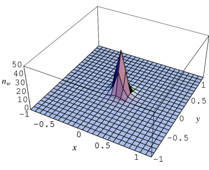
Figure 3: The Higgs length $\rho^{2}$ (left) and the winding number density $n_{\rm w}$ (right) for the configuration (22), (23), as function of $x$ and $y$, with $z=0.05$.

The Higgs length $\sqrt{\phi_{\alpha}\phi_{\alpha}}$ will be small near the origin if all the $\epsilon_{\alpha}\ll 1$. In order to get a local minimum and not a long streamline of small Higgs length, the vectors ${\bf k}_{\alpha}$ should span three dimensional space. In figure 3 we plotted the Higgs length and the winding number density as a function of $x=x^{1}$ and $y=x^{2}$, in a slice through $z=x^{3}=0.05$, for the case

$${\bf k}_{1}=(1,0,0),\;{\bf k}_{2}=(0,1,0),\;{\bf k}_{3}=(0,0,1),\;{\bf k}_{4}=(0,0,1),\quad\epsilon_{1}=\epsilon_{2}=\epsilon_{3}=0.1,\;\epsilon_{4}=0.$$ (23)

The integrated winding number in a box $x,y,z\in[-0.5,0.5]$ around the peak is found to be $0.43$, and it does not depend strongly on the integration volume.

The 3d half-knot may be formalized similar to the 1D case by using a linear approximation in a region where the Higgs length is small (on the scale of $m_{\rm H}$),

$$\phi_{\alpha}({\bf x})=c_{\alpha}+d_{\alpha k}x^{k}.$$ (24)

Then the winding number density is given by

$$n_{\rm W}=\frac{1}{12\pi^{2}\rho^{4}}\,\epsilon_{jkl}\epsilon_{\alpha\beta\gamma\delta}\partial_{j}\phi_{\alpha}\partial_{k}\phi_{\beta}\partial_{l}\phi_{\gamma}\,\phi_{\delta},$$ (25)

and in the linear approximation this gives

$$n_{\rm W}=\frac{1}{2\pi^{2}\rho^{4}}\,\det M,$$ (26)

where $M$ is the $4\times 4$ matrix consisting of the column vectors $d_{\alpha 1}$, $d_{\alpha 2}$, $d_{\alpha 3}$, $c_{\alpha}$,

$$\det M=(1/6)\epsilon_{jkl}\,\epsilon_{\alpha\beta\gamma\delta}\,d_{\alpha j}\,d_{\beta k}\,d_{\gamma l}\,c_{\delta}.$$ (27)

The integral over the winding density can be done by shifting coordinates, ${\bf x}\to{\bf x}^{\prime}$,

$$x^{k}=x^{\prime k}-g^{kl}d_{\alpha l}\,c_{\alpha},$$ (28)

where $g^{kl}$ is the inverse of $f_{kl}$ defined by

$$f_{kl}=d_{\alpha k}d_{\alpha l},\quad g^{kl}f_{lm}=\delta^{k}_{m}.$$ (29)

In terms of the shifted coordinates we have

$$\phi_{\alpha}=c^{\prime}_{\alpha}+d_{\alpha k}x^{\prime k},\quad c^{\prime}_{\alpha}=c_{\alpha}-d_{\alpha k}g^{kl}d_{\beta l}c_{\beta},\quad c^{\prime}_{\alpha}d_{\alpha k}=0,$$ (30)

and the length of the Higgs field is given by

$$\rho^{2}=c^{\prime}_{\alpha}c^{\prime}_{\alpha}+f_{kl}\,x^{\prime k}x^{\prime l}.$$ (31)

The winding number of the half-knot equals

$$\int d^{3}x\,n_{\rm W}=\frac{1}{2}\,{\rm sgn}\det M=\pm\frac{1}{2}.$$ (32)

Since $f_{kl}$ is a positive matrix, the center (maximum winding-number density) of the half-knot is at ${\bf x}^{\prime}=0$, and it has an ellipsoidal shape (surface of constant $n_{\rm w}$). Its energy density has a constant contribution from the gradients, $\frac{1}{2}\partial_{k}\phi_{\alpha}\partial_{k}\phi_{\alpha}=\frac{1}{2}d_{\alpha k}d_{\alpha k}$, whereas the contribution from $\frac{1}{4}\lambda(\rho^{2}-v^{2})^{2}$ drops off away from the center.

When $\rho$ vanishes in the center as a consequence of dynamics, so when the vector $c_{\alpha}$ vanishes, the winding number may or may not flip sign, depending on how the vector $c_{\alpha}$ recovers from zero. A pure-Higgs half-knot can decay by spreading. With a gauge field present, the Chern-Simons number may adjust to the winding number locally, such that the difference between winding and Chern-Simons number essentially vanishes.

Half-knots occur generically near the moment textures decay by changing their winding number, or near sphaleron transitions, because at these moments the Higgs length vanishes at a point. But half-knots are more general, for example, they occur in random field configurations, e.g. initial conditions for classical evolution. It is not clear yet at this stage that they are relevant, but in the simulations we will see that they are.

3 Winding in the tachyonic transition

In this section we discuss the evolution of winding number and Chern-Simons number in a fast tachyonic transition. First we will review the relevant features of such a transition. After that we will discuss the importance of half-knots and differentiate between early and late half-knots.

3.1 Tachyonic transition

At the onset of the tachyonic transition, when the effective mass parameter $\mu_{\rm eff}^{2}$ of the Higgs field changes sign, the universe is assumed to be in a homogeneous state with $\langle\Phi\rangle\approx 0$. As $\mu_{\rm eff}^{2}\to-\mu^{2}$, the Higgs potential becomes unstable near the origin and the low momentum modes of $\Phi$ grow very fast. Since the couplings in the Standard Model are fairly weak, it makes sense to study this process neglecting interactions. In this approximation the Fourier modes of the Higgs field satisfy

$$\ddot{\Phi}_{\alpha}({\bf k},t)+[\mu_{\rm eff}^{2}(t)+{\bf k}^{2}]\Phi_{\alpha}({\bf k},t)=0,$$ (33)

which can be solved exactly for the initial stage where $\mu_{\rm eff}^{2}\approx-M^{3}t$ [28, 15] (choosing $t=0$ as the onset of the transition). It turns out that the unstable field modes, i.e. the modes with ${\bf k}^{2}<-\mu_{\rm eff}^{2}$ grow very fast; the number of unstable modes also grows when $-\mu_{\rm eff}^{2}$ increases.

Interactions

An estimate for the moment that interactions set in is given by the time that the average Higgs field reaches the point where the second derivative of the potential vanishes. This is around $m_{\rm H}t=4.8$, for an instantaneous quench and $m_{\rm H}/m_{W}=\sqrt{2}$ [19]. There are both self-interactions of the Higgs field and interactions with the gauge field. The self-interactions slow down the growth of the Higgs field, and eventually lead to an oscillation near the vacuum state. The interactions with the gauge fields lead to a strong growth of the gauge fields [17, 18]. The oscillation of the Higgs field is damped by the interactions, and when more fields are added in a realistic situation, this suppression is expected to be even stronger. Eventually the energy will be distributed over all modes, and the system thermalizes.

Instantaneous quench

As in [16, 17, 19], we make in this paper the approximation that the change of the potential is instantaneous in order to obtain the most dramatic effects,

$$\mu_{\rm eff}^{2}(t) = +\mu^{2},t<0,$$ (34)

$$= -\mu^{2},t>0.$$

Moreover we do not consider the inflaton field in our simulations. In this quenching approximation the modes of the Higgs field grow exponentially fast, $\Phi_{\alpha}({\bf k},t)\propto\exp[\sqrt{\mu^{2}-{\bf k}^{2}}\,t]$ [16, 19].

Classical approximation

Another approximation that we use is the classical approximation. Intuitively one can see that the fields can be considered to be classical, because the Bose fields grow exponentially fast and the occupation numbers are therefore quickly much larger than one. For the gauge field the occupation numbers become substantial only after the Higgs current in its equation of motion has grown sufficiently large, which typically takes a few $m_{\rm H}^{-1}$ units of time [17]. The approximation is implemented as follows [16, 19]. Before the instantaneous quench the fields are in the zero-temperature ground state corresponding to positive $\mu_{\rm eff}^{2}=\mu^{2}$. Neglecting interactions this corresponds to a gaussian distribution, which can be followed until it becomes classical and a switch to classical evolution can be made. However, because quantum and classical evolution are formally the same for gaussian systems, this switch can already be made at time zero, directly after the quench. The classical evolution is computed from the fully non-linear equations of motion, including the interactions. Making the switch early on also enables a more gradual inclusion of the effect of the interactions. We draw a number of Higgs field configurations from the classical part of the gaussian distribution, and take these configurations as initial conditions for the system after the quench. For simplicity, the initial gauge potentials are set to zero, whereas the $SU(2)$ electric fields are calculated from Gauss’ law [19]. Then we evolve each of these configurations according to the classical equations of motion. In the end we compute expectation values by averaging over the initial distribution.

The classical approximation for a tachyonic transition has been compared with quantum methods like the 2PI-method in [29], and it turned out that the two approximations agreed for the times and couplings used here, giving further support for both.

3.2 Winding and Chern-Simons number densities

In the initial conditions for the tachyonic transition the gauge fields are negligible, and since the gauge potentials are zero in our implementation, the Chern-Simons number density is zero. The Higgs field initially has fluctuations around zero, and therefore it has nonzero winding number density. Since the initial conditions are random, the winding number density will be randomly distributed over the volume. The total winding number in the volume will be integer, and does not have to be zero.

When the system thermalizes and the temperature decreases, the Chern-Simons number will approach the winding number. If the winding number would not change during the process, the Chern-Simons number, approaching the initial winding number, would be determined by the initial conditions, and CP violating interactions could not influence the final outcome.

In reality the winding number does change during the process, and this makes it possible that CP violation creates an asymmetry. The winding number can change when the Higgs length becomes zero in a point, and as we argued in the previous section there will be half-knots around such points. There are two periods when the Higgs has a chance to be small and change of winding is likely to occur: early in the transition when the Higgs field starts from a small fluctuation, and later on, when the Higgs length bounces back due to its self-interaction, or just any interactions, e.g. scattering of non-linear waves.

In both periods half-knots will occur; we call them early and late half-knots respectively.

3.3 Early half-knots

In the initial conditions of the tachyonic transition, the Higgs field has small fluctuations around zero. The number density of minima of the Higgs length is, depending on the initial conditions, roughly proportional to $k_{\rm max}^{3}$ where $k_{\rm max}$ is the largest wavenumber that is initialized. Because of the peculiar feature of the tachyonic transition that modes grow faster as their wavelengths are larger, this number density of minima will quickly decrease. Hence initially there are many half-knots, but their number quickly decreases.

Some half-knots will manage to survive longer. When a half-knot still exists when the gauge fields start to become important, the Chern-Simons number density in these regions can adjust to the winding number density. When the Chern-Simons number becomes approximately equal to the winding number in a blob, the covariant derivative $D_{i}\Phi$ becomes small, the gradient energy diminishes and the half-knot becomes stable.

The early half-knots are perhaps not so important for baryogenesis. In principle CP violation could cause an imbalance in the formation and decay of the number of half-knots and anti-half-knots. However in this early period there are no interactions yet, and CP violation cannot have acted. Also when the early half-knots stabilize and survive CP violation is not important because then the winding number does not change. So we expect for possible effects of CP violation, we should look at the late half-knots.

3.4 Late half-knots

The Higgs length can also become small later in the transition. For example this can happen when the Higgs field bounces back in its potential, or because of interactions in general. In this case there will be late half-knots in which the winding can change. Because interactions are important to create these half-knots, also CP violating interactions can influence this process. There may also be longer lived half-knots, not stabilized by the gauge fields, whose probability to decay is influenced by the stronger CP violation at later times.

4 Numerical simulations

In this section we first describe briefly the setup of our simulations, and then present the results.

4.1 Setup

In [19] numerical simulations were described with the $SU(2)$ Higgs model, using the approximations described in section 3.1, and with an extra CP violating term in the action. For the present work we extended the computer code of [19] to be able to observe the winding-number density and a local quantity $n_{\rm CS}$ closely related to the Chern-Simons number density (see below). We do not use the CP violation of the code of [19] because at this point we are interested in the mechanism of winding number and Chern-Simons number production, and not yet in the creation of the asymmetry.

The simulation was performed on a $60^{3}$ lattice, with periodic boundary conditions and with a lattice spacing of 0.35 $m_{\rm H}^{-1}$, such that the physical volume was $L^{3}=(21\,m_{\rm H}^{-1})^{3}$. The initial conditions mentioned in 3.1 are the “just-a-half” initial conditions as defined in [16, 19]. Effectively this means that only the growing modes, with momentum $k$ smaller than $\mu$, are initialized with probability given by the vacuum state. Furthermore we took $\lambda/g^{2}=1/4$, which is equivalent to $m_{\rm H}/m_{W}=\sqrt{2}$. (We shall also present some results for $m_{\rm H}/m_{W}=2$.) For the determination of the initial conditions, which are set by quantum fluctuations, we also have to fix $g^{2}$. We chose $g^{2}=4/9$. See [19] for more details on the numerical implementation.

The density $n_{\rm CS}$ is defined as

$$n_{\rm CS}({\bf x},t)=\int_{0}^{t}dt^{\prime}\,q({\bf x},t^{\prime}),$$ (35)

where $q$ is the gauge-invariant topological charge density given in (8). Since $q=\partial_{\mu}j_{\rm CS}^{\mu}$ and the Chern-Simons current is zero for our initial conditions,

$$n_{\rm CS}({\bf x},t)=j^{0}_{\rm CS}({\bf x},t)+\partial_{k}\int_{0}^{t}dt^{\prime}\,j^{k}_{\rm CS}({\bf x},t^{\prime}).$$ (36)

So $n_{\rm CS}$ differs from $j^{0}_{\rm CS}$ by a divergence and they both integrate to $N_{\rm CS}$. In the following we shall call $n_{\rm CS}$ the Chern-Simons density, for simplicity, but it should be kept in mind that it is not equal to $j^{0}_{\rm CS}$.

4.2 Results

4.2.1 One typical trajectory

In order to investigate classical field configurations we look at single trajectories. In this subsection we consider one typical trajectory.

Total $N_{\rm w}$ and $N_{\rm CS}$ as function of time in typical run

The variables considered in [19] were the spatial average of the Higgs length squared

$$\overline{\rho^{2}}=L^{-3}\int d^{3}x\,\rho^{2},$$ (37)

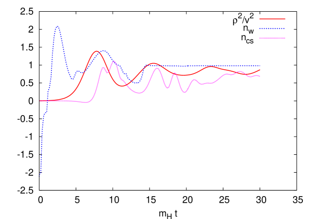
Figure 4: Results of a typical run for times $m_{\rm H}t=0$ to $m_{\rm H}t=30$. Plotted are $\overline{\rho^{2}}/v^{2}$, the total winding number $N_{\rm w}$ and total Chern-Simons number $N_{\rm CS}$.

the winding number $N_{\rm w}$ and the Chern-Simons number $N_{\rm CS}$. In figure 4 we show the evolution of these variables in time for our typical trajectory, from $m_{\rm H}t=0$ up to $m_{\rm H}t=30$. The winding number $N_{\rm w}$ fluctuates initially, and later stays put at an integer. The initial fluctuations indicate that there must be zeroes in the Higgs length. In the continuum these fluctuations would be between integers (a ‘devil’s staircase’), but here they appear as smoothed out by the lattice discretization.

We also see that the Chern-Simons number starts only when the average Higgs length is already rather large, and that at the later times $N_{\rm CS}\approx N_{\rm w}$. (Occasionally we also have seen trajectories for which the two differed at $m_{\rm H}t=30$ by a number of order 1, and only at much later times $N_{\rm CS}$ approached $N_{\rm w}$ (sometimes this took as long as $m_{\rm H}t\approx 500$).

3D pictures of $n_{\rm w}$ and $n_{\rm CS}$

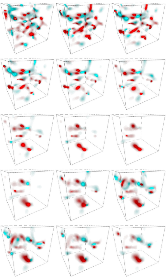
Figure 5: Winding number density $n_{\rm w}$ from $m_{\rm H}t=1$ to $m_{\rm H}t=15$. Red (dark) is positive, blue (light) is negative.

Next we look at the densities of the winding number and Chern-Simons number in this trajectory. Figure 5 displays the winding number density in the three dimensional simulation volume from times $m_{\rm H}t=1$ to $m_{\rm H}t=15$. Note that the box has periodic boundary conditions. Red (dark) indicates positive density, blue (light) negative. In the beginning there are many ’blobs’ in winding number density. We will argue below for two specific cases that these blobs are half-knots with a small Higgs length $\rho$ in their center. Sometimes they change sign. The number of blobs decreases first until approximately time $m_{\rm H}t=9$, then it increases until approximately $m_{\rm H}t=13$ after which it decreases again. Some of the early blobs that are there already from the beginning survive all the time. The blobs that appear after time $m_{\rm H}t=9$ seem to be uncorrelated to the blobs that were there before. We call these new blobs the late blobs.

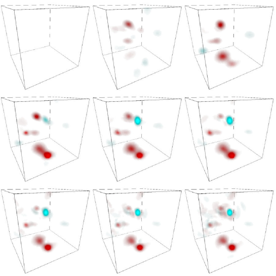
Figure 6: Chern-Simons number density $n_{\rm CS}$ from $m_{\rm H}t=7$ to $m_{\rm H}t=15$. Before $m_{\rm H}t=7$ the Chern-Simons number density is negligibly small. Red (dark) is positive, blue (light) is negative.

In figure 6 the Chern-Simons number density is shown from times $m_{\rm H}t=7$ to $m_{\rm H}t=15$. Before $m_{\rm H}t=7$ the Chern-Simons number density is negligibly small. Also in the Chern-Simons number density there are blobs. These blobs are correlated with the winding number blobs.

Small Higgs length means a lot of winding

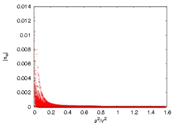
Figure 7: The absolute value of the winding number density $|n_{\rm w}|$ versus the Higgs length for all lattice points in the simulation volume, at time $m_{\rm H}t=6$.

We argued above that regions with small Higgs length have typically a large winding number density. This is confirmed in the simulations. In figure 7 the absolute value of the winding number density $|n_{\rm w}|$ is plotted versus the normalized Higgs length $(\rho/v)^{2}$ for each point on the lattice. The configuration of the typical trajectory at time $m_{\rm H}t=6$ is used, when the gauge fields are still unimportant. We see that $|n_{\rm w}|$ and $(\rho/v)^{2}$ are correlated such that, when the Higgs length on a lattice point is small, the winding number density is typically large.

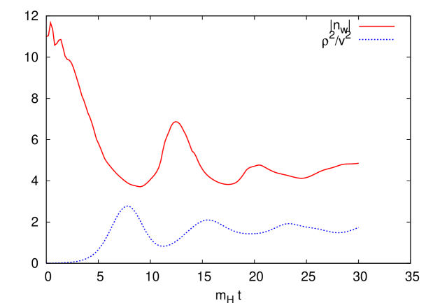
Figure 8: The integral $\int d^{3}x\,|n_{\rm w}|$ and the spatial average of the squared Higgs length versus $m_{\rm H}t$.

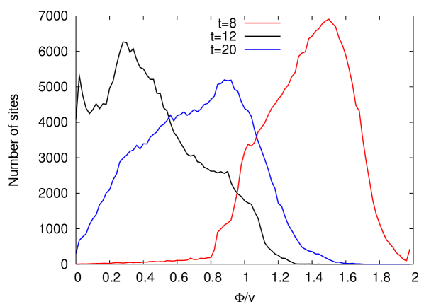
Figure 9: Histograms that display the distribution of the Higgs length on the lattice at times $m_{\rm H}t=8$, 12 and 20.

A consequence of this correlation is that when the average Higgs length is small, there will typically be more winding blobs. We saw this already in the three dimensional pictures of the winding number density: there were less winding blobs around time $m_{\rm H}t=8$, when the average Higgs length is large. We can show this more quantitatively, by plotting [30] $\int d^{3}x\,|n_{\rm w}|$ in figure 8. We see in this figure that the peak in $\int d^{3}x\,|n_{\rm w}|$ at $m_{\rm H}t\approx 20$ is much smaller than the corresponding one at $m_{\rm H}t\approx 12$. This agrees with the fact that there are much less lattice points with small Higgs length at $m_{\rm H}t=20$. We can also see this from the histograms in figure 9. We call the blobs that are created in minima of the Higgs length, second (third, …) generation blobs.

Correlation between winding number and Chern-Simons number

Because the Higgs and gauge fields interact, $n_{\rm w}$ and $n_{\rm CS}$ are correlated. This could already be seen in the three dimensional pictures, but we can also calculate the correlation

$$C({\bf r},t)=\frac{\int d^{3}x\,[n_{\rm CS}({\bf x},t)-\overline{n_{\rm CS}}(t)][n_{\rm w}({\bf x}+{\bf r},t)-\overline{n_{\rm w}}(t)]}{\sqrt{\int d^{3}x\,[n_{\rm CS}({\bf x},t)-\overline{n_{\rm CS}}(t)]^{2}}\sqrt{\int d^{3}y\,[n_{\rm w}({\bf y},t)-\overline{n_{\rm w}}(t)]^{2}}},$$ (38)

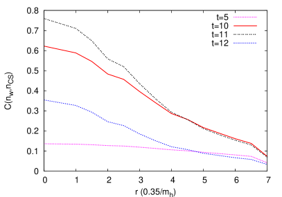
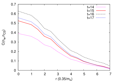
Figure 10: The correlation $C({\bf r},t)$ between $n_{\rm CS}$ and $n_{\rm w}$, defined in (38), versus $r=|{\bf r}|$ at various times.

where the ‘over-bar’ denotes the spatial average, as in (37). This correlator is plotted versus $r=|{\bf r}|$ at various times in figure 10. It shows a spatial correlation developing on distances of order $m_{\rm H}^{-1}$, modulated in time and showing a tendency to diminish at later times.

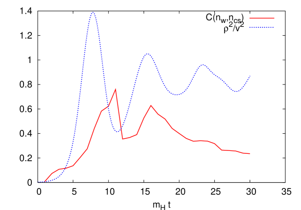
Figure 11: The correlation $C(0,t)$ versus time.

It is also instructive to plot its value at $r=0$ versus time, see figure 11. We see that the correlation $C({\bf 0},t)$ develops already at early times, it peaks at times $m_{\rm H}t\approx 12$ and 16, and there is a rapid drop after the first peak. This drop occurs when the average Higgs length has become small after its first maximum, and $\int d^{3}x\,|n_{\rm w}|$ is on the rise again (cf. figure 7). We interpret this as being caused by the creation of many new winding blobs when the Higgs length is small again, half-knots that are uncorrelated with the $n_{\rm CS}$. When $C({\bf 0},t)$ peaks for a second time the average Higgs length is large again and $\int d^{3}x\,|n_{\rm w}|$ is low. We suspect that this is because the winding blobs that still exist when the average Higgs length is large, exist already for some time and the Chern-Simons number density has had some time to adjust. Later on the correlation decreases, which is presumably caused by random fluctuations.

In the following two subsections we zoom in on two blobs, first on an early blob and then on a late survivor.

4.2.2 Early blob

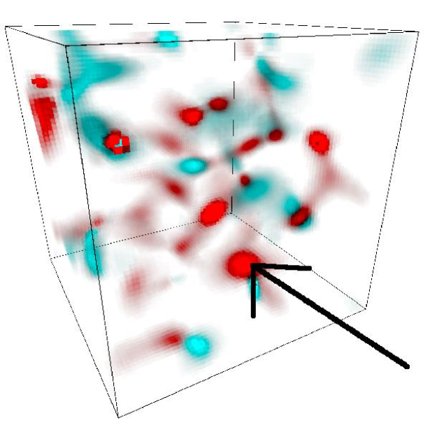
Figure 12: The winding number density at time $m_{\rm H}t=1$ of the same run as used before. The blob that we consider in this section is indicated by the arrow.

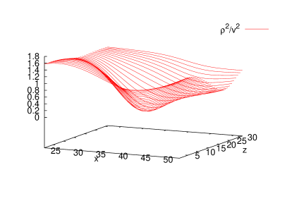
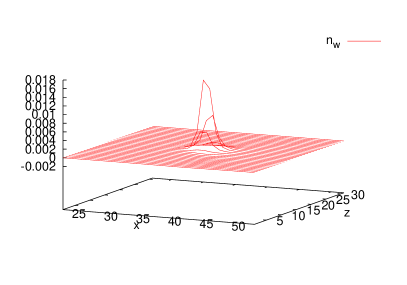
Figure 13: Left the Higgs length (vertical) at time $m_{\rm H}t=2$ is plotted at the position of the blob, as function of the $x$ and $z$ coordinates (a vertical slice). Right the winding number density at time $m_{\rm H}t=2$ is plotted for the same slice through the blob.

For the early blob we take the one indicated by the arrow in figure 12. Let us first look at the distributions of the Higgs length and the winding number density in this blob. In a vertical slice in the $xz$-directions through the center of the blob, the Higgs length and the winding number density are plotted in figure 13, at time $m_{\rm H}t=2$. The Higgs length has a minimum and the winding number has a large peak at this minimum. These figures look very similar to the analytical example in figure 3.

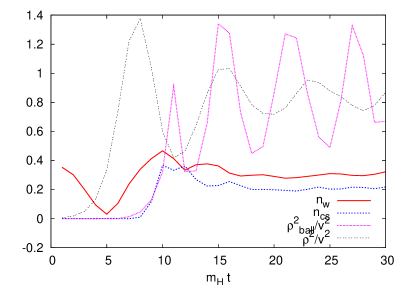
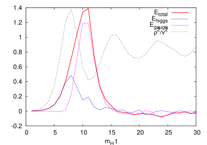
Figure 14: Left: $N_{\rm w}^{\rm ball}$, $N_{\rm CS}^{\rm ball}$ and $\overline{\rho^{2}}^{\rm ball}$, for a ball with a radius of 6 lattice units ($2.1\,m_{\rm H}^{-1}$) around the center of the blob. Right: excess energy, $[\int_{\rm ball}d^{3}x\,(\epsilon-\overline{\epsilon})]/E_{\rm sph}$, in the same ball and its contributions from the Higgs field and the gauge fields.

Next we have calculated the sums of some quantities in a ball around the center of the blob. For this we had to determine the position of the center, which is slightly ambiguous. We did it by defining the center as the point where the winding number density is maximal. The position of the center can change a bit at different times, so we determined the center at each time step. In the left panel of figure 14 we show the integrated winding number density

$$N_{\rm w}^{\rm ball}=\int_{\rm ball}d^{3}x\,n_{\rm w},$$ (39)

integrated Chern-Simons number density

$$N_{\rm CS}^{\rm ball}=\int_{\rm ball}d^{3}x\,n_{\rm CS},$$ (40)

and the volume-averaged Higgs length

$$\overline{\rho^{2}}^{\rm ball}=\int_{\rm ball}d^{3}x\,\rho^{2}\Big{/}\int_{\rm ball}d^{3}x\,1,$$ (41)

for a ball of radius 6 lattice units, corresponding to 2.1 $m_{\rm H}^{-1}$, as a function of time. For reference the Higgs length averaged over the full simulation volume is also shown.

The winding number in the ball first decreases until $m_{\rm H}t=5$, then increases until $m_{\rm H}t=10$ and afterwards stays approximately constant near a value of 0.3. The Chern-Simons number becomes visible from $m_{\rm H}t\approx 8$ onwards, has a small peak and stays constant near 0.2 after $m_{\rm H}t\approx 13$. The winding number and Chern-Simons number end up being close to each other. The average Higgs length in the ball grows only much later than the one in the full volume, and also oscillates with a somewhat higher frequency. It also exhibits much less damping, which is suggestive of oscillons [31, 32]. We will comment later on the dip in the winding number at time $m_{\rm H}t=5$.

The right panel of figure 14 shows the energy in the same ball with radius 2.1 $m_{\rm H}^{-1}$. We display the excess energy above the average energy relative to the sphaleron energy, i.e. $\int_{\rm ball}d^{3}x\,(\epsilon-\overline{\epsilon})/E_{\rm sph}$, where $\epsilon$ is the energy density and $\overline{\epsilon}$ its average over the total volume. The average energy density is simply that of the origin of the Higgs potential, $\overline{\epsilon}=m_{\rm H}^{4}/16\lambda$, and the sphaleron energy for $m_{\rm H}=\sqrt{2}\,m_{W}$ is $E_{\rm sp}\approx 3.78\,(4\pi m_{W}/g^{2})$ (see e.g. [33]), and so $\int_{\rm ball}d^{3}x\,\overline{\epsilon}/E_{\rm sp}\approx 0.29$. Hence, the sphaleron energy in this plot is at 0.71.

We show the total energy in the ball as well as its contributions from the Higgs and the gauge fields (the contribution from the covariant derivative is allocated to the Higgs fields). We see that the gauge fields contribute most to the energy. It is remarkable that the peak in the total energy occurs at a time where the average Higgs length in the ball has its first maximum, that the peak is significantly higher than the sphaleron energy, and that the energy has already fallen back to the average already shortly after $m_{\rm H}$t = 15. Evidently, a strong energy flow into and out of the ball is taking place. At the later times $N_{\rm CS}^{\rm ball}$ has roughly the same value as $N_{\rm w}^{\rm ball}$.

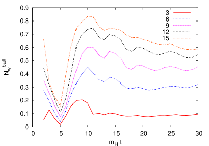
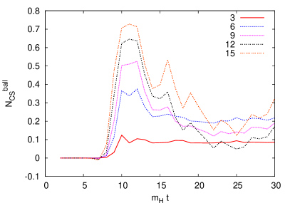
Figure 15: $N_{\rm w}^{\rm ball}$ (left) and $N_{\rm CS}^{\rm ball}$ (right) for balls with varying radii, increasing from 3 lattice distances up to 15 lattice distances.

To see how these results depend on the radius of the ball we show in figure 15 the winding number and Chern-Simons number in balls with increasing radii, from 3 up to 15 lattice units. They clearly depend on the radius, and for the larger balls $N_{\rm w}^{\rm ball}$ increases above 1/2. This may be caused by another blob of the same sign that is close (cf. figure 5, e.g. at time $m_{\rm H}t=15$ the distance between the centers of the two blobs is about 13 lattice units).

Here we return to the dip that we observed at $m_{\rm H}t=5$ in figure 14. From figure 15 we see that the dip is also there for larger radii of the ball; apparently the winding number is not flowing out of the ball, but is really decreasing. In the continuum this can only occur when the Higgs length $\rho$ is exactly zero somewhere. But on the lattice the we will miss already a significant amount of winding number when the spatial size of the winding number peak becomes smaller than a lattice unit. Hence we interpret the observed dip as a lattice artefact, signaling a half-knot in the center of which the Higgs length decreases (which makes the peak sharper) until $m_{\rm H}t=5$, and increases again after that.

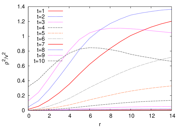
Figure 16: Profiles of the normalized Higgs length $\rho^{2}(r)/v^{2}$ for times $m_{\rm H}t=1$ to $m_{\rm H}t=10$. On the horizontal axis is the distance from the center, $r$, in lattice units (0.35 $m_{\rm H}^{-1}$).

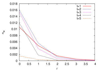
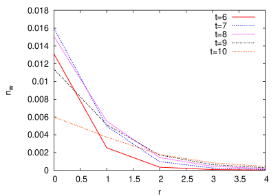
Figure 17: As in figure 16 for $n_{\rm w}(r)$ for times $m_{\rm H}t=1$ to $m_{\rm H}t=5$ (left) and until $m_{\rm H}t=10$ (right).

Further insight can be obtained from the profiles of the Higgs length and the winding-number density around the center of the blob, $\rho(r)$ and $n_{\rm w}(r)$. They are plotted in figures 16 and 17, for times $m_{\rm H}t=1$ to 10. The profiles are determined by averaging at fixed distances $r$ from the center over all directions. For the position of the center we used the same values as in figure 14.

From the Higgs length profiles we see that, while the Higgs length in the bulk grows steadily from the beginning, in the center of the blob it remains very small up to time $m_{\rm H}t\approx 6$, and starts to grow only after that. At the latest time $\rho(r)$ looks like an oscillation about the equilibrium value $\approx v$. The winding number density profile is already well defined at time $m_{\rm H}t=1$. It then shrinks and becomes steeper towards the center, $m_{\rm H}t=2$ and 3. This shrinking and steepening appears to get blurred by lattice artefacts at $m_{\rm H}t=4,5,6$ (note that the profiles here are shown on a much smaller scale than the $\rho$-profile in figure 16), and as mentioned earlier, we believe this is the reason for the dip in $N_{\rm w}^{\rm ball}$ at $m_{\rm H}t=5$. From time $m_{\rm H}t=10$ the winding number profile broadens.

We conclude that we have witnessed the formation of a half-knot, that nearly decayed by shrinking, but got ‘saved’ by the gauge field adjusting its Chern-Simons number density and diminishing the Higgs gradient density $|D_{i}\Phi|^{2}$. Remarkably, this adjustment goes together with a big jump in gauge-field energy. At later times the well-dressed blob carries no excess energy, and the process has led to a local change in the total Chern-Simons number.

4.2.3 Late transition

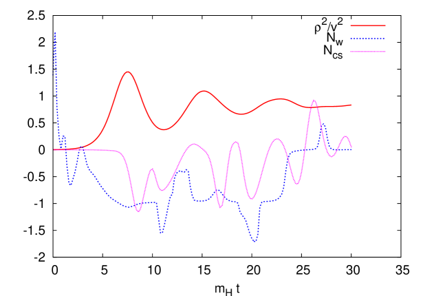
Figure 18: The analog of figure 4 for the trajectory with a late transition, $\overline{\rho^{2}}/v^{2}$, total winding number $N_{\rm w}$ and total Chern-Simons number $N_{\rm CS}$.

Above we have seen (in the three dimensional pictures 5, 6 and the $|n_{\rm w}|$ graph 8) that new blobs are created when the average Higgs length is small. Sometimes the winding number $N_{\rm w}$ changes in such a blob. Here we present an example of such a late blob in which the winding number changes. It comes from another trajectory than the one used before. Figure 18 shows the evolution of $\overline{\rho^{2}}$, $N_{\rm w}$ and $N_{\rm CS}$ in this run up to time $m_{\rm H}t=30$. Note that the winding number changes from $-1$ to 0 between $m_{\rm H}t=23$ and $m_{\rm H}t=24$. This change takes place in the blob that we are going to consider.

Figure 19 shows 3D plots of the winding and Chern-Simons number densities at times $m_{\rm H}t=23$ and 24. The change of the winding number occurs in the blob that changes sign at the top of the box. At the same position there is a positive Chern-Simons number density both before and after the change of winding number.

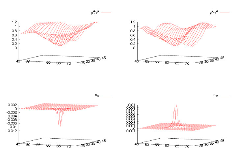
Figure 20: Upper plots: Higgs length as function of the $x$ and $z$ coordinates through the blob. Left is at time $m_{\rm H}t=23$, right at time $m_{\rm H}t=24$. Lower plots: the corresponding winding number density.

In figure 20 the Higgs length and the winding number density in a horizontal slice through the blob are shown for times $m_{\rm H}t=23$ and $m_{\rm H}t=24$. There is a pronounced minimum in the Higgs length at the place of the peak in the winding number density. The latter changes quite abruptly from negative to positive.

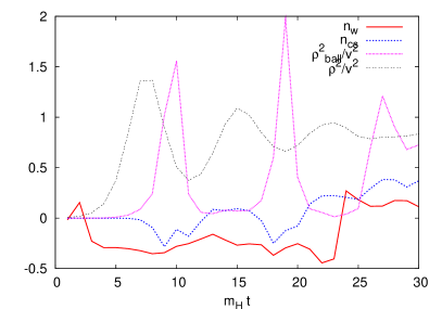
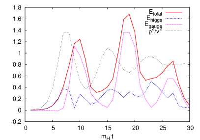
Figure 21: The analogue of figure 14: Left: $N_{\rm w}^{\rm ball}$, $N_{\rm CS}^{\rm ball}$ and $\overline{\rho^{2}}^{\rm ball}$, for a ball with a radius of 6 lattice units ($2.1\,m_{\rm H}^{-1}$) around the center of the blob. Right: excess energy, $[\int_{\rm ball}d^{3}x\,(\epsilon-\overline{\epsilon})]/E_{\rm sph}$, in the same ball and its contributions from the Higgs field and the gauge fields.

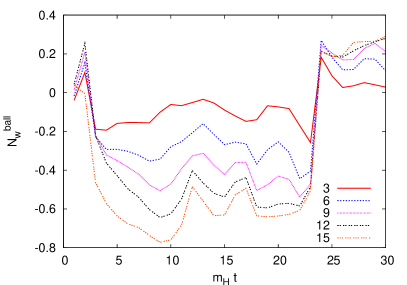
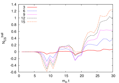
Figure 22: The analog of figure 15: $N_{\rm w}^{\rm ball}$ (left) and $N_{\rm CS}^{\rm ball}$ (right) for balls with varying radii, increasing from 3 to 15 lattice units.

Next we plot $N_{\rm w}^{\rm ball}$, $N_{\rm CS}^{\rm ball}$ and $\overline{\rho^{2}}^{\rm ball}$ for a ball of radius 6 in lattice units ($2.1m_{\rm H}^{-1}$) as a function time in the left panel of figure 21. The average Higgs length in the ball is approximately in anti-phase with the average Higgs length in the full volume, and there appears to be no damping, suggesting as in figure 14 a connection with the oscillon phenomenon [31, 32]. The winding number flips sign around $m_{\rm H}t=2$ and becomes negative. Then it makes limited excursions, even at the times where there are large peaks in $\overline{\rho^{2}}^{\rm ball}$, but between times $m_{\rm H}t=23$ and $m_{\rm H}t=24$ it makes a rapid jump by about $+0.6$, a substantial part of 1 for this relatively small ball. At this point $\overline{\rho^{2}}^{\rm ball}$ has a minimum. The Chern-Simons number of the ball does not follow the winding number very much. It shows mild negative peaks at $m_{\rm H}t=9$ and 18, shortly before the peaks in $\overline{\rho^{2}}^{\rm ball}$, and between $m_{\rm H}t=18$ and 30 it gradually increases by about 0.6 (about the same as the jump in $N_{\rm w}^{\rm ball}$ at $m_{\rm H}t=23$. In the right panel of figure 21 the total energy in the ball and the contributions from the gauge and the Higgs fields are plotted versus time. As in figure 14, we display the excess energy above the average, and with respect to the sphaleron energy. The contribution from the gauge fields is again dominant in the first two peaks (which coincide with the peaks in $\overline{\rho^{2}}^{\rm ball}$), but at $m_{\rm H}t=23$ (where $\overline{\rho^{2}}^{\rm ball}$ has a minimum) the Higgs energy clearly dominates. There is a moderate rise of the energy between $m_{\rm H}t=22$ and 27. Given that the subtracted energy is about 0.29 $E_{\rm sp}$, its maximum value is about 15% higher than the sphaleron energy. The $N_{\rm w}^{\rm ball}$ and $N_{\rm CS}^{\rm ball}$ data for balls with increasing radii are given in figure 22. The result is comparable to the early blob: both the winding number and the Chern-Simons number increase with increasing radius, indicating that there is not a sharp boundary of the blob. However, the sharp rise in $N_{\rm w}^{\rm ball}$ between $m_{\rm H}t=23$ and 24, and the steady increase of $N_{\rm CS}^{\rm ball}$ after $m_{\rm H}t=18$, are present for all ball radii.

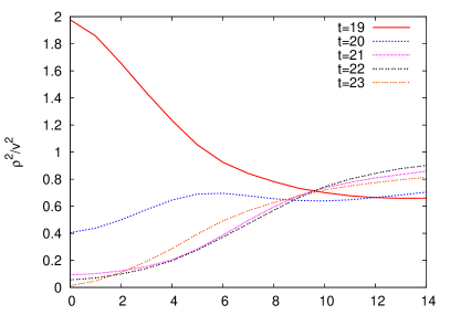
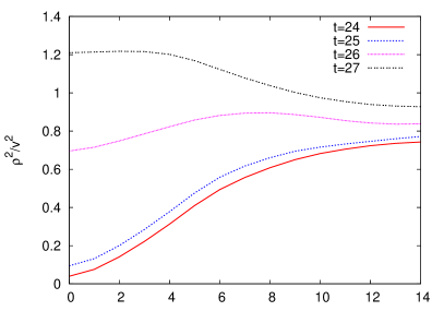
Figure 23: Profiles of the normalized Higgs length $\rho^{2}(r)/v^{2}$ for times $m_{\rm H}t=19$ to $m_{\rm H}t=23$ (left) and to $m_{\rm H}t=27$ (right). On the horizontal axis is the distance from the center $r$ in lattice units (0.35 $m_{\rm H}^{-1}$).

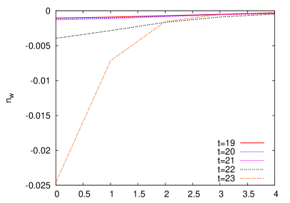
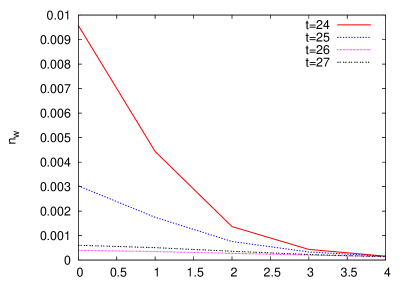
Figure 24: As in figure 23 for $n_{\rm w}(r)$.

Figures 23 and 24 show the profiles of the Higgs length and the winding number density, from times $m_{\rm H}t=19$ to $m_{\rm H}t=27$. The Higgs length at the center is decreasing and apparently developing a zero at time $m_{\rm H}t=23$, when the winding number changes, and after that it increases again. The winding profile becomes very steep around this time, as we saw also in figure 20. Lattice artefacts do not seem to be prominent in this case. Afterwards the winding density spreads and becomes very small.

The transition at $m_{\rm H}t=23$ bears the hallmarks of a sphaleron transition: a gradual $O(1)$ increase in $N_{\rm CS}$ and an $O(1)$ jump in $N_{\rm w}$, which occur locally in a blob, in the center of which $\rho$ goes through zero, together with a gradual increase in $N_{\rm CS}^{\rm bal}$ and a switch of sign in $N_{\rm w}^{\rm ball}$. The energy at that time in the ball of radius $2.1\,m_{\rm H}^{-1}$ ($1.5\,m_{W}^{-1}$) is also reasonably close to the sphaleron value ($\approx 0.9\,E_{\rm sp}$). The properties of the subsequent maximum at $m_{\rm H}t=27$ look rather similar to the two earlier ones, in its dominance of the gauge-field energy and the accompanying maxima in $\overline{\rho^{2}}^{\rm ball}$.

4.3 Distributions and susceptibilities

Here we present some quantitative results for the late distribution of winding numbers, and for the growth of the Chern-Simons susceptibility $\langle N_{\rm CS}^{2}\rangle$ during the transition. The winding-number distribution is expected to be gaussian for large volumes, but its volume dependence may contain non-trivial deviations. The rate of change of the Chern-Simons susceptibility has been interpreted as an effective sphaleron rate and used [18] to estimate the asymmetry induced by CP violation. In this section we also show results for mass ratio $m_{\rm H}=2\,m_{W}$, in addition to the value $m_{\rm H}=\sqrt{2}\,m_{W}$ used throughout this article. We vary $m_{\rm H}/m_{W}$ by varying the Higgs self coupling $\lambda$ while keeping fixed the gauge coupling $g^{2}$, the volume in Higgs mass units, $(m_{\rm H}L)^{3}$, and the lattice spacing in Higgs mass units, $am_{\rm H}$.

4.3.1 Winding distribution

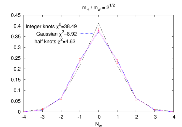
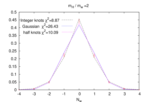
Figure 25: Normalized distribution of winding numbers at $m_{\rm H}t=30$ for $m_{\rm H}=\sqrt{2}\,m_{W}$ and $m_{\rm H}=2\,m_{W}$.

Figure 25 shows the normalized distribution of winding numbers at $m_{\rm H}t=50$ obtained from a sample of about 2000 initial conditions for each parameter set. Four fits to the data are shown as well, one based on a gaussian and three models based on a generation via winding blobs. In a first approximation we treat such blobs as being dilute and independent, which means that in a sufficiently large volume the probability for $n$ blobs is $p_{n}=cr^{n}/n!$, where $c$ is a normalization constant following from $\sum_{n}p_{n}=1$. For $n=1,2,\ldots$ this gives $c=e^{-r}$, and $r$ is the average number of blobs, which is proportional to the volume.

From a Kibble mechanism viewpoint one might expect each blob to contribute one unit to the winding number. For $n$ blobs there may be $k$ blobs contributing +1 and $n-k$ blobs contributing $-1$, such that the winding number is $N=k(+1)+(n-k)(-1)=2k-n$. Assuming a probability $a$ for +1 and $(1-a)$ for $-1$, the probability for winding number $N$ would be given by

$$P_{N}=\sum_{n=0}^{\infty}p_{n}\sum_{k=0}^{n}\left(\begin{array}[]{c}n\\ k\end{array}\right)\delta_{2k-n,N}\,a^{k}(1-a)^{n-k}=e^{-r}\left(\frac{a}{1-a}\right)^{N/2}I_{N}(2r\sqrt{a(1-a)}),$$ (42)

where $I_{N}$ is the usual Bessel function. In our case of no CP violation, $a=1/2$, and

$$P^{(1)}_{N}(r)=e^{-r}I_{N}(r).$$ (43)

For $r\gg 1$ this becomes indistinguishable from a gaussian,

$$P^{\rm gauss}_{N}(\sigma)=\frac{1}{\sqrt{2\pi\sigma^{2}}}\,e^{-N^{2}/2\sigma^{2}},$$ (44)

with $\sigma\approx r$.

However, we have argued and presented evidence that in a tachyonic quench the initial winding blobs are half-knots, some of which become stabilized by the gauge field and pick up a Chern-Simons number equal to their winding number $\pm 1/2$. So their initial winding number is conserved, although they later decay by spreading. This suggest that we modify the above model by taking into account the half integer winding of the blobs. Since the total winding number is integer, we could modify the above reasoning by assuming that in case $n$ is odd, there is a compensating contribution $\pm 1/2$ somewhere in the volume, writing $N=k(+1/2)+(n-k)(-1/2)\pm 1/2$, with equal probability 1/2 for the $\pm$ sign. The even-$n$ contribution to $P_{N}$ is unmodified. This gives

$$P^{(1/2)}_{N}(r)=e^{-r}\left[I_{2N}(r)+\frac{1}{2}I_{2N+1}(r)+\frac{1}{2}I_{2N-1}(r)\right].$$ (45)

Alternatively, we can model the compensating $\pm 1/2$ contribution by a half-knot and only allow even $n$, such that $p_{n}\to r^{n}/n!\cosh r$, which leads to the simpler form

$$P^{\prime(1/2)}_{N}(r)=I_{2N}(r)/\cosh(r).$$ (46)

The distributions $P_{N}$ are normalized, $\sum_{N=-\infty}^{\infty}P_{N}=1$.

The $\chi^{2}$ values of the fit presented in the upper plot of figure 25 for the half-knot based model of equation (46) is clearly lower than the integer model and also the gaussian model. For the model of equation (45) the result is comparable. For the lower plot the integer-knot model gives a better fit but the difference with the half-knot model is not significant ($\chi^{2}/\;{\rm d.o.f.}=1.3\;{\rm vs.}\;1.1$). This we consider additional support for the relevance of half-knots in the tachyonic transition.

4.3.2 Chern-Simons susceptibility

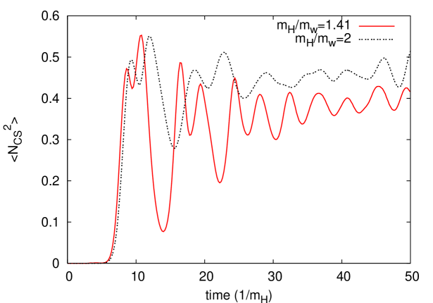
Figure 26: Chern-Simons susceptibility $\langle N_{\rm CS}^{2}(t)\rangle$ for $m_{\rm H}=\sqrt{2}\,m_{W}$ and $m_{\rm H}=2\,m_{W}$.

Figure 26 shows the time dependence of $\langle N_{\rm CS}^{2}\rangle$ for the mass ratios $m_{\rm H}/m_{W}=\sqrt{2}$ and 2. Both curves show an initial rapid rise, and the $\sqrt{2}$ case shows a deep dip near $m_{\rm H}t=13$. This is about the time where the average Higgs length also has its first minimum (actually approximately one $m_{\rm H}^{-1}$ unit later) . At this time $\int d^{3}x\,|n_{\rm w}|$ has risen again substantially (figure 8), and there is evidently no instantaneous connection with the winding number. The dip is much less pronounced (and shifted) for mass-ratio 2 case, presumably due to the stronger coupling $\lambda$, which implies a smaller initial energy density ($m_{\rm H}^{4}/16\lambda$). We have seen that the dip in the average Higgs length is also less deep in this case. This suggests fewer second-generation winding blobs, which may explain the quicker flattening of $\langle N_{\rm CS}^{2}\rangle$, compared to the $\sqrt{2}$ case. Correspondingly, the effective sphaleron rate $d\langle N_{\rm CS}^{2}\rangle/dt$ (e.g. averaged over an oscillation) will be substantial over a larger time span when $m_{\rm H}/m_{W}$ decreases.

An alternative interpretation for the first minimum in the susceptibility could be given in terms of $N_{\rm CS}$ bouncing back from a barrier in the potential of its effective equation of motion. The $\rho$-dependence of this barrier may even lead to resonant behavior [16, 19].

5 Summary and discussion

In the theory of baryogenesis the change of the Chern-Simons number of the $SU(2)$ gauge field plays an important role, and we studied the mechanism by which this can occur in a tachyonic electroweak transition. The tachyonic instability occurs initially in the Higgs field, and because of its coupling to the gauge field through the covariant derivative, one expects a correlation between the Chern-Simons number and the Higgs winding number. We argued that in a tachyonic transition there will be many places where the Higgs length is small in a typical field configuration. These places are important, since the winding number can change when the Higgs length goes through zero, possibly under influence of CP violation, and this may also induce a change in the Chern-Simons number. On the other hand, small Higgs lengths imply small Higgs currents, which may limit their influence in the equation of motion of the gauge field. Regions with small Higgs length have in general a large winding-number density, which is why we call them winding blobs.

The integrated winding number in these blobs does not need to be integer, and the basic objects have winding number close to $\pm 1/2$, the half-knots. When the dynamics causes the Higgs length to vanish in the center of a half-knot, its winding number may flip sign. Half-knot configurations occur also naturally during sphaleron transitions, and decaying textures loosing their winding number, since these have a moment at which the Higgs length vanishes at a point in space. The pure-Higgs half-knots can evaporate by increasing the Higgs length in the center, but they may also get ‘dressed’ by the gauge field adjusting its Chern-Simons number density locally to the winding. The configuration may then decay by spreading into the environmental fluctuations, and the half-knots have acted like local seeds of Chern-Simons number change.

We observed the winding blobs in numerical simulations of the tachyonic transition in the SU(2) Higgs model. Because of their large winding number density, they are easy to spot. We indeed observed a strong correlation between the half-knot winding density with the Chern-Simons number density. The picture sketched above was supported by the behavior of the integrated winding and Chern-Simons densities in small balls, as well as the radial profiles of the spherically averaged densities. Our findings for the profiles are similar to the one shown in [18].

We also analyzed an example of a realistic sphaleron transition. This occurred quite late in a blob that survived a relatively long time, showing signs of stability reminiscent of oscillons [31, 32]. In the present case we do not expect such objects to live very long as they will be destroyed by thermal fluctuations.

We found that the winding blobs can be divided into two classes. The early blobs are remnants from the initial conditions, and can sometimes survive when they are stabilized by the gauge fields. The late blobs occur when the Higgs length bounces back to small values, and there can be second, third, …, generations, especially for smaller Higgs self-couplings. Most of the early blobs are probably not important for CP violation, because interactions become important too late for them. CP violation can however affect the late blobs.

The distribution of Chern-Simons numbers is expected to be approached by the distribution of winding numbers when the volume becomes large. We studied the winding-number distribution and found that it could be fitted by models based on half-knots, better than by a model based on integer components and even marginally better than a gaussian, although for large volumes all the model-distributions are expected to become indistinguishable from a gaussian.

Finally we presented new results on the susceptibility of Chern-Simons numbers, which has been used in estimates of the baryon asymmetry [18]. Some aspects of its dependence on the Higgs self-coupling could be interpreted in terms of generations of half-knots, but a detailed understanding is difficult. Nevertheless, we expect that the increased understanding obtained in this paper is of use for modeling cold electroweak baryogenesis.

Figure 1: Parametric plot of $\phi_{2}(x)$ versus $\phi_{1}(x)$ for $x\in[-\pi,\pi]$, for the configuration of equation 16.

Figure 2: The Higgs length $\rho^{2}$ and the winding number density $n_{\rm w}$ for the configuration of equation (16) as function of $x$.

Figure 19: 3D plot for the winding number-density (upper two figures) and Chern-Simons number-density (lower two figures) at times $m_{\rm H}t=23$ (left) and $m_{\rm H}t=24$ (right).

- [1] A. D. Sakharov, Violation of CP invariance, C asymmetry, and baryon asymmetry of the universe, Pisma Zh. Eksp. Teor. Fiz. 5 (1967) 32–35.
- [2] A. G. Cohen, D. B. Kaplan, and A. E. Nelson, Progress in electroweak baryogenesis, Ann. Rev. Nucl. Part. Sci. 43 (1993) 27–70, [hep-ph/9302210].
- [3] V. A. Rubakov and M. E. Shaposhnikov, Electroweak baryon number non-conservation in the early universe and in high-energy collisions, Usp. Fiz. Nauk 166 (1996) 493–537, [hep-ph/9603208].
- [4] A. Riotto and M. Trodden, Recent progress in baryogenesis, Ann. Rev. Nucl. Part. Sci. 49 (1999) 35–75, [hep-ph/9901362].
- [5] K. Kajantie, M. Laine, K. Rummukainen, and M. E. Shaposhnikov, The electroweak phase transition: A non-perturbative analysis, Nucl. Phys. B466 (1996) 189–258, [hep-lat/9510020].
- [6] M. E. Shaposhnikov, Baryon asymmetry of the universe in standard electroweak theory, Nucl. Phys. B287 (1987) 757–775.
- [7] M. B. Gavela, P. Hernández, J. Orloff, and O. Pène, Standard model CP violation and baryon asymmetry, Mod. Phys. Lett. A9 (1994) 795–810, [hep-ph/9312215].
- [8] P. Huet and E. Sather, Electroweak baryogenesis and standard model CP violation, Phys. Rev. D51 (1995) 379–394, [hep-ph/9404302].
- [9] J. García-Bellido, D. Y. Grigoriev, A. Kusenko, and M. E. Shaposhnikov, Non-equilibrium electroweak baryogenesis from preheating after inflation, Phys. Rev. D60 (1999) 123504, [hep-ph/9902449].
- [10] L. M. Krauss and M. Trodden, Baryogenesis below the electroweak scale, Phys. Rev. Lett. 83 (1999) 1502–1505, [hep-ph/9902420].
- [11] A. D. Linde, Hybrid inflation, Phys. Rev. D49 (1994) 748–754, [astro-ph/9307002].
- [12] G. N. Felder et al., Dynamics of symmetry breaking and tachyonic preheating, Phys. Rev. Lett. 87 (2001) 011601, [hep-ph/0012142].
- [13] E. J. Copeland, D. Lyth, A. Rajantie, and M. Trodden, Hybrid inflation and baryogenesis at the TeV scale, Phys. Rev. D64 (2001) 043506, [hep-ph/0103231].
- [14] B. van Tent, J. Smit, and A. Tranberg, Electroweak-scale inflation, inflaton-Higgs mixing and the scalar spectral index, JCAP 0407 (2004) 003, [hep-ph/0404128].
- [15] J. García-Bellido, M. García Pérez, and A. González-Arroyo, Symmetry breaking and false vacuum decay after hybrid inflation, Phys. Rev. D67 (2003) 103501, [hep-ph/0208228].
- [16] J. Smit and A. Tranberg, Chern-Simons number asymmetry from CP violation at electroweak tachyonic preheating, JHEP 12 (2002) 020, [hep-ph/0211243].
- [17] J.-I. Skullerud, J. Smit, and A. Tranberg, W and Higgs particle distributions during electroweak tachyonic preheating, JHEP 08 (2003) 045, [hep-ph/0307094].
- [18] J. García-Bellido, M. García-Perez, and A. González-Arroyo, Chern-simons production during preheating in hybrid inflation models, Phys. Rev. D69 (2004) 023504, [hep-ph/0304285].
- [19] A. Tranberg and J. Smit, Baryon asymmetry from electroweak tachyonic preheating, JHEP 11 (2003) 016, [hep-ph/0310342].
- [20] J. Smit, Effective CP violation in the standard model, JHEP 09 (2004) 067, [hep-ph/0407161].
- [21] N. Turok and J. Zadrozny, Dynamical generation of baryons at the electroweak transition, Phys. Rev. Lett. 65 (1990) 2331–2334.
- [22] N. Turok and J. Zadrozny, Electroweak baryogenesis in the two doublet model, Nucl. Phys. B358 (1991) 471–493.
- [23] A. Lue, K. Rajagopal, and M. Trodden, Semi-analytical approaches to local electroweak baryogenesis, Phys. Rev. D56 (1997) 1250–1261, [hep-ph/9612282].
- [24] N. Turok, Global texture as the origin of cosmic structure, Phys. Rev. Lett. 63 (1989) 2625.
- [25] N. S. Manton, Topology in the weinberg-salam theory, Phys. Rev. D28 (1983) 2019.
- [26] F. R. Klinkhamer and N. S. Manton, A saddle point solution in the weinberg-salam theory, Phys. Rev. D30 (1984) 2212.
- [27] G. H. Derrick, Comments on nonlinear wave equations as models for elementary particles, J. Math. Phys. 5 (1964) 1252–1254.
- [28] T. Asaka, W. Buchmuller, and L. Covi, False vacuum decay after inflation, Phys. Lett. B510 (2001) 271–276, [hep-ph/0104037].
- [29] A. Arrizabalaga, J. Smit, and A. Tranberg, Tachyonic preheating using 2PI - 1/N dynamics and the classical approximation, JHEP 10 (2004) 017, [hep-ph/0409177].
- [30] G. J. Stephens, Unraveling critical dynamics: The formation and evolution of topological textures, Phys. Rev. D61 (2000) 085002, [hep-ph/9911247].
- [31] M. Broadhead and J. McDonald, Simulations of the end of supersymmetric hybrid inflation and non-topological soliton formation, Phys. Rev. D72 (2005) 043519, [hep-ph/0503081].
- [32] E. Farhi, N. Graham, V. Khemani, R. Markov, and R. Rosales, An oscillon in the SU(2) gauged Higgs model, hep-th/0505273.
- [33] J. Baacke and S. Junker, Quantum fluctuations around the electroweak sphaleron, Phys. Rev. D49 (1994) 2055–2073, [hep-ph/9308310].