Asymptotic behavior of nucleon electromagnetic form factors in time-like region

Abstract

We study the asymptotic behavior of the ratio of Pauli and Dirac electromagnetic nucleon form factors, $F_{2}/F_{1}$, in time-like region for different parametrizations built for the space-like region. We investigate how fast the ratio $F_{2}/F_{1}$ approaches the asymptotic limits according to the Phragmèn-Lindelöf theorem. We show that the QCD-inspired logarithmic behavior of this ratio results in very far asymptotics, experimentally unachievable. This is also confirmed by the normal component of the nucleon polarization, $P_{y}$, in $e^{+}+e^{-}\to N+\bar{N}$ (in collisions of unpolarized leptons), which is a very interesting observable, with respect to this theorem. Finally we observe that the $1/Q$ parametrization of $F_{2}/F_{1}$ contradicts this theorem.

I Introduction

The asymptotic behavior of the ratio $R=F_{2}/F_{1}$ of Pauli and Dirac electromagnetic nucleon form factors (FFs) has recently arised much interest from experimental and theoretical point of view. The last experimental data in space-like (SL) region Jo00 , about the momentum transfer squared ($q^{2}=-Q^{2})dependence$ of the ratio of the Sachs electric and magnetic FFs, $\mu G_{Ep}(Q^{2})/G_{Mp}(Q^{2})$ ($\mu$ is the proton magnetic moment), which has been measured with the polarization transfer method Re68 , changed the belief that the QCD asymptotic behavior of $F_{2}/F_{1}\simeq 1/Q^{2}$ Ma73 had already been reached for $Q^{2}\geq 2$ GeV² Le80 .

The recent data suggested a different behavior of this ratio: $F_{2}/F_{1}\simeq 1/\sqrt{Q^{2}}$. Such dependence has been justified in framework of different theoretical approaches Ra03 ; Ra02 ; Mi02 ; Fr96 ; Ho96 ; Ca00 ; Wa01 ; Bo02 . Another approach, confirming the QCD $1/Q^{2}$ behavior, discovered the importance of logarithmic corrections, $R\simeq ln^{2}(Q^{2}/\Lambda^{2})/Q^{2}$ Be02 , where $\Lambda$ is the soft scale related to the size of the nucleon. Note that the unexpected behavior of the ratio $\mu G_{Ep}(Q^{2})/G_{Mp}(Q^{2})$ was predicted before the experiment took place, by a particular VDM model Ia73 and also in framework of a soliton model Ho96 .

The assumption of the analyticity of FFs Dr61 allows to connect the nucleon FFs in SL and time-like (TL) regions and to study the behavior of the ratio $F_{2}/F_{1}$ in TL region. The analyticity of FFs, which has been discussed for example in Ref. Ga66 , allows to extend a parametrization of FFs available in one kinematical region to the other kinematical region.

Dispersion relation approaches Ho76 ; Du03 ; Ha04 , which are based essentially on the analytical properties of nucleon electromagnetic FFs, can be considered a powerful tool for the description of the $Q^{2}$ behavior of FFs in the entire kinematical region.

The VDM model Ia73 , after appropriate treatment of the $\rho$ contribution, can be also extrapolated from the SL region to the TL region Ia03 ; Ia04 ; Bi04 .

The quark-gluon string model Ka00 allowed firstly to find the $Q^{2}$ dependence of the electromagnetic FFs in TL region, in a definite analytical form, which can be continued in the SL region.

One of the problems concerning FFs of pions and nucleons is the large difference in the absolute values in SL and TL regions. For example, at $q^{2}$=18 GeV², the largest value at which proton TL FFs have been measured An03 , the corresponding values in TL and SL regions differ by a factor of two. The analyticity of FFs allows to apply the Phragmèn-Lindelöf theorem Ti39 which gives a rigorous prescription for the asymptotic behavior of analytical functions:

$$\lim_{t\to-\infty}F^{(SL)}(t)=\lim_{t\to\infty}F^{(TL)}(t).$$ (1)

This means that, asymptotically, FFs have the following constraints:

1. The imaginary part of FFs, in TL region, vanishes: $ImF_{i}(t)\to 0,$ as $t\to\infty$;

2. The real part of FFs, in TL region, coincides with the corresponding value in SL region: $ReF_{i}^{(TL)}(t)[t\to\infty]=F_{i}^{(SL)}(t)[t\to-\infty]$, because FFs are real functions in SL region, due to the hermiticity of the corresponding electromagnetic Hamiltonian.

The existing experimental data violate the Phragmèn-Lindelöf theorem, even at $t$ values as large as 18 GeV² ETG01 . In order to test the two requirements stated above, the knowledge of the differential cross section for $e^{+}+e^{-}\leftrightarrow p+\bar{p}$ is not sufficient, and polarization phenomena have to be studied also. In this respect, T-odd polarization observables, which are determined by $ImF_{1}F_{2}^{*}$, are especially interesting. The simplest of these observables is the $P_{y}$ component of the proton polarization in $e^{+}+e^{-}\to p+\bar{p}$ that in general does not vanish, even in collisions of unpolarized leptons Du96 , or the asymmetry of leptons produced in $p+\bar{p}\to e^{+}+e^{-}$, in the collision of unpolarized antiprotons with a transversally polarized proton target (or in the collision of transversally polarized antiprotons on an unpolarized proton target) Bi93 .

These observables are especially sensitive to different possible parametrizations of the ratio $R$, suggested by QCD and VDM models. Calculations have been done up to $t\simeq$ 40 GeV² and show that the $P_{y}$ component remains large in absolute value Br04 . For example, QCD inspired parametrizations, which fit reasonably well the data in the SL region, predict $|P_{y}|\simeq$ 35% up to $t\simeq$ 40 GeV². Such behavior has to be considered an indication that the corresponding asymptotics are very far, in agreement with the estimations of the quark-gluon string model Ka00 and VDM approach Ia03 .

Note another important property of QCD inspired predictions for nucleon FFs: the corresponding $ImF_{i}(t)$, $t\geq 4m^{2}$, $i=1,2$ ($m$ is the nucleon mass), either vanish or have a definite sign in the TL region. The previously quoted parametrizations can not apply in the whole TL region: the asymptotic pQCD behavior follows $F_{1}(t)\simeq t^{-2}$ and $F_{2}(t)\simeq t^{-3}$ at large $t$, according to the quark counting rules Ma73 . The superconvergent conditions:

$$\int_{t_{0}}^{\infty}ImF_{i}(t)dt=0,~{}i=1,2$$ (2)

has to be satisfied, where the lower limit corresponds to $t_{0}=4m_{\pi}^{2}$, for isovector FFs, and $t_{0}=9m_{\pi}^{2}$ for isoscalar FFs, where $m_{\pi}$ is the pion mass.

This implies that the nonzero QCD-contribution to Eq. (2) has to be compensated by the corresponding non-perturbative contribution of opposite sign. We can expect that such contribution mainly arises from the special region of $t$: $t_{0}\leq t\leq 4m^{2}$, which is unphysical for the process $e^{+}+e^{-}\leftrightarrow p+\bar{p}$. The contribution from the different vector mesons (with different masses) is expected to be very important here. We can say that the superconvergent condition (2) can be interpreted as a manifestation of the special duality between pQCD, from one side, and the vector meson contribution, from another side Gr74 . In principle such duality is similar to the well known Gilman-Bloom duality Bl71 , concerning the electromagnetic properties of the nucleons in SL region, when the deep inelastic electron nucleon scattering is dual to the excitation of different nucleonic resonances in $e^{-}+N\to e^{-}+N^{*}$. Also one can mention the duality in hadron physics relating the high energy behavior of the amplitudes of hadron-hadron scattering, from one side, to the resonance physics, on the other side.

Returning to the unphysical region, $t_{0}\leq t\leq 4m^{2}$, we recall, for completeness, that another interesting physical effect has to be taken into account here: a specific $\bar{N}N$ bound states, or even gluon states with $J^{PC}=1^{--}$ quantum numbers. And, due to the analyticity of FFs, these effects should appear in the SL region of momentum transfer, and should be correlated with the asymptotic behavior of FFs.

Our main aim here is to discuss the asymptotic behavior of the existing parametrizations for $F_{2}/F_{1}$ in TL region, from the point of view of the Phragmèn-Lindelöf theorem. In particular we will analyze the behavior of $Im(F_{2}/F_{1})$, its convergence to zero and study more particularly the asymptotic behavior of the $P_{y}$-component of the proton polarization in $e^{+}+e^{-}\to\bar{p}+p$, which contains equivalent information. For completeness we will also consider the behavior of the ratio ${\cal R}=|F_{2}/F_{1}|_{TL}/|F_{2}/F_{1}|_{SL}$ which should converge asymptotically to one, following the Phragmèn-Lindelöf theorem.

In order to have a quantitative estimation of the corresponding value of the relevant variable, we will use the following prescription, from Ref. Ia03 : ”A function $f(z)$ is said to be x% scaled when its value is x% of the asymptotic value $f_{as}(z)$. The value at which this condition is met is the solution of the equation $|f(z)|=x|f_{as}(z)|$ ”. For the cases considered here, this definition translates into the following three equations:

$${\cal F} = |Im(F_{2}/F_{1})|/|Re(F_{2}/F_{1})|=\Delta$$ (3)

$$|P_{y}| = \Delta~{}$$ (4)

$${\cal R} = |F_{2}/F_{1}|_{TL}/|F_{2}/F_{1}|_{SL}=1+\Delta$$ (5)

where we will take $\Delta=0.1$ and $\Delta=0.05$ in order to characterize the deviations from the asymptotic predictions of the Phragmèn-Lindelöf theorem.

For this aim, we use the following three different parametrizations, which apply in the SL region:

$$\frac{F_{2}}{F_{1}}=\displaystyle\frac{a}{\sqrt{(-t)}},~{}a=1.25\mbox{~{}GeV}\mbox{~{}from~{}Ref.~{}\cite[cite]{\@@bibref{Authors Phrase1YearPhrase2}{Br04}{\@@citephrase{(}}{\@@citephrase{)}}}},$$ (6)

$$\frac{F_{2}}{F_{1}}=0.17[\mbox{~{}GeV}^{2}]\displaystyle\frac{ln^{2}(-t/\Lambda^{2})}{(-t)}\mbox{~{}with~{}}\Lambda=0.3\mbox{~{}GeV}\mbox{~{}from~{}Ref.~{} \cite[cite]{\@@bibref{Authors Phrase1YearPhrase2}{Be02}{\@@citephrase{(}}{\@@citephrase{)}}}},$$ (7)

and the VDM inspired parametrization from Ref. Ia04 :

$$\frac{F_{2}}{F_{1}}=\displaystyle\frac{F_{2}^{(S)}+F_{2}^{(V)}}{F_{1}^{(S)}+F_{1}^{(V)}}$$ (8)

where

$$F_{1}^{(S)}(Q^{2}) = \displaystyle\frac{g(Q^{2})}{2}\left[(1-\beta_{\omega}-\beta_{\phi})+\beta_{\omega}\displaystyle\frac{\mu_{\omega}^{2}}{\mu_{\omega}^{2}+Q^{2}}+\beta_{\phi}\displaystyle\frac{\mu_{\phi}^{2}}{\mu_{\phi}^{2}+Q^{2}}\right],$$

$$F_{1}^{(V)}(Q^{2}) = \displaystyle\frac{g(Q^{2})}{2}\left[(1-\beta_{\rho})+\beta_{\rho}\displaystyle\frac{\mu_{\rho}^{2}+8\Gamma_{\rho}\mu_{\pi}/\pi}{(\mu_{\rho}^{2}+Q^{2})+(4\mu_{\pi}^{2}+Q^{2})\Gamma_{\rho}\alpha(Q^{2})/\mu_{\pi}}\right],$$

$$F_{2}^{(S)}(Q^{2}) = \displaystyle\frac{g(Q^{2})}{2}\left[(\mu_{p}+\mu_{n}-1-\alpha_{\phi})\displaystyle\frac{\mu_{\omega}^{2}}{\mu_{\omega}^{2}+Q^{2}}+\alpha_{\phi}\displaystyle\frac{\mu_{\phi}^{2}}{\mu_{\phi}^{2}+Q^{2}}\right],$$

$$F_{2}^{(V)}(Q^{2}) = \displaystyle\frac{g(Q^{2})}{2}\left[(\mu_{p}-\mu_{n}-1)\displaystyle\frac{\mu_{\rho}^{2}+8\Gamma_{\rho}\mu_{\pi}/\pi}{(\mu_{\rho}^{2}+Q^{2})+(4\mu_{\pi}^{2}+Q^{2})\Gamma_{\rho}\alpha(Q^{2})/\mu_{\pi}}\right],$$

where $g(Q^{2})=\displaystyle\frac{1}{(1+\gamma Q^{2})^{2}}$ and $\alpha(Q^{2})=\displaystyle\frac{2}{\pi}\sqrt{\displaystyle\frac{Q^{2}+4\mu_{\pi}^{2}}{Q^{2}}}ln\left[\displaystyle\frac{\sqrt{(Q^{2}+4\mu_{\pi}^{2})}+\sqrt{Q^{2}}}{2\mu_{\pi}}\right]$, with the standard values of the masses $m=0.939$ GeV, $\mu_{\rho}=0.77$ GeV, $\mu_{\omega}=0.78$ GeV, $\mu_{\phi}=1.02$ GeV, $\mu_{\pi}=0.139$ GeV and the $\rho$ width $\Gamma_{\rho}=0.112$ GeV. $\mu_{p}$ and $\mu_{n}$ are the magnetic moments of proton and neutron, respectively, whereas $\gamma=0.25$ GeV^-2, $\beta_{\rho}=0.672$, $\beta_{\omega}=1.102$, $\beta_{\phi}=0.112$, and $\alpha_{\phi}=-0.052$ are parameters fitted on the data.

This paper is organized as follows. In Section II we analyze the $t$-behavior of the imaginary part of the $F_{2}/F_{1}$ ratio for different approaches, and estimate the corresponding value of $t$ for deviations of the order of $\Delta$ from the expected asymptotic values. Then we give the expressions for the polarization observables accessible through the reaction $e^{+}+e^{-}\to p\overline{p}$ in terms of the ratio $F_{2}/F_{1}$ and analyze in particular the $P_{y}$ component of the proton polarization, which depends on the imaginary part of this ratio (Section III). In Section IV we study how the ratio ${\cal R}$ approaches to one, that is the expected value for the asymptotic regime.

II Imaginary part of the nucleon electromagnetic form factors

Let us recall here the definition of the Phragmèn-Lindelöf theorem, which will be the basis of the following discussion. Following Ti39 : if $f(z)\to a$ as $z\to\infty$ along a straight line, and $f(z)\to b$ as $z\to\infty$ along another straight line, and $f(z)$ is regular and bounded in the angle between, then $a=b$ and $f(z)\to a$ uniformly in the angle”. For the problem considered here, we identify the variable $z$ with the momentum transfer squared $t$. So one of these straight lines can be chosen along the $x$-axis, in the positive direction (in the complex $z$-plane), i.e., for $t$ values corresponding to the TL region, and the other line with negative $x$ direction, with $t$ in the SL region. Assuming the analyticity of FFs, $F_{i}(t)$, $i=1,2$, in the upper part of the $z$-plane, we satisfy the necessary conditions for the application of the Phragmèn-Lindelöf theorem, for all nucleon FFs, $F_{1,2}(t)$. More exactly, it holds also for the four independent FFs $F_{1,2}^{(S)}(t)$ and $F_{1,2}^{(V)}(t)$, where the upper indices $(S)$ or $(V)$ correspond to isoscalar or isovector electromagnetic FFs of the nucleon. Note that the analytical properties of $F_{i}(t)$, $i=1,2$, should be discussed namely for the isoscalar and the isovector FFs, and not for proton and neutron, because the unitarity conditions (which allow to calculate the imaginary part of FFs) have the simplest and most transparent form for the isotopic FFs. More exactly, isoscalar(isovector) FFs are determined by intermediate states with odd(even) number of pions.

So, finally, one can write the following four independent relations:

$$\lim_{t\to+\infty}F_{1,2}^{(S,V)}(t)=\lim_{t\to-\infty}F_{1,2}^{(S,V)}(t)$$ (9)

as a consequence of the Phragmèn-Lindelöf theorem.

This theorem has other applications in particle physics, such as, for example, the well known theorem of Pomeranchuk Lo65 , concerning the asymptotic behavior of the total cross sections for $a+b$ and $\bar{a}+b$ collisions ($a$ and $b$ any hadrons): $\sigma_{T}(ab)=\sigma_{T}(\bar{a}b)$. However, to be rigorous, the applicability of this theorem to FFs, which seems evident, has not been proved up to now.

Unfortunately, this theorem does not allow to indicate the physical value of $t$, starting from which it is working at some level of precision. For this aim one needs some additional dynamical information.

In our considerations about nucleon electromagnetic FFs, such information is contained in the parametrizations of FFs. More precisely, we discuss the ratio $F_{2}/F_{1}$ for the proton and use those parametrizations which work well in the SL region, where the available precise experimental data allow to constrain the necessary parameters. It is possible to continue analytically such parametrizations to the TL region, using the following prescription Br04 :

$$ln(-t)=ln(t)-i\pi,~{}t>0.$$ (10)

Evidently, the choice of sign for the imaginary part, in Eq. (10), results in strong physical consequences concerning the calculations of any T-odd polarization observable for $e^{+}+e^{-}\leftrightarrow N+\bar{N}$.

Let us firstly discuss the $t$-behavior of $Im(F_{2}/F_{1})$ in TL region, using the QCD inspired and VDM parametrizations. Following the Phragmèn-Lindelöf theorem, the ratio ${\cal F}=|Im(F_{2}/F_{1})|/|Re(F_{2}/F_{1})|$ should converge to zero as $t\to\infty$. And the value of $t$, corresponding to the solution of the equation: ${\cal F}=\Delta$, $\Delta\ll 1$ characterizes how ${\cal F}$ approaches to zero.

After analytical continuation in TL region, one can see that parametrization (6) gives $R\to\infty$, because it reduces in TL region to:

$$\frac{F_{2}}{F_{1}}=i\displaystyle\frac{1.25\mbox{~{}GeV}}{\sqrt{t}},~{}t>0~{}\mbox{\cite[cite]{\@@bibref{Authors Phrase1YearPhrase2}{Br04}{\@@citephrase{(}}{\@@citephrase{)}}}}.$$ (11)

Such parametrization definitely contradicts the Phragmèn-Lindelöf theorem because both form factors can not be real at the same time.

This situation is not changed, after a modification suggested to normalize FFs at $t=0$ Br04 :

$$\frac{F_{2}}{F_{1}}\to\left[\displaystyle\frac{1}{\kappa_{p}^{2}}+\displaystyle\frac{t}{(1.25)^{2}\mbox{~{}GeV}^{2}}\right]^{-1/2},$$

where $\kappa_{p}$ is the proton anomalous magnetic moment.

Parametrization (7) results in the following formula for the relative size of the imaginary to the real part ${\cal F}$:

$${\cal F}=\displaystyle\frac{2\pi~{}ln(t/\Lambda^{2})}{ln^{2}(t/\Lambda^{2})-\pi^{2}},~{}t>0,$$ (12)

which implies ${\cal F}\to 0$, if $t\to\infty$, but very slowly. Quantitatively, the condition ${\cal F}=\Delta$ has two solutions:

$$x_{\pm}=ln\displaystyle\frac{t}{\Lambda^{2}}=\displaystyle\frac{\pi}{\Delta}\left(1\pm\sqrt{1+\Delta^{2}}\right).$$ (13)

For the $x_{+}$ solution, which should be considered as the physical solution for the TL region, we obtain:

$$\sqrt{t}\simeq 10^{13}\mbox{~{}GeV},\mbox{~{}for~{}}\Delta=0.1,$$

which represents a very large energy, not far from the Planck scale, $\sqrt{t}=10^{19}$ GeV. This last value corresponds to a deviation of 6.5% from the expected asymptotical zero value.

In the model Ia73 , the isoscalar FFs, $F_{1,2}^{(S)}$, are real in all the kinematical range. Only the isovector FFs, $F_{1,2}^{(V)}$, have non vanishing imaginary part, induced by the $\rho$-meson contribution, which is, however, one order of magnitude smaller than the real part. The individual FFs are shown in Fig. 1. A singularity appears in the TL region, for all FFs, due to the dipole term and in $F_{1}^{(S)}$, due to a compensation of the $\omega$ and $\phi$ contributions.

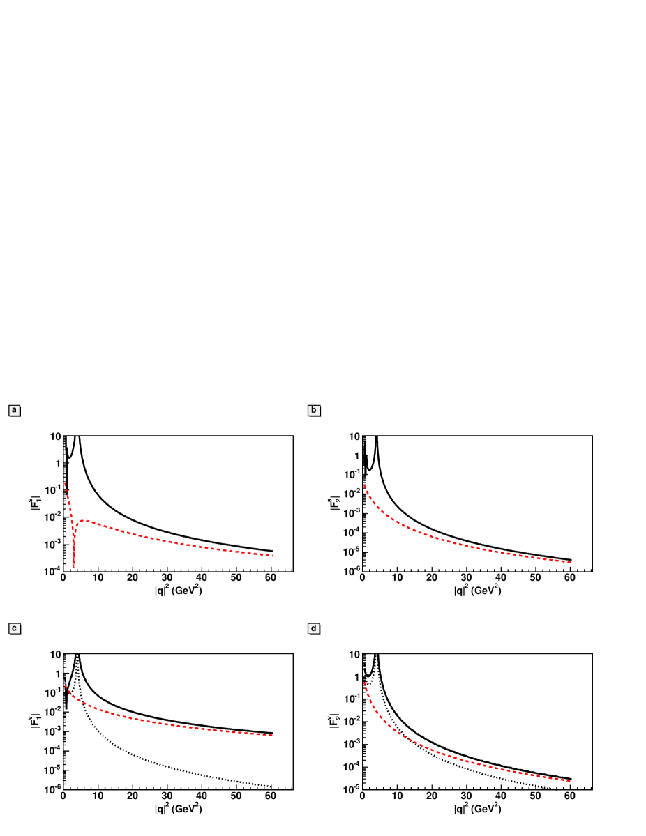
Figure 1: Isoscalar and isovector FFs in SL and TL regions. (a) and (b): $F_{1}^{(S)}$ and $F_{2}^{(S)}$ in SL region (dashed line) and in TL region (solid line), (c) and (d) $F_{1}^{(V)}$ and $F_{2}^{(V)}$ in SL region (dashed line) and in TL region: real part (solid line), imaginary part (dotted line) and absolute value (dash-dotted line) which overlaps almost everywhere with the real part.

Taking the parameters from Ref. Ia73 , one can find:

$${\cal F}=\displaystyle\frac{19.36}{[1+0.512ln(\sqrt{t}/m_{\pi})]^{2}-12.3ln(\sqrt{t}/m_{\pi})-23.5}$$ (14)

with a faster decreasing, proportional to $[ln(\sqrt{t}/m_{\pi})]^{-2}$, relatively to the previously considered parametrizations. Such asymptotic behavior leads to $\Delta$=0.1(0.05) for $\sqrt{t}=10^{11}(10^{15})$ GeV, again very far from the region experimentally accessible. Note that the contribution which is linear in logarithm as well as the constant terms in the denominator are important, as they are responsible for the zero of $Re(F_{2}/F_{1})$ at $ln(\sqrt{t}/m_{\pi})\simeq 45$, which results in a number larger than the asymptotic value.

Recently, the model Ia73 has been modified with respect to a common factor for all FFs Ia03 ; Bi04 :

$$(1-\gamma t)^{-2}\to(1-\gamma e^{i\theta}t)^{-2},$$

where $\theta$ has been taken equal to 53⁰ and $\gamma$=0.25 GeV^-2. This term moves the corresponding singularity $t=1/{\gamma}$ to $t=1/\gamma e^{i\theta}\simeq 4e^{-i\theta}$ GeV² from the physical region of TL momentum transfer. Such factor does not modify polarization phenomena as it cancels out. However, such substitution has some shortcomings as it violates the Schwartz reflection symmetry, in the following relation: $F^{*}(z)=F(z^{*})$, and does not satisfy the Phragmèn-Lindelöf theorem, because this factor induces: $ImF(t)/ReF(t)\simeq-\tan 2\theta\simeq 3.5$, i.e., a nonzero value in the asymptotic region.

III Polarization observables and asymptotic behavior of the T-odd observable $P_{y}$

Let us analyze the polarization observables related to the process $e^{+}+e^{-}\to p+\bar{p}$ and their asymptotic behavior for the considered parametrizations of $F_{2}/F_{1}$. As the $\cos\theta$ dependence is not relevant for the following considerations, for the numerical calculations we take $\theta=45^{o}$. The $\cos\theta$ dependence is well known in framework of one photon exchange Du96 , therefore, its measurement can be useful to check the validity of this mechanism at large $Q^{2}$. It is straightforward to derive the expressions for the polarization observables in terms of $F_{2}/F_{1}$ following the formalism derived in Ref. Du96 . The reference system is taken as follows: the $z$ axis along the direction of the colliding electron, the $y$ axis normal to the scattering plane, defined by the direction of the electron and of the outgoing proton, and the $x$ axis to form a left-handed coordinate system.

In case of unpolarized beam and target, only a single spin polarization observable does not vanish, the component of the polarization of the scattered proton which is normal to the scattering plane, $P_{y}$:

$$P_{y}=-\displaystyle\frac{\tau-1}{\sqrt{\tau}}\displaystyle\frac{ImF_{2}/F_{1}}{D},\\$$ (15)

where $\tau=t/(4m^{2})$ and

$$D=\displaystyle\frac{3}{2}\left|1+\displaystyle\frac{F_{2}}{F_{1}}\right|^{2}+\displaystyle\frac{1}{2\tau}\left|1+\tau\displaystyle\frac{F_{2}}{F_{1}}\right|^{2}=\displaystyle\frac{1}{2}\left[3+8Re\displaystyle\frac{F_{2}}{F_{1}}+\displaystyle\frac{1}{\tau}+(\tau+3)\left|\displaystyle\frac{F_{2}}{F_{1}}\right|^{2}\right].$$

The double spin coefficients, which do not vanish due to parity and C conservations, are:

$$A_{xx} = \displaystyle\frac{1}{2D}\left[1+\displaystyle\frac{1}{\tau}+4Re\displaystyle\frac{F_{2}}{F_{1}}+(1+\tau)\left|\displaystyle\frac{F_{2}}{F_{1}}\right|^{2}\right],$$ (16)

$$A_{yy} = \displaystyle\frac{1-\tau}{2\tau D}\left[1-\tau\left|\displaystyle\frac{F_{2}}{F_{1}}\right|^{2}\right],$$ (17)

$$A_{xz} = \displaystyle\frac{1}{\sqrt{\tau}D}\left[1+(1+\tau)Re\displaystyle\frac{F_{2}}{F_{1}}+\tau\left|\displaystyle\frac{F_{2}}{F_{1}}\right|^{2}\right],$$ (18)

$$A_{zz} = \displaystyle\frac{1}{2D}\left[3-\displaystyle\frac{1}{\tau}+4Re\displaystyle\frac{F_{2}}{F_{1}}+(3-\tau)\left|\displaystyle\frac{F_{2}}{F_{1}}\right|^{2}\right],$$ (19)

and they depend on the real part and/or on the modulus of $F_{2}/F_{1}$. The observable $P_{y}$, which contains the imaginary part of the FFs ratio, can bring information for the comparison of SL and TL asymptotic behavior.

The following formula for $P_{y}$, at $\tau\gg 1$, holds for the parametrization (6):

$$P_{y}=-\displaystyle\frac{\left(1-\displaystyle\frac{1}{\tau}\right)\displaystyle\frac{a}{m}}{3+\displaystyle\frac{1}{\tau}+\left(1+\displaystyle\frac{3}{\tau}\right)\displaystyle\frac{a^{2}}{4m^{2}}}\to P_{y,as}=-\displaystyle\frac{a/m}{3+a^{2}/(4m^{2})}\simeq-0.387.$$

This parametrization results in non vanishing (negative) asymptotics $P_{y}$, with large absolute value, in contradiction with the Phragmèn-Lindelöf theorem. The behavior of $P_{y}$ for $1/\tau\ll 1$ can be approximated by:

$$P_{y}=P_{y,as}\left(1-\displaystyle\frac{p}{\tau}\right),~{}p=1+\displaystyle\frac{3+4m^{2}/a^{2}}{1+12m^{2}/a^{2}}=1.67.$$

This implies that a 10%(5%) difference from asymptotics appears at $t=58.8(117.6)\mbox{~{}GeV}^{2}.$

For the logarithmic parametrization (7), the asymptotic behavior of $P_{y}$ is described by:

$$P_{y}\to-0.19\displaystyle\frac{ln(t/\Lambda^{2})}{\sqrt{\tau}}.$$

One can see that the absolute value decreases with $t$, and one finds $P_{y}=-10$%(-5)% at $t\simeq 350(6000)$ GeV², still too large to be achieved by experiments.

Finally, the asymptotic behavior of the $P_{y}$ polarization in the model Ia73 ; Ia03 can be described by the following formula:

$$P_{y}\to\displaystyle\frac{3.5/\sqrt{\tau}}{\left[1+0.51ln(\sqrt{t}/m_{\pi})\right]^{2}}\to\displaystyle\frac{13.5}{\sqrt{\tau}ln^{2}(\sqrt{t}/m_{\pi})}$$

with a faster decreasing with $t$. Note that this polarization is positive in TL region. Moreover the constant term in the denominator is important at large $t$, for example, a value of $P_{y}$=0.02 is reached at $t=2\cdot 10^{6}$ GeV², which corresponds to very far asymptotics.

For the cases discussed above, the large value of $|P_{y}|$ arises questions about the asymptotic trend of electromagnetic FFs. According to the prescriptions of Phragmèn-Lindelöf theorem, $P_{y}$ should vanish.

IV Difference between the absolute values of $F_{2}/F_{1}$ in SL and TL regions

We mentioned above that the measured values of the magnetic proton FFs are different in TL and SL regions of momentum transfer, up to $t=18$ GeV², where the TL values of $|G_{Mp}|^{2}$ exceed by a factor of two the corresponding values in SL region. These values should approach the same number at asymptotic values of $t$. But which number?

Let us analyze the behavior of $|F_{2}/F_{1}|$ in TL region, using, again, the considered parametrizations. The parametrization (6) gives $|F_{2}/F_{1}|_{SL}=|F_{2}/F_{1}|_{TL}$, at any value of $t$. Furthermore, this parametrization gives a specific behavior of the ratio $|G_{E}|^{2}/|G_{M}|^{2}$ in TL region. One finds:

$$\frac{|G_{E}|^{2}}{|G_{M}|^{2}}=\displaystyle\frac{1+\tau\displaystyle\frac{a^{2}}{4m^{2}}}{1+\displaystyle\frac{a^{2}}{4m^{2}\tau}}\to\tau\displaystyle\frac{a^{2}}{4m^{2}}=0.44\tau.$$ (20)

Note, in this respect, that up to now the separation of the electric and magnetic contributions to the differential cross section in the TL region has not been realized, yet. The analysis of the experimental data is currently based on two assumptions: either $G_{E}=0$ or $|G_{M}|=|G_{E}|$. The extracted values for $G_{M}$ according to these prescriptions differ at most by 20%.

However, Eq. (20) suggests another possible relation between $G_{E}$ and $G_{M}$, that leads to comparable contributions of the electric and magnetic terms to the cross section, independently on the $t$-value. The resulting value for $G_{M}$ is 10% lower than the value corresponding to $|G_{M}|=|G_{E}|$, and still does not compensate the observed difference of FFs in SL and TL regions.

The parametrization (7) gives the following relation:

$${\cal R}=\displaystyle\frac{|F_{2}/F_{1}|_{TL}}{|F_{2}/F_{1}|_{SL}}=1+\displaystyle\frac{\pi^{2}}{ln^{2}(t/\Lambda^{2})}.$$

A deviation of ${\cal R}$ from 1 by 10%(5%) is reached at $\sqrt{t}\simeq 43(337)$ GeV.

V Conclusions

We have analyzed the asymptotic behavior of recently suggested, pQCD inspired, parametrizations of the ratio of the Dirac and Pauli FFs, $F_{2}/F_{1}$. We have based our study on the requirements given by Phragmèn-Lindelöf theorem, in particular the equality of FFs in SL and TL regions. As FFs are real in SL region and complex in TL region, this implies that the imaginary part of FFs in TL region vanishes, as well as the polarization of the emitted proton, in the annihilation reaction $e^{+}+e^{-}\leftrightarrow p+\bar{p}$ (when the colliding particles are unpolarized).

We have shown that the considered parametrizations do not satisfy the asymptotic conditions suggested by the Phragmèn-Lindelöf theorem or they do so only for very large values of $Q^{2}$, well beyond the experimentally accessible range. In particular, the $1/\sqrt{Q^{2}}$ behavior of this ratio, which reproduces the recent measurements in the SL region, is certainly not compatible with an asymptotic regime, showing that the presently measurable data should be better interpreted in frame of classical nucleon degrees of freedom.

Concerning the double logarithmic parametrization, it has been pointed out long ago Mi82 , that a suppression to Sudakov type contributions could take place.

The dipole-like formulas for FFs do satisfy the Phragmèn-Lindelöf theorem. But such parametrization has the following evident problems:

• the threshold condition: $G_{EN}(4m^{2})=G_{MN}(4m^{2})$ is not satisfied,

• the unitarity conditions for all nucleon FFs are strongly violated, as one should have a branching point at $t=4m_{\pi}^{2}$ for isovector FFs and $t=9m_{\pi}^{2}$ for isoscalar FFs,

• the prediction in TL region underestimates the experimental data.

The analytical continuation of nucleon electromagnetic FFs, presently used to describe the main properties of nucleon structure in SL region of momentum transfer squared (in some models), results as a rule, in an essential imaginary part in TL region. Moreover, the relative value (with respect to the real part) is a very slowly decreasing function of $t$. Such behavior, of course, is in agreement with the Phragmèn-Lindelöf theorem, but the corresponding asymptotic regime corresponds to very large values of $t$.

The asymptotic regime defined by the prescriptions of the considered models and the asymptotic properties derived from the analyticity of form factors act at a different level. Phragmèn-Lindelöf theorem defines the asymptotic conditions without direct connection with QCD. The most evident application of the Phragmèn-Lindelöf theorem in physics is the Pomeranchuk theorem - which relates the asymptotic behavior of the total cross section for $NN$ and $N\bar{N}$ interaction. This is not QCD regime, because such theorem applies for $t=0$, i.e., to evidently non perturbative physics, despite the fact that the Mandelstam variable $s$ is very large. So the connection between QCD asymptotics and asymptotics from Phragmèn-Lindelöf theorem, from the point of view of hadron FFs is non trivial, as this theorem seems to work for elastic $NN$ and $N\bar{N}$ amplitudes in the kinematical region where QCD does not apply.

We can consider the present results as an indirect indication of the importance of non perturbative contributions to the physics of the nucleon electromagnetic structure.

VI Acknowledgments

The authors acknowledge Prof. M. P. Rekalo for many interesting discussions and ideas, without which this paper would not have been realized in the present form. Thanks are due to Prof. E. Kuraev for his interest to this subject and to C. Duterte for contributing to the earlier stage of this work.

References

- (1) M. K. Jones et al., Phys. Rev. Lett. 84, 1398 (2000); O. Gayou et al., Phys. Rev. Lett. 88, 092301 (2002).
- (2) A. Akhiezer and M. P. Rekalo, Dokl. Akad. Nauk USSR, 180, 1081 (1968); Sov. J. Part. Nucl. 4, 277 (1974) [Fiz. El. Chast. Atom. Yad. 4, 662 (1973)].
- (3) V. Matveev et al., Nuovo Cimento Lett. 7, 719 (1973).
- (4) G. P. Lepage and S. J. Brodsky, Phys. Rev. D 22, 2157 (1980); S. J. Brodsky and G. P. Lepage, Phys. Rev. D 24, 2848 (1981).
- (5) J. P. Ralston and P. Jain, Phys. Rev. D 69, 053008 (2004).
- (6) J. P. Ralston, P. Jain and R. V. Buniy, AIP Conf. Proc. 549, 302 (2000).
- (7) G. A. Miller and M. R. Frank, Phys. Rev. C 65, 065205 (2002).
- (8) M. R. Frank, B. K. Jennings and G. A. Miller, Phys. Rev. C 54, 920 (1996).
- (9) G. Holzwarth, Z. Phys. A 356, 339 (1996).
- (10) F. Cardarelli and S. Simula, Phys. Rev. C 62, 065201 (2000).
- (11) R. F. Wagenbrunn, S. Boffi, W. Klink, W. Plessas and M. Radici, Phys. Lett. B 511, 33 (2001).
- (12) S. Boffi, L. Y. Glozman, W. Klink, W. Plessas, M. Radici and R. F. Wagenbrunn, Eur. Phys. J. A 14, 17 (2002).
- (13) A. V. Belitsky, X. d. Ji and F. Yuan, Phys. Rev. Lett. 91, 092003 (2003).
- (14) F. Iachello, A. D. Jackson and A. Lande, Phys. Lett. B 43 (1973) 191.
- (15) S. D. Drell and F. Zachariasen, ’Electromagnetic Structure of nucleons’, Oxford University Press, 1961.
- (16) S. Gasiorowicz, ’Elementary Particle Physics’, John Wiley and Sons, Inc. 1966.
- (17) G. Hohler, E. Pietarinen, I. Sabba Stefanescu, F. Borkowski, G. G. Simon, V. H. Walther and R. D. Wendling, Nucl. Phys. B 114, 505 (1976); G. Hohler and E. Pietarinen, Phys. Lett. B 53, 471 (1975).
- (18) H.W. Hammer and Ulf-G. Meissner, Eur. Phys. J. A 20, 469 (2004).
- (19) S. Dubnicka, A. Z. Dubnickova, and P. Weisenpacher, J. Phys. G. 29, 405 (2003); S. Dubnicka, A. Z. Dubnickova, arXiv:hep-ph/0401081.
- (20) F. Iachello, arXiv:nucl-th/0312074.
- (21) F. Iachello and Q. Wan, Phys. Rev. C 69, 055204 (2004).
- (22) R. Bijker and F. Iachello, Phys. Rev. C 69, 068201 (2004).
- (23) A. B. Kaidalov, L. A. Kondratyuk and D. V. Tchekin, Phys. Atom. Nucl. 63, 1395 (2000) [Yad. Fiz. 63, 1474 (2000)].
- (24) M. Andreotti et al., Phys. Lett B 559, 20 (2003).
- (25) E. C. Titchmarsh, Theory of functions, Oxford University Press, London, 1939, p. 179.
- (26) E. Tomasi-Gustafsson and M. P. Rekalo, Phys. Lett. B 504, 291 (2001) and refs herein.
- (27) A. Z. Dubnickova, S. Dubnicka and M. P. Rekalo, Nuovo Cim. A 109, 241 (1996).
- (28) S. M. Bilenkii, C. Giunti and V. Wataghin, Z. Phys. C59, 475 (1993).
- (29) S. J. Brodsky, C. E. Carlson, J. R. Hiller and D. S. Hwang, Phys. Rev. D 69, 054022 (2004).
- (30) D. J. Gross and S.B. Treiman Phys. Rev. Lett. 32, 1145 (1974).
- (31) E. D. Bloom and F. J. Gilman, Phys. Rev. D 4, 2901 (1971).
- (32) A. A. Logunov, N. van Hieu and I. T. Todorov, Annals of Physics 31, 203 (1965).
- (33) T. Gousset and B. Pire, Phys. Rev. D 51, 15 (1995).
- (34) A. P. Bakulev, A. V. Radyushkin and N. G. Stefanis, Phys. Rev. D 62, 113001 (2000).
- (35) A. I. Milshtein and V. S. Fadin, Yad. Fiz. 35 (1982) 1603.