Statistically improved Analysis of Neutrino Oscillation Data with the latest KamLAND results

We present an updated analysis of all available solar and reactor neutrino data, emphasizing in particular the totality of the KamLAND (314d live time) results and including for the first time the solar $SNO$ (391d live time, phase II NaCl-enhanced) spectrum data. As a novelty of the statistical analysis, we study the variability of the KamLand results with respect the use of diverse statistics. A new statistic, not used before is proposed. Moreover, in the analysis of the SNO spectrum a novel technique is used in order to include full correlated errors among bins. Combining all data, we obtain the following best-fit parameters: we determine individual neutrino mixing parameters and their errors $\Delta m^{2}=8.2\pm 0.08\times 10^{-5}{\rm eV}^{2},\quad\tan^{2}\theta=0.50^{+0.12}_{-0.07}.$ The impact of these results is discussed. We also estimate the individual elements of the neutrino mass matrix. In the framework of three neutrino oscillations we obtain the mass matrix:

$$M = eV\pmatrix{1.0+4.0\pm 3.2\ 10^{-5}&4.2\pm 3.2\ 10^{-5}&-13.5\pm 14.0\ 10^{-5}\cr 4.2\pm 3.2\ 10^{-5}&1.0+4.3\pm 3.5\ 10^{-5}&-13.5\pm 14.5\ 10^{-5}\cr 13.5\pm 14.0\ 10^{-5}&-13.5\pm 14.5\ 10^{-5}&1.0+100.0\pm 30.0\ 10^{-5}}.$$

1 Introduction

Evidence of antineutrino disappearance in a beam of antineutrinos in the Kamland experiment has been presented klJun . The analysis of previous experimental results on reactor physics and solar neutrinos klothers in terms of neutrino oscillations has largely improved our knowledge of neutrino mixing. Thus, the solar neutrino data evidence prior to autumn of 2003 converged to two distinct allowed regions in parameter space, often referred to as LMAI (centered around the best-fit point of $\Delta m^{2}_{\odot}=7.1\times 10^{-5}{\rm eV}^{2}$, $\tan^{2}\theta_{\odot}=0.47$) and LMAII (centered around $\Delta m^{2}_{\odot}=1.5\times 10^{-4}{\rm eV}^{2}$, $\tan^{2}\theta_{\odot}=0.48$). The inclusion of SNO phase II data eliminated the LMAII region at about $4\sigma$.

The KamLAND measurementes presented recently klJun corresponds to the first about 317 days live time, they confirm the conclusions obtained from previous data and give a more stringent limit on the neutrino mass parameters. As we will see in this work, the new KamLAND information further excludes the LMAII region now at $\approx$ 5$\sigma$.

In addition to an increased statistics, a significant change in the KamLAND analysis technique is related to the fiducial volume definition. Whereas in the previous setup, events taking place at the outer edge of the nylon balloon were rejected klJun ; Eguchi:2002dm , the recent analysis adopts a more sophisticated coincidence-measurement technique to exclude unwanted backgrounds. Additionally, a better understanding of the fuel cycle on the reactors has lead to the collaboration to estimate the incoming neutrino flux with better accuracy: the estimated error on this initial flux $\phi_{0}\left(\overline{\nu}_{e}\right)$ is now of the order of 2%.

The aim of this work is to present a comprehensive updated analysis of all recent solar neutrino data including the KamLAND reactor-experiment results to determine the extent of the remaining viable region in the parameter space and to obtain favoured values for the neutrino physical parameters in a two-neutrino framework, and, with the inclusion of results coming from atmospheric oscillation evidence give an estimation of the elements of the three neutrino mass matrix. Some key analysis novelties are presented along this work, for example regarding the treatment of sistematic correlations in the analysis of the SNO spectrum (day+night) and a improved analysis of the KL data with an appropriate consideration of its low statistics data bins.

The structure of this paper is the following: in section 2 discuss our approach to the latest KamLAND results and older solar evidence. All solar neutrino experiments are discussed in section 2.1. We specially discuss the importance of the SNO data and the spectrum results. We then proceed, in section 3, to explain the procedure adopted in our analysis with some emphasys on the special treatment needed by the KamLand and SNO spectra and in section 4 we present our results. Finally we summarize and conclude in section 5.

2 The KamLAND and solar evidence

Reactor anti-neutrinos with energies above 1.8 MeV produced in some 53 commercial reactors are detected in the KamLAND detector via the inverse $\beta$-decay reaction $\overline{\nu}_{e}+p\rightarrow n+e^{+}$. The mean reactor-detector distance and energy window of these $\overline{\nu}_{e}$ makes KamLAND an ideal testing ground for the LMA region of the $\nu_{\odot}$ parameter space. The first results published by the KamLAND collaboration eliminated all possible solutions to the solar neutrino problem (SNP) except the LMA region of the parameter space Eguchi:2002dm . The sensitivity of this experiment to the $\Delta m^{2}$ parameter divided the previously whole LMA region into two distinct regions, the one relative to the smaller mass-squared difference being preferred by data postKamland .

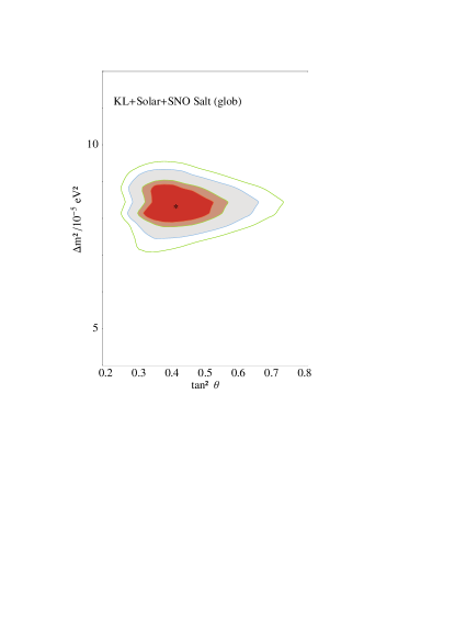
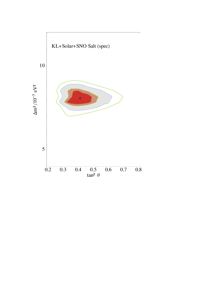
Figure 1: (left) Allowed region in the $(\tan^{2}\theta,\Delta m_{\odot}^{2})$ plane for the global analysis, which includes the previous solar data (see e.g. ourstuff for details) and all KamLAND Global results. (right) Best fit solution for the spectrum analysis, including all previous solar data, short baseline reactor data and the KamLAND spectrum. Best fit point given in table [4].

In our analysis (see also Ref.torrente for further details) we model the reactor incoming flux through a constant, time-averaged fuel composition for all of the commercial reactors within detectable distance of the Kamioka site, namely ${}^{235}\text{U}=56.3\%$, ${}^{238}\text{U}=7.9\%$, ${}^{239}\text{Pu}=30.1\%$, and ${}^{241}\text{Pu}=5.7\%$. We used the full cross-section including electron recoil corrections. We analyzed the data above threshold of $2.6{\rm MeV}$, as the low-energy end of the spectrum had effectively no events. The information relative to the no-oscillation initial flux for the two periods can be extracted from fig. (1.a) of klJun . We neglect all backgrounds, including geological background above 2.6 MeV. We use the resolutions published by the collaboration for the two different data sets, namely $\sigma\left(E\right)=6.2\%/\sqrt{E}$ for the recent data (post upgrade) and $\sigma\left(E\right)=7.3\%/\sqrt{E}$ for earlier data (pre-upgrade). The total systematic error is estimated at $6.5\%$.

In order to use all the data available, we use a simple MC simulation to estimate an equivalent efficiency for the two pre-upgrade and post-upgrade phases. Finally, no matter effects are taken into consideration for the KamLAND data alone, as it was shown that, for this experiment, any asymmetry due to matter effects is negligible for $\Delta m^{2}$ of the order of $10\times 10^{-5}$ eV².

2.1 Solar data

The most ponderous data present in our analysis come from the solar neutrino experiments. The experimental results are compared to an expected signal which we compute numerically by convoluting solar neutrino fluxes bpb2001 , sun and earth oscillation probabilities, neutrino cross sections and detector energy response functions. We closely follow the same methods already well explained in previous works Aliani:2001zi ; Aliani:2001ba ; Aliani:2002ma ; Aliani:2002rv , we will mention here only a few aspects of this computation. We determine the neutrino oscillation probabilities using the standard methods found in literature torrente , as explained in detail in Aliani:2001zi and in Aliani:2002ma . We use a thoroughly numerical method to calculate the neutrino evolution equations in the presence of matter for all the parameter space. For the solar neutrino case the calculation is split in three steps, corresponding to the neutrino propagation inside the Sun, in the vacuum (where the propagation is computed analytically) and in the Earth. We average over the neutrino production point inside the Sun and we take the electron number density $n_{e}$ in the Sun by the BPB2001 model bpb2001 . The averaging over the annual variation of the orbit is also exactly performed. To take the Earth matter effects into account, we adopt a spherical model of the Earth density and chemical composition torrente . The joining of the neutrino propagation in the three different regions is performed exactly using an evolution operator formalism torrente . The final survival probabilities are obtained from the corresponding (non-pure) density matrices built from the evolution operators in each of these three regions.

In summary, double-binned day-night and zenith angle bins are computed in order to analyze the full SuperKamiokande data Smy:2002fs , whereas single-binned data is used for the SNO detector newSNO ; Poon:2001ee ; Ahmad:2002jz . The global signals only are used for the radiochemical experiments Homestake homestake , SAGE sage1999 ; sage , GallEx gallex and GNO gno2000 . The next paragraphs are dedicated to a description of SNO component of the solar evidence.

The Sudbury Neutrino Observatory (SNO) collaboration has presented data relative to the NaCl phase of the experiment newSNO ; newSNO03 . We remind that the addition of NaCl to a pure $\text{D}_{2}\text{O}$ detection medium has the effect of increasing the detector’s sensitivity to the neutral-current (NC) reactions within its fiducial volume. The NC detection efficiency has changed from a previous ’no-salt’ phase of approximately a factor three. This and other novelties have made it possible for the SNO collaboration to analyze their data without making use of the no-spectrum-distortion hypothesis. Furthermore, they have adopted a new ’event topology’ criterion newSNO03 to distinguish among the different channels within the detector. The SNO Collaboration has now devised a new data-analysis technique which relies on the topology of the three different events. The new parameter ($\beta_{\ell}$) relative to which they marginalize is known as the ’isotropy’ of the Cerenkov light distribution was used to separate the CC, ES and NC signals, something that was not possible in th previous two data sets. The measured fluxes are reported in newSNO .

The comparison of the new SNO results and the previous phase-II data can easily be made because the SNO collaboration has included in the recent paper results which were obtained following their previous method, along with the new unconstrained data. The new results are compatible with the previous ones. It seems that the overall effect of un-constraining the analysis is an increase in the measured fluxes, although the estimated total $\Phi_{\text{B}}$ has decreased relative to the previous best-fit value, leaving even less space for eventual sterile neutrinos. We make use of all day+night published data and refer the reader to section 3 for details. The procedure we used to introduce the SNO spectrum data is an extention of the one use for the SK spectrum analysis and is explained in the next section.

3 Our analysis

We use standard statistical techniques to test the non-oscillation hypothesis. Two different sets of analyses are possible with the present data on neutrino oscillations: 1) short-baseline reactor data, solar data including the SK spectrum and previous phase-I (CC only) SNO spectrum, phase-II SNO global result, combined with new the KamLAND spectrum and, 2) the previous set with the use of the phase-II SNO spectrum result and the new KamLAND data. In order to use all the SNO data, we consider the phase-I and phase-II results as two distinct but fully correlated experiments.

For the purpose of this analysis, a $\chi^{2}$ function is defined which is the the sum of the distinct contributions. The contribution of all solar neutrino experiments is summarized in the term:

$$\chi^{2}_{sun}=\chi_{rad}+\chi_{SK}^{2}+\chi^{2}_{\text{SNO}}.$$ (1)

Where, the $\chi^{2}$ function for the global rates of the radiochemical experiments is as follows,

$$\chi^{2}_{\text{rad}}=\left(\mathbf{R}^{\text{th}}-\mathbf{R}^{\text{exp}}\right)^{T}\left(\sigma_{\text{sys}}+\sigma_{\text{stat}}\right)^{-1}\left(\mathbf{R}^{\text{th}}-\mathbf{R}^{\text{exp}}\right),$$ (2)

where $\mathbf{R}^{\text{th,exp}}$ are length-two vectors containing the theoretical (or experimental) signal-to-no-oscillation expectation for the chlorine and gallium experiments. Correlated systematic and uncorrelated statistical errors are considered in $\sigma_{\text{syst}}$ and $\sigma_{\text{stat}}$ respectively. Note that the parameter-dependent $R^{\text{th}}$ is an averaged day-night quantity, as the radiochemical experiments are not sensitive to day-night variations. For the next component We consider the double-binned SK spectrum comprising of 8 energy bins for a total of 6 night bins and one day bin. The $\chi^{2}$ is given by

$$\chi^{2}_{\text{SK}}=(\alpha\mathbf{R}^{\text{th}}-\mathbf{R}^{\text{exp}})^{T}\left(\sigma^{2}_{\text{unc}}+\sigma^{2}_{\text{cor}}\right)^{-1}(\alpha\mathbf{R}^{\text{th}}-\mathbf{R}^{\text{exp}}).$$ (3)

The covariance matrix $\sigma$ is a 4-rank tensor containing information relative to the statistical errors and energy and zenith-angle bin-correlated and uncorrelated uncertainties. Since the publication of the first SNO NC results, we have adopted their estimate of $\phi_{B}$ and incorporated the new parameter $\alpha$ in the $\chi^{2}$ representing the normalization with respect to this quantity. In determining our best-fit points, we minimize with respect to it. Note that the quantities $\mathbf{R}^{\text{exp}}$ and $\mathbf{R}^{\text{th}}$ contain the number of events normalized to the no-oscillation scenario.

We deal next with the SNO component. We present two different analysis of some of the phase II SNO data sets including total day/night quantities.

The first consideres the global signal alone, the second incorporates the total signal spectrum. We consider here the two SNO results as if coming from two independent experiments, but fully correlated. We use the backgrounds as listed in tables X of Ref.newSNO and 1 of Ref.Ahmad:2002jz for the phase-II data. The detector resolution is obtained from Refs. newSNO ; howto .

In the second case we make use of the spectral data. The spectrum used for our analusis is presented in table [2]). The $\chi_{\text{SNO}}^{2}$ has the same formal expression as before, where it is understood that $\mathbf{R}^{\text{th,exp}}$ are now length 32 containing two 16-bin relative to the two SNO data sets. We consider the two fully correlated.

The main difficulty in using the total spectrum data lies in correctly estimating the, highly correlated, systematic error. By using the information contained in tables XIX and XX of Ref.newSNO , we have computed the influence of all the different sources of error on our response function considering the correlation/anti-correlation as presented in table 1 of howto . The different backgrounds spectral correlations are included from table XXXIV of Ref.newSNO . The procedure we used to introduce the SNO spectrum data is an extension of the one used for the SK spectrum analysis. For each point in the parameter space $\Delta m^{2}$, $\theta$ we start from a correlation matrix obtained by using the non-deformed spectrum assumption. We calculate, for each bin, the sum of the signals ES+NC+CC and we extract weights for each single contributions. After that, we compare our theoretical results with the ones given by the SNO collaboration and impose a 3-$\sigma$ cut. By using these zero-order weights and the correlation errors obtained by the SNO table, we reconstruct a correlation matrix. The correlation matrix is introduced into the $\chi^{2}$ analysis by adding a free parameter $\delta_{cor}$ which is determined in a minimization process togethed with the weights of the single $i=ES+NC+CC$ contributions to the signal:

$$\chi^{2}_{SNO} = \sum_{i}(\alpha R^{th}-R^{exp})^{t}(\sigma^{2}_{unc}+\delta_{cor}\sigma^{2}_{cor})^{-1}(\alpha R^{th}-R^{exp})$$

$$+\chi^{2}_{\alpha}+\chi^{2}_{\delta_{cor}},$$

The full process is designed to be interated a number of times, in practise we obtain that after two iterations the process is convergent and give us the desired results.

3.1 The Kamland statistical analysis

The total KamLAND contribution to the $\chi^{2}$ is defined as:

$$\chi^{2}_{\text{KL}}=\chi^{2}_{\text{KL,glob}}+\chi^{2}_{\text{KL},\lambda}$$ (4)

where the global contribution is simply

$$\chi^{2}_{\text{KL,glob}}=\frac{\left(R^{\text{th}}-R^{\text{exp}}\right)^{2}}{\sigma_{\text{stat+sys}}^{2}}.$$ (5)

The statistical consideration of the KL spectrum signal, $\chi^{2}_{KL,\lambda}$, is however worthy of special attention. Due to the fact that at high energy KamLAND observes a small number of events alternatives should be used instead the Gaussian approximation. This means among other things that the correlated systematic deviations cannot be introduced in a straightforward way. Due to these reasons, we use an alternative technique for the KamLAND data bins. A detailed account of some statistical considerations is presented in the Appendix.

It is possible to present an unified approach read88 to all the commonly used multinomial models (Pearson’s, log-likelihood among them) by defining a family of statistics $\chi^{2}(\lambda)$ for testing the fit of observed frequencies $R_{i}^{exp}$ to the expected ones $R_{i}^{th}$ read88 . All the statistics belonging to this family have similar well-behaved properties but however results as best fit parameters and exclusion regions may significantly depend on the use of one or another. Any decision as to which member of the family we should use to finally test the null hypothesis must depend on the type of the departure we wish to detect. The sensitivity of the statistic depends on how the defining function treats the large or small deviations.

Based on a comparative study it is recomended read88 ; stat to use $\chi^{2}(2/3)$ as a compromise candidate among the different test statistics optimizing diverse criteria as rate of convergence, sensitivity to the sample size and sensitivity to large or small bin deviations. The statistic corresponding to this value, the Read statistic, is the one used in this work:

$$\chi^{2}_{KL}\left(\lambda=\frac{2}{3}\right) = \frac{9}{5}\sum_{i}R_{i}^{exp}\left(\left(\frac{R_{i}^{exp}}{R_{i}^{th}}\right)^{2/3}-1\right)$$

$$+\frac{2}{3}\left(R_{i}^{th}-R_{i}^{exp}\right).$$

In the evaluation of $\chi^{2}_{\text{KL},\lambda}$ we use vectors that comprise therefore of 13 spectral points of width 0.425 MeV.

4 Results and Discussion.

To test a particular oscillation hypothesis against the parameters of the best fit (null hypothesis) and obtain allowed regions in parameter space we perform a minimisation of the full function $\chi^{2}$ with respect the oscillation and the rest of ancillary parameters. A given point in the oscillation parameter space is allowed if the globally subtracted quantity fulfills the condition $\Delta\chi^{2}=\chi^{2}(\Delta m^{2},\theta)-\chi_{\rm min}^{2}<\chi^{2}_{n}(CL)$. Where $\chi^{2}_{(}90\%,95\%,...)$ are the respective quantiles. In this way we obtain best fit mass differences and angles and joint exclusion regions. Additionally, we perform a second kind of analysis in order to obtain concrete values for the individual oscillation parameters and estimates for their uncertainties. We study the marginalised parameter constraints where the $\chi^{2}$ quantity is converted into likelihood using the expression ${\cal L}/{\cal L}_{0}=$ $e^{-(\chi^{2}-\chi_{min}^{2})/2}$.

In table [4] we report the values of the mixing parameters $\Delta m^{2}_{\odot}$, $\tan^{2}\theta_{\odot}$, and the $\chi^{2}$ obtained from minimization and from the peak of marginal likelihood distribution.

The results are shown in Figs.1 where we have generated acceptance contours in the $\Delta m^{2}$-$\tan^{2}\theta$ plane. In fig. [1-(left)] we show the exclusion plots for the solar, radiochemical + Cerenkov solar data and KamLAND with the global signal of the SNO phase-II data, whereas the right panel refers to the KamLAND spectrum, radiochemical + Cerenkov solar data and the SNO phase-II spectrum information. Contour lines correspond to the the allowed areas at 90, 95, 99 and 99.7% CL relative to the absolute minimum.

Thes normalized marginal likelihood, obtained from the integration of ${\cal L}$ for each of the variables, is plotted in Figs. (2) for each of the oscillation parameters $\Delta m^{2}$ and $\tan^{2}\theta$. Concrete values for the parameters are extracted by fitting one- or two-sided Gaussian distributions to any of the peaks (fits not showed in the plots). In both cases, for angle and the mass difference distributions the goodness of fit of the Gaussian fit to each individual peak is excellent (g.o.f $\sim 100\%$). The errors obtained from this method are assigned to the $\chi^{2}$ minimisation values. The central values are fully consistent and very similar to the values obtained from simple $\chi^{2}$ minimisation. Systematics variability of these results can come from the use of a different prior information or mixing parameterizations, however this variability or systematic error due to the procedure is small. We will again use the technique of marginal distributions in the next paragraphs to obtain an estimation of the individual elements of the neutrino mass matrix and their errors.

The main difference with previous analysis is a better resolution in parameter space. The previously two well separated solutions LMAI,LMAII have now completely disappeared. In particular the secondary region at larger mass differences (LMAII) is now completely excluded.

The introduction of the new KamLand data in general strongly diminishes the favored value for the mixing angle with respect to the KamLAND result alone Aliani:2002na . The final value is more near to those values favored by the solar data alone than to the KamLAND ones. As an important consequence, the combined analysis of solar and KamLAND data concludes that maximal mixing is not favored at $\sim 4-5\sigma$. This conclusion is not supported by the antineutrino, earth-controlled, conceptually simpler KamLAND results alone. As we already pointed out in Ref.Aliani:2002na , this effect could be simply due to the present low KamLAND statistics or, more worrying, to some statistical artifact derived from the complexity of the analysis and of the heterogeneity of binned data involved.

4.1 An estimation of the neutrino mass matrix

We proceed now to an estimation of the neutrino mass matrix in different aproximations. Our main objective is however to estimate how well the individual errors of the mass matrix can be extracted already at present by the existing experimental evidence. For this purpose we have applied similar arguments as those used before to obtain marginal distributions and errors for individual parameters from them.

The square of the neutrino mass matrix can be written in the flavour basis as $M^{2}=UM_{D}^{2}U^{\dagger}$ where $M_{D}$ is diagonal and $U$ is an unitary (purely active oscillations are assumed) mixing matrix. Subtracting one of the diagonal entries we have

$$M^{2}=m_{1}^{2}I+M_{0}^{2}=m_{1}^{2}I+UM_{D}^{\prime 2}U^{\dagger},$$

where $I$ is the identity matrix. In this way we distinguish in the mass matrix a part, $M_{0}^{2}$, which affects and can be determined by oscillation experiments and another one, $m_{1}^{2}I$, which does not. Evidently, the off-diagonal elements of the mass matrix are fully measurable by oscillation experiments.

First, we restric ourselves for the sake of simplicity to two neutrino oscillations, we have in this case

$$M^{2}=m_{1}^{2}I+M_{0}^{2} = m_{1}^{2}I+\Delta m^{2}\pmatrix{\sin^{2}\theta&\sin\theta\cos\theta\cr\sin\theta\cos\theta&\cos^{2}\theta}$$ (6)

with $\Delta m^{2}=m_{2}^{2}-m_{1}^{2}$. The individual elements of the matrix $M_{0}$ can simply be estimated from the oscillation parameters obtained before. For example for $\tan^{2}\theta\sim 0.40$, $\Delta m^{2}\sim 7-8\times 10^{-5}\ eV^{2}$ we would obtain $(M_{0}^{2})_{22}\sim 5-6\times 10^{-5}\ eV^{2}$.

Using again as likelihood function the quantity lkadlk ${\cal L}/{\cal L}_{0}(\Delta m^{2},\tan^{2}\theta)=$ $e^{-(\chi^{2}-\chi_{min}^{2})/2}$ we obtained the individual probability distributions for any of the elements of the matrix $M_{0}$. Average values and $1\sigma$ errors are obtained from two-sided Gaussian fits to these distributions. From this procedure we obtain:

$$M_{0}^{2} = 10^{-5}\ eV^{2}\pmatrix{2.05^{+0.25}_{-0.26}&3.12^{+0.25}_{-0.26}\cr 3.12^{+0.25}_{-0.26}&4.50^{+0.51}_{-0.40}}.$$ (7)

One can go further supposing a concrete value for $m_{1}^{2}$ from elsewhere. If we take $m_{1}^{2}>>\Delta m^{2}$ then we can directly write the mass matrix

$$M = m_{1}I+\frac{1}{2m_{1}}M_{0}^{2}.$$ (8)

Supposing for example $m_{1}=1\ eV$,

$$M = eV\pmatrix{1.0+1.02^{+0.12}_{-0.12}\ 10^{-5}&1.56^{+0.12}_{-0.13}\ 10^{-5}\cr 1.56^{+0.12}_{-0.13}\ 10^{-5}&1.0+2.25^{+0.25}_{-0.20}\ 10^{-5}}.$$

this is the final two neutrino mass matrix which can be obtained from present oscillation evidence coming from solar and reactor neutrinos.

We obtain now an estimation of the three neutrino mass matrix. For this purpose we make the same reasoning as before and introduce the existing evidence of the individual values of the two additional angles and the square mass difference. Naturally knowledge of these parameters is still very poor and the elements of the final mass matrix will have much larger errors. First we substract a diagonal part and write the square mass matrix $M^{2}$ as:

$$M^{2}=m_{2}^{2}I+M_{0}^{2} = m_{2}^{2}I+\Delta m^{2}_{12}M_{12}^{2}+\Delta m^{2}_{32}M_{32}^{2}$$

with $\Delta m^{2}_{ij}=m_{i}^{2}-m_{j}^{2}$.

We write the mixing matrix as a product of three single rotations around each of the axis:

$$U=u_{12}(\theta_{12})u_{23}(\theta_{23})u_{13}(\theta_{13}).$$

With this notation the matrices $M_{12},M_{32}$ are written

$$M_{12}=(u_{23}u_{13})^{t}M_{0}^{2}u_{23}u_{13},$$

$$M_{32}=(u_{23}u_{13})^{t}M_{3}u_{23}u_{13}$$

where $M_{3}=Diag(0,0,1)$. The matrix $M_{32}$ does not depend on the angle $\theta_{12}$. The dependence on this angle is fully contained in $M_{0}$ which is the $3\times 3$ enlarged version of the $M_{0}$ matrix appearing in Eqs.(6,7).

We take the best values for $\Delta m_{32}$ known at present (see for example Ref.neutrinos3 and references therein) and from CHOOZ evidence chooznew ; PaloVerde the value of the $(13)$ angle: $1.3\,\times\,10^{-3}\,\mbox{eV}^{2}\,\leq\,|\Delta m^{2}_{atm}|\,\leq\,3.1\,\times\,10^{-3}\,\mbox{eV}^{2},$ $0.90\leq\sin^{2}2\theta_{23}\leq 1.0,$ $\sin^{2}\theta_{13}<0.047,\ 90\%\leavevmode\nobreak\ {\rm C.L.}.$ With this values and for those values obtained previously for the $2\times 2$ $M_{0}^{2}$ matrix (Eq.[6,7]) we finally obtain an estimation for the three neutrino squared mass matrix ($10^{-5}\ eV^{2}$ units) :

$$M_{0}^{2} = \pmatrix{8.1\pm 6.5&8.4\pm 6.6&-27.7\pm 28.0\cr 8.4\pm 6.6&8.6\pm 6.9&-27.5\pm 29.0\cr-27.7\pm 28.0&-27.6\pm 29.0&202.0\pm 60.0}.$$

One can go further supposing a concrete value for the free parameter $m_{2}^{2}$ from elsewhere. If we take $m_{2}^{2}>>\Delta m^{2}$ then we can directly write the mass matrix

$$M = m_{2}I+\frac{1}{2m_{2}}\left(M_{21}^{2}+M_{32}^{2}\right).$$ (9)

Supposing for example $m_{1}=1\ eV$, we obtain ($eV$ units)

$$M = \pmatrix{1+(4.0\pm 3.2)\ 10^{-5}&4.2\pm 3.2\ 10^{-5}&-13.5\pm 14.0\ 10^{-5}\cr 4.2\pm 3.2\ 10^{-5}&1+(4.3\pm 3.5)\ 10^{-5}&-13.5\pm 14.5\ 10^{-5}\cr 13.5\pm 14.0\ 10^{-5}&-13.5\pm 14.5\ 10^{-5}&1+(100.0\pm 30.0)\ 10^{-5}}.$$

this is now the final three neutrino mass matrix which can be obtained from present oscillation evidence coming from solar and reactor neutrinos.

5 Summary and Conclusions

We have presented an up-to-date analysis including the recent KamLAND results, the SNO-phase II spectrum and all other solar neutrino data The active neutrino oscillations hypothesis has been confirmed, and the decoupling of the atmospheric $\Delta m^{2}$-solar $\Delta m^{2}$ justifies a 2-flavour analysis as the one presented here. This justification is even stronger if we have into account the large experimental disparity among solar, earth reactor and atmospheric evidence and the very much different accuracy which can be obtained in each of them for the parameters of the $\mu\tau$ and $e\mu$ neutrino sectors. Moreover, the consideration in the analysis of the atmospheric data would only slightly modify the best values and allowed regions for the parameters. These modifications would be well within the error bars of these paramters according to the present determination.

The results presented along this work show how due to the increased statistics, the inclusion of the new KamLAND data determines with good accuracy the value of $\Delta m^{2}_{\odot}$, clearly selecting the LMAI solution, and brings us to a new era of precision measurements in the solar neutrino parameter space kamlandTalk .

We have introduced in this work diverse novelties in the treatment of the SNO and Kl spectra. For the first one we have improved upon previous works in the full consideration of the sistematic correlations. For the KL spectrum we have studied the variability of the best fit results with respect the statistical method in use. We have shown that appreciable differences can be obtained. We believe that a careful study and proper statistical treatment of the KL evidence is needed. Significant differences on the values of the oscillation parameters can be obtained basically due to poor statistics. These apparition of these differences can be easily missed or obscured by analysis which include large quantities of diverse data without the needed care of the individual components.

We have obtained the allowed area in parameter space and individual values for $\Delta m^{2}$ and $\tan^{2}\theta$ with error estimation from the analysis of marginal likelihoods. We have shown that it is already possible to determine at present active two neutrino oscillation parameters with relatively good accuracy. In the framework of two active neutrino oscillations we obtain

$$\Delta m^{2}=8.20\pm 0.08\times 10^{-5}{\rm eV}^{2},\quad\tan^{2}\theta=0.50^{+0.11}_{-0.06}.$$

We estimate the individual elements of the two neutrino mass matrix, we show that individual elements of this matrix can be determined with an error $\sim 10\%$ from present experimental evidence.

The use of the SNO phase-II spectrum in the data set has mainly two effects: 1) a slight reduction in the overall area of the exclusion plot and 2) a slight decrease in the best-fit $\Delta m^{2}_{\odot}$.

The decrease in the best-fit mass squared difference can be understood by the fact that by including the SNO spectrum, we increase the statistical relevance of solar neutrino data, which prefer smaller $\Delta m^{2}$. Furthermore, the oscillation pattern (whose information is contained in the spectrum) is more sensitive to $\Delta m^{2}$.

It is interesting to note that the KamLAND data alone still continue to predict, for both their analyses, a value of $\tan^{2}\theta$ smaller than the one obtained with the previous data, and significantly different from 1, consequently making the aesthetically pleasing bi-maximal-mixing models strongly disfavored. This result confirms what was already evident in the solar neutrino data analyses. Nevertheless, improvement on the determination of $\tan^{2}\theta$ is necessary and it is known that KamLAND is only slightly sensitive to this mixing parameter. The (lower) accuracy with which we determine the solar mixing angle is evident in the marginalized likelihood plots of fig. [2]. Planning of future super-beam experiments aimed at determining the $\theta_{13}$ and eventual CP violating phases relies on the most accurate estimation of all the mixing parameters terranova . It is expected that future solar neutrino experiments, notably phase-II SNO (higher statistics, due to be made public soon) and eventually future low energy experiments, and phase-III SNO (with helium) will further restrict the allowed range of parameters.

Acknowledgments

We would like to thank F. Terranova and M. Smy for usefull discussions. We acknowledge the financial support of the Italian MIUR, the Spanish CYCIT funding agencies and the CERN Theoretical Division. P.A. acknowledges funding from the Inter-University Attraction Pole (IUAP) ”fundamental interactions”. The core of the numerical computations were done at the computer farm of the Università degli Studi di Milano, Italy.

Bin (MeV)	$S_{exp}$/MC	$\sigma_{stat.}$
2.600 - 3.025	0.45	1.4
3.025 - 3.450	0.56	1.5
3.450 - 3.875	0.67	1.7
3.875 - 4.300	0.62	2.1
4.300 - 4.725	0.99	2.6
4.725 - 5.150	1.20	3.3
5.150 - 5.575	0.80	4.5
5.575 - 6.000	1.00	6.7
6.000 - 6.425	1.20	10.0
6.425 - 6.850	0.33	17.0
6.850 - 7.275	0.67	33.0
7.275 - 7.700	0.00	-
7.700 - 8.125	-	-

Table 1: Summary of Kamland spectrum information extracted from klJun . Relative statystical errors only are reported.

$T_{eff}$ (MeV)	Evnts./500 keV	$T_{eff}$ (MeV)	Evnts./500 keV
5.5- 6.0	225	9.5-10.0	155
6.0- 6.5	225	10.0-10.5	80
6.5- 7.0	220	10.5-11.0	95
7.0- 7.5	255	11.0-11.5	55
7.5- 8.0	235	11.5-12.0	40
8.0- 8.5	225	12.5-13.0	15
8.5- 9.0	155	13.5-14.0	15
9.0- 9.5	145	14.5-15.0	5

$T_{eff}$ (MeV)	Evnts./500 keV	$T_{eff}$ (MeV)	Evnts./500 keV
5.5- 6.0	$840\pm 20$	9.5-10.0	$180\pm 10$
6.0- 6.5	$785\pm 20$	10.0-10.5	$110\pm 10$
6.5- 7.0	$705\pm 20$	10.5-11.0	$110\pm 10$
7.0- 7.5	$680\pm 20$	11.0-11.5	$50\pm 10$
7.5- 8.0	$560\pm 15$	11.5-12.0	$40\pm 10$
8.0- 8.5	$470\pm 15$	12.5-13.0	$10\pm 10$
8.5- 9.0	$245\pm 10$	13.5-14.0	$10\pm 5$
9.0- 9.5	$205\pm 10$	14.5-15.0	$0\pm 5$

Table 2: (top) CC Energy spectrum observed at SNO (taken from fig. 36 of ref newSNO ). (bottom) SNO neutrino spectrum ( fig.24 from Ref.newSNO .

Experiment		References
Homestake		homestake
SAGE		sage1999 ; sage
GallEx		gallex
GNO		gno2000
SuperKamiokande		Smy:2002fs
SNO		newSNO ; Poon:2001ee ; Ahmad:2002jz
CHOOZ		chooznew
Palo Verde		PaloVerde
KamLAND		klJun ; Eguchi:2002dm

Table 3: References from where we draw the data used in our analysis.

	$\Delta m^{2}({\rm eV}^{2})$	$\tan^{2}\theta$
from $\chi^{2}$ minimization
KL (Sp+Gl)+Solar + SNO (Sp)	$7.89\times 10^{-5}$	$0.40$
KL (Sp+Gl)+Solar + SNO (Gl)	$8.17\times 10^{-5}$	$0.40$
from marginalization
KL (Sp+Gl)+Solar + SNO (Sp)	$8.2^{+0.9}_{-0.8}\times 10^{-5}$	$0.50^{+0.11}_{-0.06}$

Table 4: Mixing parameters from $\chi^{2}$ minimization and likelihood marginalization.

Figure 2: Marginalized likelihood distributions for each of the oscillation parameters $\Delta m^{2}_{\odot}$ (left) and $\tan^{2}\theta$ (right) corresponding to the totality of solar and KamLAND data. The curves are in arbitrary units with normalization to the maximum height.

References

- (1) T. Araki et al. [KamLAND Collaboration], ArXiv:hep-ex/0406035.
-
(2)
A. B. Balantekin, V. Barger, D. Marfatia, S. Pakvasa and H. Yuksel,
arXiv:hep-ph/0405019.
L. Oberauer, Mod. Phys. Lett. A 19 (2004) 337 [arXiv:hep-ph/0402162]. - (3) K. Eguchi et al. [KamLAND Collaboration], Phys. Rev. Lett. 90, 021802 (2003).
- (4) A. B. Balantekin and H. Yuksel, J. Phys. G 29, 665 (2003), P. Aliani, V. Antonelli, M. Picariello and E. Torrente-Lujan, Phys. Rev. D 69 (2004) 013005. H. Nunokawa, W. J. Teves and R. Zukanovich Funchal, Phys. Lett. B 562, 28 (2003) J. N. Bahcall, M. C. Gonzalez-Garcia and C. Pena-Garay, JHEP 0302, 009 (2003) A. Bandyopadhyay, S. Choubey, R. Gandhi, S. Goswami and D. P. Roy, Phys. Lett. B 559, 121 (2003) M. Maltoni, T. Schwetz and J. W. Valle, Phys. Rev. D 67, 093003 (2003) G. L. Fogli, E. Lisi, A. Marrone, D. Montanino, A. Palazzo and A. M. Rotunno, Phys. Rev. D 67, 073002 (2003) V. Barger and D. Marfatia, Phys. Lett. B 555, 144 (2003) P. C. de Holanda and A. Y. Smirnov, JCAP 0302, 001 (2003) A. B. Balantekin and H. Yuksel, J. Phys. G 29, 665 (2003).
- (5) J. N. Bahcall, M. H. Pinsonneault and S. Basu, Astrophys. J. 555, 990 (2001).
- (6) P. Aliani, V. Antonelli, M. Picariello and E. Torrente-Lujan, New J. Phys. 5, 2 (2003). P. Aliani, V. Antonelli, R. Ferrari, M. Picariello and E. Torrente-Lujan, Phys. Rev. D 67, 013006 (2003).
- (7) M. B. Smy, arXiv:hep-ex/0202020.
- (8) B. Aharmim et al. [SNO Collaboration], arXiv:nucl-ex/0502021.
- (9) S. N. Ahmed et al. [SNO Collaboration], Phys. Rev. Lett. 92 (2004) 181301 [arXiv:nucl-ex/0309004].
- (10) P. Aliani, V. Antonelli, M. Picariello and E. Torrente-Lujan, Nucl. Phys. B 634, 393 (2002).
- (11) M.C. Gonzalez-Garcia et al. hep-ph/0410030. S. Petcov et al., hep-ph/0410283. M.C. Gonzalez-Garcia,F. Maltoni, Y. Smirnov, hep-ph/0408170. F. Maltoni, JWF Valle et al. hep-ph/0309130.
- (12) P. Aliani, V. Antonelli, R. Ferrari, M. Picariello and E. Torrente-Lujan, Phys. Rev. D 67, 013006 (2003).
- (13) P. Aliani, V. Antonelli, M. Picariello and E. Torrente-Lujan, Nucl. Phys. Proc. Suppl. 110, 361 (2002) [arXiv:hep-ph/0112101].
- (14) P. Aliani, V. Antonelli, R. Ferrari, M. Picariello and E. Torrente-Lujan, arXiv:hep-ph/0205061.
- (15) P. Aliani, V. Antonelli, M. Picariello and E. Torrente-Lujan, Phys. Rev. D 69, 013005 (2004) [arXiv:hep-ph/0212212].
- (16) A. W. Poon [SNO Collaboration], arXiv:nucl-ex/0110005.
- (17) P. Aliani, V. Antonelli, R. Ferrari, M. Picariello and E. Torrente-Lujan, reactor neutrino physics,” AIP Conf. Proc. 655 (2003) 103. E. Torrente-Lujan, Phys. Rev. D 59 (1999) 093006. E. Torrente-Lujan, Phys. Rev. D 59 (1999) 073001. E. Torrente-Lujan, Phys. Lett. B 441 (1998) 305. V. B. Semikoz and E. Torrente-Lujan, Nucl. Phys. B 556 (1999) 353. E. Torrente-Lujan, Phys. Lett. B 494 (2000) 255. E. Torrente-Lujan, arXiv:hep-ph/9902339. S. Khalil and E. Torrente-Lujan, J. Egyptian Math. Soc. 9, 91 (2001)[arXiv:hep-ph/0012203].
- (18) Q. R. Ahmad et al. [SNO Collaboration], Phys. Rev. Lett. 89 (2002) 011301,
- (19) R. Davis, Prog. Part. Nucl. Phys. 32 (1994) 13. B.T. Cleveland et al., (HOMESTAKE Coll.) Nucl. Phys. (Proc. Suppl.)B 38 (1995) 47. B.T. Cleveland et al., (HOMESTAKE Coll.) Astrophys. J. 496 (1998) 505-526.
- (20) J.N. Abdurashitov et al. (SAGE Coll.) Phys. Rev. Lett. 83(23) (1999)4686.
- (21) A.I. Abazov et al. (SAGE Coll.), Phys. Rev. Lett. 67 (1991) 3332. D.N. Abdurashitov et al. (SAGE Coll.), Phys. Rev. Lett. 77 (1996) 4708. J.N. Abdurashitov et al., (SAGE Coll.), Phys. Rev. C60 (1999) 055801; astro-ph/9907131. J.N. Abdurashitov et al., (SAGE Coll.), Phys. Rev. Lett. 83 (1999) 4686; astro-ph/9907113.
- (22) P. Anselmann et al., GALLEX Coll., Phys. Lett. B 285 (1992) 376. W. Hampel et al., GALLEX Coll., Phys. Lett. B 388 (1996) 384. T.A. Kirsten, Prog. Part. Nucl. Phys. 40 (1998) 85-99. W. Hampel et al., (GALLEX Coll.) Phys. Lett. B 447 (1999) 127. M. Cribier, Nucl. Phys. (Proc. Suppl.)B 70 (1999) 284. W. Hampel et al., (GALLEX Coll.) Phys. Lett. B 436 (1998) 158. W. Hampel et al., (GALLEX Coll.) Phys. Lett. B 447 (1999) 127. see also new data in http://neutrino2004.in2p3.fr/
- (23) M. Altmann et al. (GNO Coll.) Phys. Lett. B490 (2000) 16-26.
- (24) J. Boger et al. [SNO Collaboration], Nucl. Instrum. Meth. A 449, 172 (2000)
- (25) G.L. Fogli, E. Lisi, A. Palazzo, A.M. Rotunno, Phys. Rev. D 67, 073001 (2003)
- (26) G. L. Fogli, E. Lisi, A. Marrone and A. Palazzo, Phys. Lett. B 583 (2004) 149 [arXiv:hep-ph/0309100].
- (27) “HOWTO use the SNO Salt Flux Results,” [SNO Collaboration], can be found at http://www.sno.phy.queensu.ca
- (28) N. Cressie and T. Read. “Multinomial Goodness-of-fit Tests.”, J. R. Statist. Soc. B, 46(3):440-464, 1984.
- (29) T. Read and N. Cressie, “Goodness-of-Fit Statistics for Discrete Multivariate Data.”, Springer Series in Statistics. Springer Verlag, New York, 1988.
- (30) N. Taneichi, Y. Sekiya, H. Imai, “On a normalizing transformation of Multinomial Goodness-of-Fit statistics”. Preprint. N. Taneichi, Y. Sekiya, A. Suzukawa. J. Japan Statist. Soc. Vol. 31 No. 2 2001 207-224.
- (31) A. Basu, S. Ray, C. Park, “Improved power in Multinomial Goodness-of-fit statistics”, J. Roy. Stat. Soc. Vol. 51, no. 3. pp. 381-393. G.S. Watson, Biometrics, 15,440-468. W.G. Cochran, “The test of goodness-of-fit”. Ann. Math. Statist., 23, 315-345.
- (32) see http://neutrino2004.in2p3.fr for KamLAND transparencies and Global analysis (S. Goswami)
- (33) V. Antonelli, M. Picariello, F. Terranova, E. Torrente-Lujan, work in progress
- (34) M. Apollonio et al. (CHOOZ coll.) Phys. Lett. B 466 (1999) 415; M. Apollonio et al., Phys. Lett. B 420 (1998) 397.
- (35) Y. F. Wang [Palo Verde Collaboration], Int. J. Mod. Phys. A 16S1B, 739 (2001); F. Boehm et al., Phys. Rev. D 64, 112001 (2001).