Massive Neutrinos in Cosmology

Abstract

The roles of massive neutrinos in cosmology — in leptogenesis and in the evolution of mass density fluctuations — are reviewed. Emphasis is given to the limit on neutrino mass from these considerations.

1 INTRODUCTION

There are two places in cosmology where the mass of neutrinos would play a significant role. One is leptogenesis in the early universe, and the other is the evolution of mass density fluctuations that are explored with cosmic microwave background (CMB) fluctuations and the formation of cosmic structure. There is one more place where the presence of neutrinos is generally important — primordial nucleosynthesis, but the effect of neutrino mass is negligible unless it is unrealistically heavy.

In this talk I discuss at some length the effect of the neutrino mass on the CMB fluctuations and cosmic structure formation, and the limit on the neutrino mass therefrom: we saw a substantial progress in our understanding after the reports of Wilkinson Microwave Anisotropy Probe (WMAP) [1] and Sloan Digital Sky Survey (SDSS) [2] but also some confusions still remain. We start with a brief mention about the status of leptogenesis.

2 LEPTOGENESIS

One of the promising ideas for baryogenesis is the generation of baryon asymmetry via leptogenesis from the Majorana mass term in the presence of the action of sphalerons of electroweak interactions [3]. The simplest scenario assumes delayed decay of a thermally produced heavy Majorana neutrino to a scalar particle and a light neutrino, and its conjugate. For the delayed decay scenario to work there is a lower limit on the smallest heavy Majorana neutrino mass, as known from the argument of GUT baryogenesis [4, 5, 6], which in turn leads to an upper limit on the mass of light left-handed neutrinos via the sea-saw mechanism. The latest analyses with the Boltzmann equation yield [7, 8, 9]

$$m_{\nu_{i}}<0.1{\rm eV},$$ (1)

for all species of neutrinos.

It is also desirable to impose the condition that pre-existing baryon asymmetry that may have arisen from some baryon or lepton number violating processes at, e.g., the Planck mass scale, if any, is erased so that the prediction of leptogenesis does not depend on the initial condition. This demands that the Majorana neutrino be smaller than a certain value, so that lepton number violation takes place fast enough compared with the expansion of the Universe. This gives a lower limit on some effective light neutrino mass [7]:

$$0.001{\rm eV}<m_{\nu_{*}}.$$ (2)

The combination of the Yukawa terms that appear in lepton number violation does not give the mass term that is written in terms of light neutrino masses; hence the interpretation of this lower limit needs some care. This limit does not mean that the lightest neutrino must satisfy this, but it suggests that the lepton number violation process is unlikely to erase pre-existing lepton asymmetry if all neutrino masses are as light as those violating this limit.

There is a recent focus of interest if this thermal leptogenesis scenario is viable in the world with supersymmetry, with which the reheating temperature cannot be sufficiently high to produce needed heavy Majorana neutrinos without overproduction of gravitinos. For a recent review, see [10].

Experimental verifications of the leptogenesis scenario need:

(1) neutrinos are of the Majorana type;

(2) find some evidence for the presence of the unification scale that is relevant to massive Majorana neutrinos ($M\mathrel{\mathchoice{\lower 3.0pt\vbox{\halign{$\m@th\displaystyle\hfill#\hfil$\cr>\crcr\sim\crcr}}}{\lower 3.0pt\vbox{\halign{$\m@th\textstyle\hfill#\hfil$\cr>\crcr\sim\crcr}}}{\lower 3.0pt\vbox{\halign{$\m@th\scriptstyle\hfill#\hfil$\cr>\crcr\sim\crcr}}}{\lower 3.0pt\vbox{\halign{$\m@th\scriptscriptstyle\hfill#\hfil$\cr>\crcr\sim\crcr}}}}10^{9}$ GeV). More specifically, this is the scale where rank of the unifying group steps down to 4 at which extra U(1) gauge group is broken (see [11] §9.3.3 and §9.6.1 for a detailed argument).

(3) CP violation. However, it would be even more a surprise if CP is conserved (i.e., mass matrix is real) for some reasons.

3 COSMIC STRUCTURE FORMATION AND MASSIVE NEUTRINOS

By now we believe we understand the evolution of the universe as a whole and of cosmic structure at large scales. The latest most important step to modern cosmology was the discovery of fluctuations in the cosmic microwave background by the COBE satellite in 1991. This indicated that we are on the right track to understand the cosmic structure formation. At the same time it gave compelling evidence for cold dark matter (i.e., dark matter that was non-relativistic when it was decoupled from the thermal bath) that dominates the matter component of the Universe. In the last ten years the cosmological paradigm was also shifted. The cosmological constant was an anathema in 1990, but now all observations converged to pointing towards the existence of the cosmological constant that dominates the energy of the Universe. It is surprising that no observations have yielded evidence against the $\Lambda$ dominated cold dark matter ($\Lambda$CDM) universe. The recent results from WMAP and SDSS strongly supported this standard view based on the $\Lambda$CDM Universe, as demonstrated by the convergence of the cosmological parameters [12, 13, 14] to

$$H_{0}=71\pm 5{\rm km~{}s^{-1}Mpc^{-1}},$$ (3)

$$\Omega_{m}=0.28\pm 0.03,\hskip 19.91692pt\Omega_{\Lambda}=0.72\pm 0.03,$$ (4)

$$\Omega_{m}+\Omega_{\Lambda}=1.01\pm 0.01\ .$$ (5)

We also know that baryons amount to only 1/6 of $\Omega_{m}$, and only 6% of them are comprised in stars and stellar remnants.

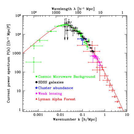
Figure 1: Observational power spectrum from CMB fluctuations, galaxy clustering, gravitational lensing shear, cluster abundances and Lyman $\alpha$ clouds, compared with the prediction of $\Lambda$CDM model. The figure is taken from the SDSS paper, Tegmark et al. [15]

Another important measure is the power spectrum that characterises matter fluctuations,

$$P(k)=\int d^{3}xe^{ik\cdot x}\langle\delta(x)\delta(0)\rangle,$$ (6)

where $\delta(x)$ is the density contrast at the position $x$. A variety of observations at vastly different cosmological epochs (CMB at $z=1090$, galaxy clustering at $z\sim 0.1-0.4$, gravitational lensing at $z\sim 0.5-1$, cluster abundances at $z\sim 0.1-0.2$), when scaled to $z=0$, yield $P(k)$ that is described by $|k|^{n}T(k)$ with $n=1\pm 0.02$ and the transfer function $T(k)$ predicted by the $\Lambda$CDM model with the cosmological parameters specified above [15, 16] (see Figure 1). This consistent description of $P(k)$ constitutes additional evidence that supports the standard model, nearly scale-invariant initial adiabatic perturbations ($\delta=3\delta T/T$) growing by gravitational instability in the $\Lambda$CDM universe. We must add a remark that no models are known, other than inflation, that generate these fluctuations consistent with observations, while a successful model of inflation from the particle physics point of view is yet to be found.

The massive neutrinos contribute to the mass density of the Universe by the amount

$$\Omega_{\nu}=\frac{\sum m_{\nu}}{94.1~{}{\rm eV}}h^{-2},$$ (7)

where $h=0.71$ is the conventional notation for the Hubble constant. In the following discussion we assume three species of light neutrinos and do not consider exotic possibilities which are occasionally discussed by particle physicists. The neutrino mass and its limits discussed in what follows are of the order of 1 eV, which is much larger than than 0.05 eV derived for the mass difference for the limiting case of the hierarchical-mass neutrinos. It is therefore appropriate to consider three degenerate neutrinos, and we assume this in our considerations.

3.1 Effects of massive neutrinos on the evolution of cosmic fluctuations

A successful model is obtained for cosmic structure formation without having massive neutrinos. This means that massive neutrinos only disturb the agreement between theory and observations, hence leading to a limit on the neutrino mass.

The well-known effect of massive neutrinos is relativistic free streaming that damps fluctuations within the horizon scale. One electron volt neutrinos are still relativistic at matter-radiation equality, which takes place at $T\approx 1$ eV, and then tend to smear fluctuations up to $\sim$100 Mpc comoving scale, thus diminishing the power of $P(k)$ for these scales. This effect becomes stronger as the cosmological mass density of neutrinos, hence the neutrino mass, increases (see Figure 2) (see [17, 18]). Therefore, the empirical knowledge of $P(k)$ across large to small scales gives a constraint on the summed mass of neutrinos.

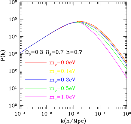
Figure 2: Power spectrum predicted in the $\Lambda$CDM model including massive neutrinos with a degenerate mass specified in the legend. The top curve represents the case of massless neutrinos

The best determination of $P(k)$ for large scales is given by CMB multipoles observed by WMAP [1]. There are a number of ways to obtain $P(k)$ at small scales: the use of galaxy clustering, the cluster abundance, the Lyman $\alpha$ cloud absorption optical depth, and the cosmic shear due to gravitational lensing. Limits on the neutrino mass are derived from a single or combined use of these observations. One may also input other observations, which serve to restrict various cosmological parameters, which may indirectly improve the limit on the neutrino mass in a multidimensional parameter search.

(1) Limits derived from galaxy clustering varies from $\sum m_{\nu}<0.6$ eV [12] to 2.1 eV [19] at a 95% confidence, both authors using 2dFGRS data (see also [20]). The limit using the SDSS data is $\sum m_{\nu}<1.7$ eV [13]. (See also [21], where $\sum m_{\nu}<0.75$ eV is concluded using SDSS and 2dFGRS.) While I quoted the limits all obtained by using only CMB and galaxy clustering here, the origin of different upper limits is not clear. It is possible that the use of SDSS or 2dFGRS would leads to different limits, as the fall of $P(k)$ towards smaller scales is more gentle with the 2dFGRS, thus giving a stronger constraint on $m_{\nu}$. A suspect is the convergence of practical applications of the Markov chain Monte Carlo method to calculate the likelihood, which we discuss briefly in section 3.3.

(2) The use of the cluster abundance enables us to estimate the mass fluctuations that are the quantity relevant to us. This was made in the early work [22], but no updates were attempted after WMAP.

(3) With the Lyman $\alpha$ cloud absorption power derived from fluctuating optical depths, one can explore $P(k)$ at the smallest scale [23, 24], giving the strongest limit $\sum m_{\nu}<0.42$ eV (95%) [25] (see [26] for the earlier work). This result, however, is more model dependent in the sense that one must invoke simulations to extract $P(k)$ from observed flux power spectrum, which suffer from significant uncertainties associated with modelling and simulations.

(4) With gravitational lensing one can directly explore mass fluctuations. For the moment the statistical error is not sufficiently small, but this provides us with a promising method. This may also be used to set the normalisation of the power spectrum derived from galaxy clustering.

Elgarøy and Lahav [27] give a summary of limits obtained in the literature.

We note that a decrease of spectral index $n$ (red tilting) has an effect similar to that of massive neutrinos for small scales. Hence, unless the length scale explored spans a wide range or $n$ is constrained, $m_{\nu}$ and $n$ are positively correlated, i.e., an ‘artificial’ blue tilting would be cancelled by an appropriate value of $m_{\nu}$; this weakens the constraint on $m_{\nu}$. Elgarøy et al. [28] derived from 2dFGRS power spectrum ‘alone’ $\sum m_{\nu}<2$ eV, but this is under the assumption that the spectrum is exactly flat, $n=1$. Allowing for $n>1$, a sensible limit is lost. We definitely need CMB data to derive a limit on the neutrino mass.

3.2 Cosmological limits on the neutrino mass: caveats

The methods listed above all suffer from different systematic errors. What we really need is the mass fluctuation $\xi_{m}=\langle\delta_{m}(x)\delta_{m}(0)\rangle$ in the linear regime. We expect that nonlinearity for the length scale relevant to galaxy clustering $>10$ Mpc is only modest (e.g. [29]), but with the use of galaxy clustering we must assume that the galaxy distribution traces mass allowing for some constant factor, i.e., $\xi_{g}(x)=b^{2}\xi_{m}(x)$, where $b$ is left usually as a free parameter, representing “biasing” of galaxies relative to mass. This is probably not a bad approximation at the accuracy that concerns us at the present, but for higher accuracy we do not know how good is this approximation: at least we know that biasing depends on morphology and luminosity of galaxies (e.g., [30]). Hence the sample used must be homogeneous in this regard. The systematic difference in $P(k)$ between the two groups must also be resolved. It should also be noted that errors for the galaxy clustering data given in the literature may not represent properly the systematics that are associated with the evaluation of the window function of the survey data analysis.

The use of the cluster abundance is proposed as a way to estimate the mass fluctuation taking advantage that the cluster mass can be estimated with various means, from velocity dispersion measurements, X ray data, and gravitational lensing. For the moment, however, there are non-negligible uncertainties in the cluster mass estimate. The disadvantage of this method is that one needs a very large cluster sample to estimate $P(k)$ for varying scales.

One can explore mass fluctuations in the smallest scale with the use of Lyman $\alpha$ cloud absorption power spectrum; thus one can get potentially the information most sensitive to $m_{\nu}$. The problem is that one needs substantial corrections to unfold the matter power spectrum $P(k)$, which can be done only with simulations. While a great success of numerical study was to enable us understand the nature of Lyman $\alpha$ clouds [31] (see [32] for a review), it is not easy at a quantitative level to document the systematic errors. The simulation always suffers from mesh effects, and this is particularly true when baryons are included. With the inclusion of baryons one has to deal with stars and their feedback, which is a difficult astrophysical problem. Specifically for the case of Lyman $\alpha$ clouds, we must be concerned with uncertainties as to the heating rate from ionising radiation and thermal history of clouds. The estimate of the mean level of absorption optical depths is an additional source of errors. While much work is currently being done, the assessment of errors in $P(k)$ derived from Lyman $\alpha$ clouds is not easy a problem.

In principle the use of cosmic shear is the best for estimating the mass fluctuation. The nonlinearity correction is still needed, but it can be done with simulations without baryons, which are relatively simple. A difficulty is that the signal is small compared with noise so that one needs a very large galaxy sample to attain good statistics, and that one needs to know instrumental distortions of images accurately.

3.3 Limits on neutrino mass from CMB alone?

There is a controversy as to whether a sensible limit is derived on the neutrino mass from CMB multipoles alone. This consideration is meaningful since one might be able to derive the most robust limit on the neutrino mass free from systematics that are difficult to control with data on galaxies. Tegmark et al. [13], however, showed that no limits are obtained from CMB alone: $\sum m_{\nu}<9$ eV is allowed at one sigma. Elgarøy & Lahav [33] endorsed this result, emphasising the need to employ large-scale structure data. They also suggest that there is a solution that reproduces CMB multiples only with CDM and massive neutrinos that satisfy $\Omega_{m}+\Omega_{\nu}=1$ without a cosmological constant, i.e., the ‘old’ mixed dark matter (MDM) scenario is viable (see Figure 3), with the only price being a low Hubble constant.

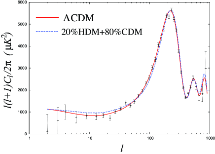
Figure 3: CMB multipoles for the MDM like solution suggested by Elgarøy & Lahav ($\sum m_{\nu}=4$ eV, dotted curve) are compared with those for the best $\Lambda$CDM solution (with massless neutrinos, solid curves). The $\chi^{2}$ is higher by 50 with this MDM like solution. The data are from WMAP.

On the other hand, Ichikawa, Fukugita & Kawasaki [34] claimed that a sensible limit $\sum m_{\nu}<2$ eV (at a 95% confidence) can be derived from CMB (WMAP data) alone. They argued that the effects of massive neutrinos on CMB multipoles cannot be absorbed into the shift of cosmological parameters (notably the Hubble constant) if neutrinos are already nonrelativistic at the recombination epoch, i.e., $m_{\nu}\mathrel{\mathchoice{\lower 3.0pt\vbox{\halign{$\m@th\displaystyle\hfill#\hfil$\cr>\crcr\sim\crcr}}}{\lower 3.0pt\vbox{\halign{$\m@th\textstyle\hfill#\hfil$\cr>\crcr\sim\crcr}}}{\lower 3.0pt\vbox{\halign{$\m@th\scriptstyle\hfill#\hfil$\cr>\crcr\sim\crcr}}}{\lower 3.0pt\vbox{\halign{$\m@th\scriptscriptstyle\hfill#\hfil$\cr>\crcr\sim\crcr}}}}3T_{\rm rec}\simeq 0.55$ eV. The principle is that the presence of non-relativistic neutrinos causes a decay of gravitational potential in pre-recombination epoch, which amplifies the acoustic oscillation that appears as the second and third peaks [35] (while the first peak receives little the effect from the potential decay, since the multipoles corresponding to free streaming of the $m_{\nu}\mathrel{\mathchoice{\lower 3.0pt\vbox{\halign{$\m@th\displaystyle\hfill#\hfil$\cr>\crcr\sim\crcr}}}{\lower 3.0pt\vbox{\halign{$\m@th\textstyle\hfill#\hfil$\cr>\crcr\sim\crcr}}}{\lower 3.0pt\vbox{\halign{$\m@th\scriptstyle\hfill#\hfil$\cr>\crcr\sim\crcr}}}{\lower 3.0pt\vbox{\halign{$\m@th\scriptscriptstyle\hfill#\hfil$\cr>\crcr\sim\crcr}}}}0.55$ eV neutrino are $\ell\mathrel{\mathchoice{\lower 3.0pt\vbox{\halign{$\m@th\displaystyle\hfill#\hfil$\cr>\crcr\sim\crcr}}}{\lower 3.0pt\vbox{\halign{$\m@th\textstyle\hfill#\hfil$\cr>\crcr\sim\crcr}}}{\lower 3.0pt\vbox{\halign{$\m@th\scriptstyle\hfill#\hfil$\cr>\crcr\sim\crcr}}}{\lower 3.0pt\vbox{\halign{$\m@th\scriptscriptstyle\hfill#\hfil$\cr>\crcr\sim\crcr}}}}250$ which are larger than the position of the first peak, $\ell_{1}=220$).

The shifts of the position and the height of the first peak, dominantly caused by modifications of the angular diameter distance and of the integrated Sachs-Wolfe effect, respectively, are still significant for $m_{\nu}<0.55$ eV, but the heights of the second and third peaks relative to the first are hardly modified. These effects can be absorbed into the shift of the other cosmological parameters. When the second and third peaks change in addition for $m_{\nu}>0.55$ eV, however, one cannot absorb the effects into the shift of cosmological parameters. This is the basic mechanism how the constraint on $m_{\nu}$ is derived from CMB multipoles. The Hubble constant prior as claimed in [33] is not essential. The numerical analysis of Ichikawa et al. showed that the increase of $\chi^{2}$ with the neutrino mass is very slow till $\sum m_{\nu}\approx 1.5$ eV and gave $\sum m_{\nu_{i}}<2.0~{}{\rm eV}$ at a 95% C.L.

Figure 4 compares the CMB multipoles for the case of $\sum m_{\nu_{i}}=2.0$ eV with the best model having massless neutrinos that gives the global $\chi^{2}$ minimum. This demonstrates the accuracy of the WMAP data, which has a power to distinguish the two curves. It is argued [34] that one cannot obtain a limit significantly better than $0.55\times 3\simeq 1.6$ eV even if the precision of CMB multipoles is improved.

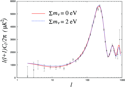
Figure 4: CMB multipoles for the $\Lambda$CDM solution with massive neutrinos that is allowed just at a 95% confidence ($\sum m_{\nu}=2.0$ eV, dashed curve) are compared with those for the best $\Lambda$CDM solution with massless neutrinos (solid curve).The data are from WMAP.

Note that an increase of the peaks at higher $\ell$ modes with massive neutrinos mimics blue tilting, and hence there emerges a negative correlation between $n$ and $m_{\nu}$, which is opposite to that expected from the effect on the power spectrum, as explained in the previous subsection.

Elgarøy & Lahav [27] ascribed the discrepancy between Tegmark et al./ Elgarøy & Lahav and Ichikawa et al. to the difference of priors, but they did not give an analysis that supports this statement. I would ascribe the origin to insufficient samplings of the Markov-chain Monte Carlo methods the former authors adopted to estimate the likelihood functions, especially away from the point at $m_{\nu}=0$. When a chain is not sufficiently long the Markov-chain Monte Carlo methods often result in likelihood functions that differ in shapes depending on the initial condition. This was the reason why Ichikawa et al. preferred to use a deterministic algorithm to search for the minima at given $m_{\nu}$ with successive parabolic approximations, with the further use of the Vegas integration code to check for the likelihood function. In this approach, priors do not play an important role. They also remarked that they could not reproduce the likelihood function of Tegmark et al. as a function of $n$ away from the global minimum, indicating that their likelihood function may probably be incorrectly evaluated, whereas the behaviour around the global minimum was reproduced very well.

Ichikawa et al. further searched for MDM like solutions, but failed to find any with $\Delta\chi^{2}$ smaller than 16. The curves shown in Figure 3 is the solution suggested by Elgarøy & Lahav [33] which gives $\chi^{2}$ higher than the best solution by $\Delta\chi^{2}=50$. Although the shape of the multipoles appears similar to that of the best $\Lambda$CDM solution to eyes, the accuracy of the WMAP data rules out the MDM model at a high confidence.

3.4 Conclusions and prospects

I discussed that there are mainly two effects that lead to constraints on the neutrino mass, damping of the small scale power due to neutrino free streaming, and decay of the gravitational potential in the pre-recombination epoch that amplifies the acoustic oscillation in high multipole modes.

The limit on the neutrino mass from cosmic fluctuations is $\sum m_{\nu_{i}}<2$ eV (95%) from CMB alone, which is subject to systematic errors to the least extent. The assumption is that $\Lambda$CDM model is correct and the power spectrum obeys a power law, allowing for a small departure from the power law to the extent as expected in slow-roll inflation. The limit obtained by combining the galaxy clustering with the CMB data is $\sum m_{\nu_{i}}\mathrel{\mathchoice{\lower 3.0pt\vbox{\halign{$\m@th\displaystyle\hfill#\hfil$\cr<\crcr\sim\crcr}}}{\lower 3.0pt\vbox{\halign{$\m@th\textstyle\hfill#\hfil$\cr<\crcr\sim\crcr}}}{\lower 3.0pt\vbox{\halign{$\m@th\scriptstyle\hfill#\hfil$\cr<\crcr\sim\crcr}}}{\lower 3.0pt\vbox{\halign{$\m@th\scriptscriptstyle\hfill#\hfil$\cr<\crcr\sim\crcr}}}}1-1.7$ eV (95%). Unfortunately, the error arising from the Monte Carlo sampling is not well documented, and an accurate limit is yet to be found for a given set of the clustering data. A systematic error in the power spectrum between two major groups is also yet to be resolved. The current most stringent limit is $\sum m_{\nu_{i}}<0.42$ eV (95%) derived with the use of Lyman $\alpha$ cloud absorption power spectrum by unfolding the matter power spectrum with the aid of simulations of the Lyman $\alpha$ cloud. It is not easy to assess its reliability at the moment.

The accuracy of the CMB multipole data will be greatly increased, especially at the higher multipoles with the launch of Planck [36]. However, a straightforward analysis of its data is unlikely to bring a drastic improvement in the constraint on the neutrino mass. Ichikawa et al. considered that the limit that can be achieved from CMB alone will be $\sum m_{\nu_{i}}<1.2$ eV. Efforts to remove systematic errors are needed for small scale clustering data. Particularly important is to enhance the reliability of simulations in a way convincing to everybody and to document errors involved in the results of simulations.

Clearly, the goal is to give a constraint as small as $\sum m_{\nu_{i}}\approx 0.05$ eV, which is the minimum mass indicated by neutrino oscillation experiments. Kaplinghat et al. [37] proposed to use gravitational lensing signals in CMB polarisation. They forecast that one would get a limit $\sum m_{\nu_{i}}<0.15$ eV with Planck, but need a new project particularly sensitive to CMB polarisation to get to $<0.04$ eV. An accurate simulation is also needed to unfold non-linear effects of mass clustering in small scales. Wang et al. [38] proposed to use large cluster surveys. Their forecast is $\sum m_{\nu_{i}}<0.03$ eV by combining cluster survey using LSST [39] with multipoles from Planck. Here the estimate of cluster mass is crucial, which they hope to perform using simulations of clusters.

References

- [1] C. L. Bennett et al., Astrophys. J. Suppl. 148, 1 (2003).
- [2] D. G. York et al., Astron. J. 120, 159 (2000).
- [3] M. Fukugita and T. Yanagida, Phys. Lett. B174, 45 (1986).
- [4] D. Toussaint, S.B. Treiman, F. Wilczek and A. Zee, Phys. Rev. D19, 1036 (1979).
- [5] S. Weinberg, Phys. Rev. Lett. 42, 850 (1979).
- [6] M. Yoshimura, Phys. Lett. 88B, 294 (1979).
- [7] W. Buchmüller, P. Di Bari and M. Plümacher, Nucl. Phys. B665, 445 (2003).
- [8] G. F. Giudice, A. Notari, A. Riotto and A. Strumia, Nucl. Phys. B685, 89 (2004).
- [9] W. Buchmüller, P. Di Bari and M. Plümacher, Ann. Phys. 315, 303 (2005).
- [10] W. Buchmüller, R. D. Peccei and T. Yanagida, arXiv:hep-ph/0502169
- [11] M. Fukugita and T. Yanagida, Physics of Neutrinos and Application to Astrophyics (Springer, Belin, 2003).
- [12] D.N. Spergel et al., Astrophys. J. Suppl. 148, 175 (2003).
- [13] M. Tegmark et al., Phys. Rev. D69, 103501 (2004).
- [14] D. Eisenstein et al., arXiv:astro-ph/0501171
- [15] M. Tegmark et al., Astrophys. J. 606, 702 (2004).
- [16] S. Cole et al., Mon. Not. Roy. astr. Soc. 362, 505 (2005).
- [17] W. Hu, D. J. Eisenstein and M. Tegmark, Phys. Rev. Lett. 80, 5255 (1998).
- [18] R. Valdarnini, T. Kahniashvili and B. Novosyadlyj, Astron. Astrophys. 336, 11 (1998).
- [19] S. Hannestad, JCAP 5. 004 (2003).
- [20] S.W. Allen, R.W. Schmidt and S.L. Bridle, Mon. Not. Roy. astr. Soc. 346, 593 (2003).
- [21] V. Barger, D. Marfatia and A. Tregre, Phys. Lett. B595, 55 (2004).
- [22] M. Fukugita, G.-C. Liu and N. Sugiyama, Phys. Rev. Lett. 84, 1082 (2000).
- [23] R.A.C. Croft, D.H. Weinberg, N. Katz and L. Hernquist, Astrophys. J. 495, 44 (1998).
- [24] P. McDonald et al., arXiv:astro-ph/0405013
- [25] U. Seljak et al., arXiv:astro-ph/0407372
- [26] R.A.C. Croft, W. Hu and R. Davé, Phys. Rev. Lett. 83, 1092 (1999).
- [27] Ø. Elgarøy and O. Lahav, New J. Phys. 7, 61 (2005).
- [28] Ø. Elgarøy et al., Phys. Rev. Lett. 89, 061301 (2002).
- [29] R. E. Smith et al., Mon. Not. Roy. astr. Soc. 341, 1311 (2003).
- [30] I. Zehavi et al., Astrophys. J. 630, 1 (2005)
- [31] R. Cen, J. Miralda-Escude, J.P. Ostriker and M. Rauch, Astrophys. J. 437, L9 (1994).
- [32] M. Rauch, Ann. Rev. Astr. Astrophys. 36, 267 (1998).
- [33] Ø. Elgarøy and O. Lahav, JCAP 04, 123007 (2004).
- [34] K. Ichikawa, M. Fukugita and M. Kawasaki, Phys. Rev. D71, 043001 (2005).
- [35] S. Dodelson, E. Gates and A. Stebbins, Astrophys. J. 467, 10 (1996).
- [36] J.A. Tauber, in ISO Beyond Point Sources: Studies of Extended Infrared Emission, 1999, Madrid, Spain. ed. by R. J. Laureijs, K. Leech and M. F. Kessler, ESA-SP 455, 2000. p. 185.
- [37] M. Kaplinghat, L. Knox and Y.-S. Song, Phys. Rev. Lett. 91, 241301.
- [38] S. Wang et al., Phys. Rev. Lett. 95, 011302 (2005)
- [39] See, www.lsst.org