Deep inelastic scattering near the endpoint
in soft-collinear effective theory

Abstract

We apply the soft-collinear effective theory (SCET) to deep inelastic scattering near the endpoint region. The forward scattering amplitude, and the structure functions are shown to factorize as a convolution of the Wilson coefficients, the jet functions, the parton distribution functions. The behavior of the parton distribution functions near the endpoint region is considered. It turns out that it evolves with the Altarelli-Parisi kernel even in the endpoint region, and the parton distribution function can be factorized further into a collinear part and the soft Wilson line. The factorized form for the structure functions is obtained by the two-step matching, and the radiative corrections or the evolution for each factorized part can be computed in perturbation theory. We present the radiative corrections of each factorized part to leading order in $\alpha_{s}$, including the zero-bin subtraction for the collinear part.

I Introduction

The soft-collinear effective theory (SCET)Bauer:2000ew ; Bauer:2000yr ; Bauer:2001yt is a useful theoretical tool to treat physical processes with energetic light particles in a systematic way. For an energetic particle moving in the $n^{\mu}$ direction, the momentum can be decomposed into

$$p^{\mu}=\frac{\overline{n}\cdot p}{2}n^{\mu}+p_{\perp}^{\mu}+\frac{n\cdot p}{2}\overline{n}^{\mu}\sim\mathcal{O}(Q)+\mathcal{O}(\Lambda)+\mathcal{O}(\Lambda^{2}/Q),$$ (1)

where $Q$ is a large scale, and $n^{\mu}$, $\overline{n}^{\mu}$ are lightlike vectors satisfying $n^{2}=\overline{n}^{2}=0$, $n\cdot\overline{n}=2$. Each component has a distinct scale in powers of $\Lambda$ which is a typical hadronic scale, and SCET describes the interactions of the collinear particles and the ultrasoft (usoft) particles with momentum $p_{us}^{\mu}\sim(\Lambda,\Lambda,\Lambda)$. Since there are three distinct scales for the momentum of a collinear particle, SCET employs a two-step matching process by integrating out large energy scales successively Bauer:2001yt . In the first stage the degrees of freedom of order $Q$ from the full theory are integrated out to produce $\mathrm{SCET}_{\mathrm{I}}$. In $\mathrm{SCET}_{\mathrm{I}}$, collinear particles are allowed to interact with usoft particles and the typical virtuality of the collinear particles is $p^{2}_{hc}\sim Q\Lambda$. In the second stage the degrees of freedom with $p^{2}\sim Q\Lambda$ are integrated out, and the remaining effective theory in which all the particles have $p^{2}\sim\Lambda^{2}$ is called $\mathrm{SCET}_{\mathrm{II}}$. Here the collinear particles are decoupled from the soft particles. The Wilson coefficients of operators and the renormalization behavior of them can be computed perturbatively by matching the effective theories at each boundary.

SCET has been successfully applied to various $B$ meson decays Chay:2002vy ; Htl ; Leptonic ; Chay:2003ju ; Nonleptonic ; Mantry:2003uz ; Chay:2003kb ; Bauer:2000ew ; Inclusive . It is especially convenient to study the factorization properties of $B$ decays including spectator interactions since SCET is formulated such that soft and collinear particles are decoupled. On the other hand, SCET can be applied to other high-energy processes which include energetic light particles Bauer:2002nz ; Quarkonium ; Chay:2004zn ; Manohar:2003vb ; Jet . It has been applied to deep inelastic scattering (DIS) near the endpoint region using SCET Manohar:2003vb ; Becher:2006mr and using an effective theory scheme Chen:2006vd .

In this paper we analyze the endpoint region in DIS more carefully using the two-step matching to show the explicit factorization of the structure functions in terms of the hard part, the jet function, the soft gluon emissions, and the collinear matrix elements. We also discuss and compare delicate physical meanings and implications of the parton distribution functions in the endpoint region, defined both in the full theory and in SCET. In addition to showing the factorization, we take one step further to consider another aspect of DIS, namely the behavior of the longitudinal structure function near the endpoint region. The longitudinal structure function vanishes at leading order in $\alpha_{s}$ due to the fact that the parton (quark) in the proton has spin 1/2. However this is broken at order $\alpha_{s}$ and the longitudinal structure function is further suppressed by $\Lambda/Q$, which we explicitly present here.

In Section II we explain the kinematics of DIS. We choose the Breit frame and present how the momenta scale in powers of $\Lambda$, which is useful in constructing and matching effective theories. The forward scattering amplitude, and the structure functions are defined in SCET, compared with those in the full theory. In Section III the method to compute the forward scattering amplitudes in DIS using SCET is described. The leading and the subleading currents are introduced and the prescription for the usoft factorization is explained. In Section IV, we compute the structure function $F_{1}(x,Q)$, and show that it factorizes. In Section V, we consider the parton distribution near the endpoint region, and express the forward scattering amplitude in terms of the parton distribution function. In Section VI, we present the moments of the structure functions as a product of the moments for each factorized term. In Section VII, we compute the radiative corrections of each factorized term to order in $\alpha_{s}$, and express the moments of the structure functions to leading logarithmic accuracy. In Section VIII, we compute the longitudinal structure function $F_{L}(x,Q)$ in SCET and show that it also factorizes. In the final section, we give a conclusion. In Appendix A, the zero-bin subtraction method Manohar:2006nz in $\mathrm{SCET}_{\mathrm{I}}$ before the usoft factorization of the collinear fields is discussed. In Appendix B, the procedure for taking the imaginary part in $\mathrm{SCET}_{\mathrm{I}}$ and $\mathrm{SCET}_{\mathrm{II}}$ is explained. In Appendix C, the anomalous dimension of the operator $J_{\mu}^{(1b)}$ is computed to order $\alpha_{s}$.

II Kinematics

Let us consider the electroproduction in DIS $ep\rightarrow eX$ near the endpoint region. The hadronic process consists of $\gamma^{*}p\rightarrow X$, and we choose the Breit frame in which the incoming proton is in the $\overline{n}^{\mu}$ direction, and the outgoing hadrons are mainly in the $n^{\mu}$ direction. The momentum transfer $q^{\mu}$ from the leptonic system is given by

$$q^{\mu}=(\overline{n}\cdot q,q_{\perp}^{\mu},n\cdot q)=(Q,0,-Q)=\frac{Q}{2}(n^{\mu}-\overline{n}^{\mu}),$$ (2)

where $q^{2}=-Q^{2}$ is the large scale. The Bjorken variable $x$ is defined as

$$x=\frac{Q^{2}}{2P\cdot q}\sim\frac{Q}{n\cdot P},$$ (3)

where $P^{\mu}$ is the proton momentum in the $\overline{n}^{\mu}$ direction. The momenta of the proton $P^{\mu}$ and the final-state particles $p_{X}=P+q$ are given by

$$P^{\mu} = (\overline{n}\cdot P,P_{\perp}^{\mu},n\cdot P)\sim\Bigl{(}\frac{x\Lambda^{2}}{Q},P_{\perp}^{\mu},\frac{Q}{x}\Bigr{)},$$

$$p_{X}^{\mu} = (\overline{n}\cdot p_{X},p_{X\perp}^{\mu},n\cdot p_{X})\sim\Bigl{(}Q,p_{X\perp}^{\mu},\frac{1-x}{x}Q\Bigr{)},$$ (4)

with $P^{2}\sim\Lambda^{2}$, $p_{X}^{2}=Q^{2}(1-x)/x$ where $\Lambda$ is a typical hadronic scale of order 1 GeV. Near the endpoint where $x$ approaches 1 ($1-x\sim\Lambda/Q$), the invariant mass squared of the final-state particles becomes $p_{X}^{2}\sim Q^{2}(1-x)\sim Q\Lambda$. Then the final-state particles can be regarded as collinear particles in $\mathrm{SCET}_{\mathrm{I}}$, which are integrated out to obtain $\mathrm{SCET}_{\mathrm{II}}$ through the two-step matching procedure.

At the parton level, let $p^{\mu}$ be the momentum of the incoming parton inside the proton, and let $y$ be the longitudinal momentum fraction ($n\cdot p=yn\cdot P$). Then the partonic Bjorken variable $w$ is given as

$$w=\frac{Q^{2}}{2p\cdot q}\sim-\frac{n\cdot q}{n\cdot p}=\frac{x}{y}.$$ (5)

The momentum of the outgoing parton as $p^{\prime\mu}$ can be written as

$$p^{\prime\mu}=p^{\mu}+q^{\mu}=(\overline{n}\cdot p^{\prime},p_{\perp}^{\prime\mu},n\cdot p^{\prime})\sim(Q,p^{\prime\mu}_{\perp},(1-w)n\cdot p).$$ (6)

And the endpoint region corresponds to $1-w\sim\Lambda/Q$ such that $p^{\prime 2}\sim Q\Lambda$.

The spin-averaged cross section for DIS can be written as

$$d\sigma=\frac{d^{3}{\bf k}^{\prime}}{2|{\bf k}^{\prime}|(2\pi)^{3}}\frac{\pi e^{4}}{sQ^{4}}L^{\mu\nu}(k,k^{\prime})W_{\mu\nu}(p,q),$$ (7)

where $k$ and $k^{\prime}$ are the incoming and outgoing lepton momenta with $q=k^{\prime}-k$, $L^{\mu\nu}$ is the lepton tensor, and $s=(p+k)^{2}$. The hadronic tensor $W_{\mu\nu}$ is related to the imaginary part of the forward scattering amplitude $T^{\mu\nu}$. The forward scattering amplitude is the spin-averaged matrix element of the time-ordered product of the electromagnetic currents, written as

$$T_{\mu\nu}(x,Q)=\langle P|\hat{T}_{\mu\nu}|P\rangle_{\mathrm{spin\ av.}},\ \ \hat{T}_{\mu\nu}(x,Q)=i\int d^{4}ze^{iq\cdot z}T\Bigl{[}J_{\mu}^{\dagger}(z)J_{\nu}(0)\Bigr{]},$$ (8)

where $J_{\mu}$ is the electromagnetic current. The relation between the hadronic tensor $W_{\mu\nu}$ and the forward scattering amplitude $T_{\mu\nu}$ is given by

$$W_{\mu\nu}(x,Q)=\frac{1}{\pi}\mathrm{Im}\,T_{\mu\nu}(x,Q).$$ (9)

In electroproduction, considering all the possible Lorentz structure, $T_{\mu\nu}$ can be generally written as

$$T_{\mu\nu}(x,Q)=-g^{\perp}_{\mu\nu}T_{1}+(\overline{n}_{\mu}n_{\nu}+\overline{n}_{\nu}n_{\mu})T_{2}+(\overline{n}_{\mu}n_{\nu}-\overline{n}_{\nu}n_{\mu})T_{3}+\overline{n}_{\mu}\overline{n}_{\nu}T_{4}+n_{\mu}n_{\nu}T_{5},$$ (10)

where $g^{\perp}_{\mu\nu}=g_{\mu\nu}-(n_{\mu}\overline{n}_{\nu}+\overline{n}_{\mu}n_{\nu})/2$. Due to the current conservation ($q_{\mu}T^{\mu\nu}=0)$, and the parity conservation, we have $T_{4}=T_{5}=T_{2}$, and $T_{3}=0$. Therefore the forward scattering amplitude has two independent quantities, and is given by

$$T_{\mu\nu}(x,Q)=-g^{\perp}_{\mu\nu}T_{1}(x,Q)+(n_{\mu}+\overline{n}_{\mu})(n_{\nu}+\overline{n}_{\nu})T_{2}(x,Q).$$ (11)

This can be cast into different forms using the fact that and any terms proportional to $q_{\mu}=Q(n_{\mu}-\overline{n}_{\mu})/2$ can be discarded since they vanish when they are contracted with the lepton tensor. We can write $n_{\mu}+\overline{n}_{\mu}=(\overline{n}_{\mu}-n_{\mu})+2n_{\mu}=(n_{\mu}-\overline{n}_{\mu})+2\overline{n}_{\mu}$ and drop the terms proportional to $n_{\mu}-\overline{n}_{\mu}$. Then Eq. (11) can be equivalently written as

$$T_{\mu\nu}(x,Q)=-g^{\perp}_{\mu\nu}T_{1}(x,Q)+4n_{\mu}n_{\nu}T_{2}(x,Q)=-g^{\perp}_{\mu\nu}T_{1}(x,Q)+4\overline{n}_{\mu}\overline{n}_{\nu}T_{2}(x,Q).$$ (12)

The structure functions are defined from the hadronic tensor $W_{\mu\nu}$ as

$$W_{\mu\nu}(x,Q)=-g_{\mu\nu}F_{1}(x,Q)+\frac{P_{\mu}P_{\nu}}{P\cdot q}F_{2}(x,Q),$$ (13)

where the terms proportional to $q_{\mu}$ or $q_{\nu}$ are dropped. Using $P_{\mu}=n\cdot P\overline{n}_{\mu}/2$, $2P\cdot q=n\cdot P\overline{n}\cdot q=Q^{2}/x$, we can write Eq. (13) as

$$W_{\mu\nu}(x,Q) = -g_{\mu\nu}F_{1}(x,Q)+\frac{\overline{n}_{\mu}\overline{n}_{\nu}}{2x}F_{2}(x,Q)$$ (14)

$$= -g^{\perp}_{\mu\nu}F_{1}(x,Q)-\frac{1}{2}(n_{\mu}\overline{n}_{\nu}+\overline{n}_{\mu}n_{\nu})F_{1}(x,Q)+\frac{\overline{n}_{\mu}\overline{n}_{\nu}}{2x}F_{2}(x,Q)$$

$$\longrightarrow -g^{\perp}_{\mu\nu}F_{1}(x,Q)+\frac{\overline{n}_{\mu}\overline{n}_{\nu}}{2}\Bigl{(}\frac{1}{x}F_{2}(x,Q)-2F_{1}(x,Q)\Bigr{)}$$

$$= -g^{\perp}_{\mu\nu}F_{1}(x,Q)+\frac{\overline{n}_{\mu}\overline{n}_{\nu}}{2}F_{L}(x,Q),$$

where we extract $n_{\mu}-\overline{n}_{\mu}$ and discard it to obtain the third relation, and the longitudinal structure function $F_{L}(x,Q)$ is defined as

$$F_{L}(x,Q)=\frac{1}{x}F_{2}(x,Q)-2F_{1}(x,Q).$$ (15)

The Lorentz structure $\overline{n}_{\mu}\overline{n}_{\nu}$ in the final expression of Eq. (14) can be replaced by $n_{\mu}n_{\nu}$. Comparing Eqs. (11) and (14), we obtain the relations

$$F_{1}(x,Q)=\frac{1}{\pi}\mathrm{Im}T_{1}(x,Q),\ F_{L}(x,Q)=\frac{8}{\pi}\mathrm{Im}T_{2}(x,Q).$$ (16)

As we will show explicitly, $T_{1}(x,Q)$ receives the contribution at leading order, and $T_{2}(x,Q)$ is suppressed by $\Lambda/Q$ and $\alpha_{s}$ compared to $T_{1}(x,Q)$. Therefore the Callan-Gross relation $F_{L}=0$ holds to leading order, but is violated at subleading order. Here we also present $F_{L}$ computed using SCET. In fact, the equivalence between Eq. (11) and Eq. (12) turns out to imply nontrivial relations because the subleading contributions proportional to $n^{\mu}n^{\nu}$ and $\overline{n}^{\mu}\overline{n}^{\mu}$ come from different subleading current operators in SCET. The statement that all the expressions are equivalent means that the longitudinal structure functions can be obtained using any subleading current operators and it holds to all orders in $\alpha_{s}$. The nontrivial relation will be verified in this paper at order $\alpha_{s}$.

III Operators in SCET near the endpoint region

In computing the forward scattering amplitude, we first express the electromagnetic current $J_{\mu}$ in terms of the effective fields in $\mathrm{SCET}_{\mathrm{I}}$. The electromagnetic current operator at leading order in SCET is given by

$$\overline{q}\gamma_{\mu}q\rightarrow C(Q,\mu)(J_{\mu}^{(0)}+J_{\mu}^{(0)\dagger})=C(Q,\mu)\Bigl{[}\overline{\xi}_{n}W_{n}\gamma_{\mu}^{\perp}W_{\overline{n}}^{\dagger}~{}\xi_{\overline{n}}+\overline{\xi}_{\bar{n}}W_{\bar{n}}\gamma_{\mu}^{\perp}W_{n}^{\dagger}\xi_{n}\Bigr{]},$$ (17)

where $\xi_{n}$ ($\xi_{\bar{n}}$) is the $n$ ($\overline{n}$) collinear fermion field in SCET. Here $W_{n}$ and $W_{\bar{n}}$ are the collinear Wilson lines

$$W_{n}(x)=\Bigl{[}\sum_{\rm{perms}}\exp\Bigl{(}-g\frac{1}{\overline{n}\cdot\mathcal{P}}\overline{n}\cdot A_{n}(x)\Bigr{)}\Bigr{]},\ W_{\bar{n}}(x)=\Bigl{[}\sum_{\rm{perms}}\exp\Bigl{(}-g\frac{1}{n\cdot\mathcal{P}}n\cdot A_{\bar{n}}(x)\Bigr{)}\Bigr{]}.$$ (18)

Here $A_{n}^{\mu}$ ($A_{\bar{n}}^{\mu}$) is the collinear gluon in the $n^{\mu}$ ($\overline{n}^{\mu}$) direction and the summation over the label momenta is suppressed. The Wilson coefficient $C(Q,\mu)$ is actually an operator and Eq. (17) is written as

$$\overline{\xi}_{n}W_{n}\gamma_{\mu}^{\perp}C(\overline{n}\cdot\mathcal{P}^{\dagger},n\cdot\mathcal{P})W_{\overline{n}}^{\dagger}~{}\xi_{\overline{n}}+\mathrm{h.c.}$$

$$=\int d\omega d\bar{\omega}C(\omega,\bar{\omega})\overline{\xi}_{n}W_{n}\delta(\bar{\omega}-\overline{n}\cdot\mathcal{P}^{\dagger})\gamma_{\mu}^{\perp}\delta(\omega-n\cdot\mathcal{P})W_{\overline{n}}^{\dagger}~{}\xi_{\overline{n}}+\mathrm{h.c.},$$ (19)

where $n\cdot\mathcal{P}$ ($\overline{n}\cdot\mathcal{P}^{\dagger}$) is the operator extracting the label momentum in the $\overline{n}$ ($n$) direction. The operator form in Eq. (III) is useful in deriving the Feynman rules to compute radiative corrections. The hard coefficient $C(Q,\mu)$ can be obtained from matching the full theory onto $\mathrm{SCET}_{\mathrm{I}}$, it is given to order $\alpha_{s}$ as Manohar:2003vb

$$C(Q,\mu)=1+\frac{\alpha_{s}C_{F}}{4\pi}\Bigl{(}-\ln^{2}\frac{Q^{2}}{\mu^{2}}+3\ln\frac{Q^{2}}{\mu^{2}}-8+\frac{\pi^{2}}{6}\Bigr{)}.$$ (20)

The hard coefficient $C(Q,\mu)$ satisfies the renormalization group equation

$$\mu\frac{dC(Q,\mu)}{d\mu}=\gamma_{H}(\mu)C(Q,\mu),\ \ \gamma_{H}(\mu)=\frac{\alpha_{s}(\mu)C_{F}}{2\pi}\Bigl{(}4\ln\frac{\mu}{Q}+3\Bigr{)}.$$ (21)

We can obtain subleading current operators at order $\sqrt{\Lambda/Q}$, which contain either $iD_{n}^{\perp}$ or $iD_{\bar{n}}^{\perp}$. There are two independent operators involving $iD_{n}^{\perp}$, one of which arises from the subleading correction to the fermion field $\xi_{\bar{n}}$

$$\overline{q}\gamma_{\mu}q\rightarrow\overline{\xi}_{n}W_{n}\Bigl{(}1+\frac{\hbox{$/$}\kern-5.0pt\hbox{$\overline{n}$}}{2}W_{n}^{\dagger}i\overleftarrow{\hbox{\large$/$}\kern-7.27847pt\hbox{$D$}_{n}^{\perp}}W_{n}\frac{1}{\overline{n}\cdot\mathcal{P}^{\dagger}}+\cdots\Bigr{)}\gamma_{\mu}W_{\bar{n}}^{\dagger}\xi_{\bar{n}}.$$ (22)

The second term in Eq. (22) yields the subleading current at tree level

$$J_{\mu}^{(1a)}=\overline{\xi}_{n}\frac{\hbox{$/$}\kern-5.0pt\hbox{$\overline{n}$}}{2}i\overleftarrow{\hbox{\large$/$}\kern-7.27847pt\hbox{$D$}_{n}^{\perp}}W_{n}\frac{1}{\overline{n}\cdot\mathcal{P}^{\dagger}}\gamma_{\mu}W_{\bar{n}}^{\dagger}\xi_{\bar{n}}=-\overline{n}_{\mu}\overline{\xi}_{n}i\overleftarrow{\hbox{\large$/$}\kern-7.27847pt\hbox{$D$}_{n}^{\perp}}W_{n}\frac{1}{\overline{n}\cdot\mathcal{P}^{\dagger}}W_{\bar{n}}^{\dagger}\xi_{\bar{n}}.$$ (23)

The second type arises from integrating out the off-shell modes when the collinear quark $\xi_{\bar{n}}$ emits a collinear gluon $A_{n}^{\mu}$, and it is given at tree level as

$$J_{\mu}^{(1b)}=\overline{\xi}_{n}\gamma_{\mu}i\hbox{\large$/$}\kern-7.27847pt\hbox{$D$}_{n}^{\perp}W_{n}\frac{\hbox{$/$}\kern-5.50117pt\hbox{$n$}}{2}\frac{1}{n\cdot\mathcal{P}}W_{\bar{n}}^{\dagger}\xi_{\bar{n}}=-n_{\mu}\overline{\xi}_{n}i\hbox{\large$/$}\kern-7.27847pt\hbox{$D$}_{n}^{\perp}W_{n}\frac{1}{n\cdot\mathcal{P}}W_{\bar{n}}^{\dagger}\xi_{\bar{n}}.$$ (24)

This can be derived by computing the Feynman diagram for the process and by integrating out the intermediate state with virtuality $p^{2}\sim Q^{2}$. And the result can be made gauge invariant by inserting the appropriate collinear Wilson lines. A novel method to derive the operator is the auxiliary field method Bauer:2001yt ; Bauer:2002nz ; Chay:2003ju .

There are other subleading current operators involving $iD_{\bar{n}}^{\perp}$, which can be obtained by expanding $\xi_{\bar{n}}$ to subleading order and by considering the process in which $\xi_{n}$ emits $A_{\bar{n}}^{\mu}$. However these subleading operators do not contribute to the jet function which is obtained by integrating out the degrees of freedom of order $p^{2}\sim Q\Lambda$ in going down to $\mathrm{SCET}_{\mathrm{II}}$ because these subleading operators describe the interaction of the $\overline{n}$-collinear particles in the proton. These operators contribute to the subleading corrections for the parton distribution functions which are given by the matrix elements of the collinear operators in the $\overline{n}^{\mu}$ direction, and we will not consider them here.

Before going down to $\mathrm{SCET}_{\mathrm{II}}$, it is convenient to factor out the usoft interactions by redefining the collinear fields, for example, as

$$\xi_{n}\rightarrow Y_{n}\xi_{n},\ A_{n}^{\mu}\rightarrow Y_{n}A_{n}^{\mu}Y_{n}^{\dagger},\ \ \xi_{\bar{n}}\rightarrow Y_{\bar{n}}\xi_{\bar{n}},\ A_{\bar{n}}^{\mu}\rightarrow Y_{\bar{n}}A_{\bar{n}}^{\mu}Y_{\bar{n}}^{\dagger},$$ (25)

for the collinear fields moving from $-\infty$ to $x$. Once the usoft interactions are factored out, collinear particles do not interact with usoft particles any more. The prescription of the usoft Wilson lines depends on the propagation of the collinear particles or antiparticles to which the soft gluons are attached, and it is described in detail in Ref. Chay:2004zn . The possible usoft Wilson lines are given by

$$Y_{n} = \sum_{\rm{perm}}\exp\Biggl{[}\frac{1}{n\cdot\mathcal{R}+i\epsilon}(-gn\cdot A_{us})\Biggr{]},~{}~{}~{}~{}Y_{n}(x)=P\exp\Biggl{[}ig\int^{x}_{-\infty}ds~{}n\cdot A_{us}\Biggr{]},$$

$$\tilde{Y}_{n} = \sum_{\rm{perm}}\exp\Biggl{[}\frac{1}{n\cdot\mathcal{R}-i\epsilon}(-gn\cdot A_{us})\Biggr{]},~{}~{}~{}~{}\tilde{Y}_{n}(x)=\overline{P}\exp\Biggl{[}ig\int^{\infty}_{x}ds~{}n\cdot A_{us}\Biggr{]},$$ (26)

where $\mathcal{R}$ is the momentum operator for the usoft fields and the path ordering $P$ means that the fields are ordered such that the gauge fields closer (farther) to the point $x$ are moved to the left, while $\overline{P}$ denotes the anti-path ordering. As explained in Ref. Chay:2004zn , $Y_{n}$ ($Y_{n}^{\dagger}$) is the usoft Wilson line attached to the collinear particle (antiparticle) from $-\infty$, while $\tilde{Y}_{n}$ ($\tilde{Y}_{n}^{\dagger}$) is the usoft line attached to the collinear antiparticle (particle) moving to $\infty$. This delicate procedure of choosing the appropriate usoft Wilson lines is related to the $i\epsilon$ prescription, which specifies the location of the poles. Physically, this is related to choosing the sign of $\overline{n}\cdot p$ since the denominator in Eq. (III) is actually $n\cdot\mathcal{R}+i\mathrm{sgn.}(\overline{n}\cdot p)\epsilon$, and the sign of $\overline{n}\cdot p$ depends on whether the collinear field is a particle or an antiparticle.

Now that the current operators at leading and subleading order in SCET are known, we can compute the forward scattering amplitude $T_{\mu\nu}$, or the hadronic tensor $W_{\mu\nu}$ and factorize the usoft interactions using the appropriate prescription for the usoft Wilson lines. Then we integrate out the degrees of freedom of order $p^{2}\sim Q\Lambda$ to obtain the result in $\mathrm{SCET}_{\mathrm{II}}$. In $\mathrm{SCET}_{\mathrm{II}}$ the soft interactions are decoupled from the collinear particles with $p^{2}\sim\Lambda^{2}$, and the decoupled soft particles contribute to the soft Wilson lines which are responsible for the emission of soft gluons.

IV Factorization of $F_{1}(x,Q)$

In $\mathrm{SCET}_{\mathrm{I}}$ after the usoft factorization, the time-ordered product $\hat{T}_{\mu\nu}^{(0)}$ at leading order is written as

$$\hat{T}^{(0)}_{\mu\nu} = iC^{2}(Q)\int d^{4}ze^{i(q+\tilde{p}-\tilde{p}^{\prime})\cdot z}T\Bigl{[}J_{\mu}^{(0)\dagger}(z)J_{\nu}^{(0)}(0)\Bigr{]}$$ (27)

$$= iC^{2}(Q)\int d^{4}ze^{i(q+\tilde{p}-\tilde{p}^{\prime})\cdot z}T\Bigl{[}\overline{\xi}_{\bar{n}}W_{\bar{n}}\tilde{Y}^{\dagger}_{\bar{n}}\gamma_{\mu}Y_{n}W_{n}^{\dagger}\xi_{n}(z)\overline{\xi}_{n}W_{n}Y_{n}^{\dagger}\gamma_{\nu}Y_{\bar{n}}W_{\bar{n}}^{\dagger}\xi_{\bar{n}}(0)\Bigr{]},$$

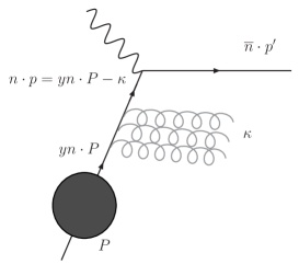
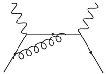
where $\tilde{p}^{\mu}$ and $\tilde{p}^{\prime\mu}$ are the label momenta. Note that $\overline{n}\cdot q=\overline{n}\cdot\tilde{p}^{\prime}$ which ensures the conservation of the label momenta in the $n^{\mu}$ direction, while there is a slight mismatch in the $\overline{n}^{\mu}$ direction near the endpoint $w\sim 1$ such that $n\cdot q+n\cdot\tilde{p}=(1-w)n\cdot p$, which survives in the exponent. The Feynman diagram of the forward scattering amplitude for $\hat{T}_{\mu\nu}^{(0)}$ is sketched in Fig. 1 (a).

Figure 1: (a) Feynman diagram for the forward scattering amplitude in DIS in $\rm{SCET_{I}}$ and (b) the prescription of the (u)soft Wilson lines.

The prescription for the usoft Wilson lines in DIS is described in Fig. 1 (b). It is determined by the external states, which consist of an incoming particle $\xi_{\bar{n}}$ from $-\infty$ to 0, and an outgoing particle $\overline{\xi}_{\bar{n}}$ from $z$ to $\infty$. The intermediate states can move either from 0 to $-\infty$ and then from $-\infty$ to $z$, or from 0 to $\infty$ and then from $\infty$ to $z$. In both cases, the usoft Wilson line survives between 0 and $z$, and the remaining part cancels. Either choice of the intermediate states is appropriate for describing DIS and here we choose the usoft Wilson lines for each current as

$$\overline{\xi}_{n}W_{n}\gamma_{\mu}W_{\bar{n}}^{\dagger}\xi_{\bar{n}}:\ \overline{\xi}_{n}\rightarrow\overline{\xi}_{n}Y_{n}^{\dagger},\ A_{n}^{\mu}\rightarrow Y_{n}A_{n}^{\mu}Y_{n}^{\dagger},\ \xi_{\bar{n}}\rightarrow Y_{\bar{n}}\xi_{\bar{n}},\ A_{\bar{n}}^{\mu}\rightarrow Y_{\bar{n}}A_{\bar{n}}^{\mu}Y_{\bar{n}}^{\dagger},$$

$$\overline{\xi}_{\bar{n}}W_{\bar{n}}\gamma_{\mu}W_{n}^{\dagger}\xi_{n}:\ \overline{\xi}_{\bar{n}}\rightarrow\overline{\xi}_{\bar{n}}\tilde{Y}_{\bar{n}}^{\dagger},\ A_{\bar{n}}^{\mu}\rightarrow\tilde{Y}_{\bar{n}}A_{\bar{n}}^{\mu}\tilde{Y}_{\bar{n}}^{\dagger},\ \xi_{n}\rightarrow Y_{n}\xi,\ A_{n}^{\mu}\rightarrow Y_{n}A_{n}^{\mu}Y_{n}^{\dagger},$$ (28)

where the intermediate state is going from 0 to $-\infty$, then moving from $-\infty$ to $z$. This prescription is used in Eq. (27).

Since there are no collinear particles in the $\overline{n}^{\mu}$ direction in the final state, we obtain the jet function defined by

$$\langle 0|T[W^{\dagger}_{n}\xi_{n}(z)\overline{\xi}_{n}W_{n}(0)]|0\rangle=i\frac{\hbox{$/$}\kern-5.50117pt\hbox{$n$}}{2}\int\frac{d^{4}k}{(2\pi)^{4}}e^{-ik\cdot z}J_{P}(k),$$ (29)

where $P$ is the label momentum and $J_{P}(k)$ depends only on $n\cdot k$. We can simplify $\hat{T}_{\mu\nu}^{(0)}$ using the fact that

$$\int d^{4}z\int\frac{d^{4}k}{(2\pi)^{4}}e^{-ik_{\perp}\cdot z_{\perp}-i\bar{n}\cdot kn\cdot z/2}=\int d^{4}z\frac{1}{4\pi}\int dn\cdot k\delta^{2}(z_{\perp})\delta\Bigl{(}\frac{n\cdot z}{2}\Bigr{)}=\frac{1}{4\pi}\int dn\cdot kd\overline{n}\cdot z,$$ (30)

and plugging the jet function into Eq. (27), we have

$$\hat{T}_{\mu\nu}^{(0)} = -C^{2}(Q)\int d\omega\int\frac{d\overline{n}\cdot zdn\cdot k}{4\pi}e^{i[\omega/2+n\cdot q-n\cdot k]\bar{n}\cdot z/2}J_{P}(n\cdot k)$$ (31)

$$\times T\Bigl{[}\overline{\xi}_{\bar{n}}W_{\bar{n}}\tilde{Y}_{\bar{n}}^{\dagger}Y_{n}\Bigl{(}\frac{\overline{n}\cdot z}{2}\Bigr{)}\delta(\omega-\mathcal{P}_{+})\gamma_{\mu}\frac{\hbox{$/$}\kern-5.50117pt\hbox{$n$}}{2}\gamma_{\nu}Y_{n}^{\dagger}Y_{\bar{n}}W_{\bar{n}}^{\dagger}\xi_{\bar{n}}(0)\Bigr{]}$$

$$= -C^{2}(Q)\int d\omega\int\frac{d\overline{n}\cdot zdn\cdot k}{4\pi}\int d\eta e^{i[\omega/2+n\cdot q-n\cdot k-\eta]\bar{n}\cdot z/2}J_{P}(n\cdot k)$$

$$\times T\Bigl{[}\overline{\xi}_{\bar{n}}W_{\bar{n}}\delta(\omega-\mathcal{P}_{+})\gamma^{\mu}\frac{\hbox{$/$}\kern-5.50117pt\hbox{$n$}}{2}\gamma_{\nu}\tilde{Y}_{\bar{n}}^{\dagger}Y_{n}\delta(\eta+n\cdot i\partial)Y_{n}^{\dagger}Y_{\bar{n}}W_{\bar{n}}^{\dagger}\xi_{\bar{n}}(0)\Bigr{]}$$

$$\longrightarrow -~{}C^{2}(Q)\int d\omega\int dn\cdot k\int d\eta\delta\Bigl{(}\frac{\omega}{2}+n\cdot q-n\cdot k-\eta\Bigr{)}J_{P}(n\cdot k)$$

$$\times \frac{1}{N}\langle 0|\mathrm{tr}\Bigl{[}\tilde{S}_{\bar{n}}^{\dagger}S_{n}\delta(\eta+n\cdot i\partial)S_{n}^{\dagger}S_{\bar{n}}\Bigr{]}|0\rangle~{}\overline{\xi}_{\bar{n}}W_{\bar{n}}\delta(\omega-\mathcal{P}_{+})\gamma_{\mu}\frac{\hbox{$/$}\kern-5.50117pt\hbox{$n$}}{2}\gamma_{\nu}W_{\bar{n}}^{\dagger}\xi_{\bar{n}}(0)$$

$$= -C^{2}(Q)\int d\omega\int d\eta J_{P}\Bigl{(}\frac{\omega}{2}+n\cdot q-\eta\Bigr{)}S(\eta)\overline{\xi}_{\bar{n}}W_{\bar{n}}\delta(\omega-\mathcal{P}_{+})\gamma_{\mu}\frac{\hbox{$/$}\kern-5.50117pt\hbox{$n$}}{2}\gamma_{\nu}W_{\bar{n}}^{\dagger}\xi_{\bar{n}},$$

where the usoft Wilson line $Y_{n}$ ($Y_{\bar{n}}$) in $\mathrm{SCET}_{\mathrm{I}}$ is replaced by the soft Wilson line $S_{n}$ ($S_{\bar{n}}$) in $\mathrm{SCET}_{\mathrm{II}}$. Here the operator $\mathcal{P}_{+}=n\cdot\mathcal{P}+n\cdot\mathcal{P}^{\dagger}$ is the sum of the label momenta. Since the soft interaction is decoupled from the collinear sector, the soft Wilson lines are pulled out, and are described by the vacuum expectation of the soft Wilson line $S(\eta)$, which is given by

$$S(\eta)=\frac{1}{N}\langle 0|\mathrm{tr}\Bigl{[}\tilde{S}_{\bar{n}}^{\dagger}S_{n}\delta(\eta+n\cdot i\partial)S_{n}^{\dagger}S_{\bar{n}}\Bigr{]}|0\rangle.$$ (32)

The delta function in Eq. (31) states that the momentum conservation in the $n$ direction includes the soft momentum from soft gluons. Eq. (31) is the factorized form for the leading forward scattering amplitude. It consists of the hard part $C^{2}(Q)$, obtained in matching the current between the full theory and $\mathrm{SCET}_{\mathrm{I}}$, the jet function $J_{P}(n\cdot k)$, obtained in matching between $\mathrm{SCET}_{\mathrm{I}}$ and $\mathrm{SCET}_{\mathrm{II}}$, and the remaining collinear and soft operators in $\mathrm{SCET}_{\mathrm{II}}$, whose matrix elements are given by nonperturbative parameters. The radiative corrections or the renormalization group evolution of each term can be computed in perturbation theory.

Note that the final operators in $\mathrm{SCET}_{\mathrm{II}}$ show a peculiar structure. In inclusive $B$ decays, the final operator after the two-step matching is a heavy quark bilinear operator with the soft Wilson lines. The matrix element of this operator is parameterized by the shape function of the $B$ meson Bauer:2003pi . This is because the final operator is made of soft particles. But in DIS, the final operators are made of the collinear operators and the soft Wilson line. The soft Wilson line is responsible for the soft gluon emission and the parton distribution function near the endpoint is affected by this when a collinear particle participates in the hard scattering. It is a general feature for physical processes with collinear external particles that the soft Wilson line does not completely cancel near the endpoint, and it describes the soft gluon emission in the process.

V parton distribution function

We can extract $T_{1}^{(0)}$, proportional to $-g_{\mu\nu}^{\perp}$ in $\hat{T}_{\mu\nu}^{(0)}$ from Eq. (31), and it is given by

$$T_{1}^{(0)} = -C^{2}(Q)\int d\omega\int\frac{dzdn\cdot k}{2\pi}\int d\eta e^{i[\omega/2+n\cdot q-n\cdot k-\eta]z}J_{P}(n\cdot k)S(\eta)$$ (33)

$$\times \langle P|\overline{\xi}_{\bar{n}}W_{\bar{n}}\delta(\omega-\mathcal{P}_{+})\frac{\hbox{$/$}\kern-5.50117pt\hbox{$n$}}{2}W_{\bar{n}}^{\dagger}\xi_{\bar{n}}(0)|P\rangle_{\mathrm{spin\ av.}},$$

where $z=\overline{n}\cdot z/2$. We want to express Eq. (33) in terms of the parton distribution functions. Here we consider only the flavor nonsinglet contribution. The standard coordinate space definitions Soper:1996sn for the proton parton distribution functions $f_{P}^{q}(y)$ for quarks of flavor $q$ moving in the $\overline{n}$ direction in full QCD are given as

$$f_{P}^{q}(y)=\int\frac{dz}{2\pi}e^{-iyzn\cdot P}\langle P(P)|\overline{q}(z)Y(z,0)\frac{\hbox{$/$}\kern-5.50117pt\hbox{$n$}}{2}q(0)|P(P)\rangle_{\mathrm{spin\ av.}},$$ (34)

where $Y(y,0)$ is the path-ordered Wilson line and $|P(P)\rangle$ is the proton state with momentum $P^{\mu}$. Here $y$ is defined as the longitudinal momentum fraction of the parton before the hard scattering and that of the proton, $n\cdot p=yn\cdot P$.

Figure 2: An energetic parton comes out of the proton with the momentum $yn\cdot P$. It emits soft gluons with momentum $\kappa$, and the momentum of the hard parton before the hard scattering becomes $yn\cdot P-\kappa$.

The definition of the parton distribution function in Eq. (34) is appropriate away from the endpoint region. But near the endpoint region, we have to extend the definition of the parton distribution to include the effect of the soft gluon emission, satisfying the requirement that it approach Eq. (34) away from the endpoint region. At first sight, the soft momentum does not affect the parton distribution function since it describes the large energy component of the parton. In order to see why this is not so, let us consider a parton near the endpoint region undergoing a hard collision, as depicted in Fig. 2. First a parton with the longitudinal momentum fraction $y$ comes out of the proton. It emits soft gluons with total momentum $\kappa\sim\Lambda_{\mathrm{QCD}}$ before it undergoes a hard collision with a photon. The parton distribution function $f_{P}^{q}(n\cdot p/n\cdot P)$ describes the probability of a parton entering the hard collision with the longitudinal momentum fraction $n\cdot p=yn\cdot P-\kappa$. When $yn\cdot P\gg\Lambda_{\mathrm{QCD}}$ including the endpoint region, the inclusion of $\kappa$ seems to give a negligible effect. When we take a time-ordered product of this current as in Fig. 1 (a), all the soft gluons are attached to the $n$-collinear outgoing fermion due to the property of the soft interactions, which means that all the soft gluons are real gluons when we take the discontinuity. Away from the endpoint region, $n\cdot p^{\prime}$ and $\overline{n}\cdot p^{\prime}$ of the $n$-collinear quark are of order $Q$, and are not affected by the interaction of the soft gluons, that is, $n\cdot p^{\prime}$ does not change to leading order in $\Lambda$. Therefore the interaction of the soft gluons can be neglected and we can safely put $\kappa=0$.

Near the endpoint region, however, $n\cdot p^{\prime}$ is of order $\Lambda$ and the interaction with the soft gluons can significantly affect $n\cdot p^{\prime}$. If a physical quantity depends on the term proportional to $1/n\cdot p^{\prime}$, like the jet function, we have to keep the momentum $\kappa$ of the soft gluons carefully. From the above argument, the parton distribution function in Eq. (34) can be extended in the endpoint region as

$$f_{P}^{q}(y,\kappa)=\int\frac{dz}{2\pi}e^{-iz(yn\cdot P-\kappa)}\langle P(P)|\overline{q}(z)Y(z,0)\frac{\hbox{$/$}\kern-5.50117pt\hbox{$n$}}{2}q(0)|P(P)\rangle_{\mathrm{spin\ av.}},$$ (35)

where the naive $yn\cdot P$ is replaced by $yn\cdot P-\kappa$, that is, the parton distribution function is a function of the large longitudinal momentum fraction $y$, and the momentum of the soft gluons $\kappa$. The Wilson line $Y(z,0)$ in Eq. (34) is the Wilson line with the gauge field in full QCD. However, by looking at the kinematics near the endpoint, the Wilson line can be decomposed into the collinear and the soft Wilson lines Korchemsky:1992xv . This procedure is similar to the approach in SCET, and SCET makes this procedure manifest.

The parton distribution function in $\mathrm{SCET}_{\mathrm{II}}$ can be written as

$$f_{P}^{q}(y,\kappa) = \int d\omega\int\frac{dz}{2\pi}e^{i(\omega/2-yn\cdot P+\kappa)z}\langle P_{\bar{n}}|\Bigl{[}\overline{\xi}_{\bar{n}}W_{\bar{n}}\Bigr{]}\tilde{S}_{\bar{n}}^{\dagger}S_{n}(z)\frac{\hbox{$/$}\kern-5.50117pt\hbox{$n$}}{2}\delta(\omega-\mathcal{P}_{+})S_{n}^{\dagger}S_{\bar{n}}\Bigl{[}W_{\bar{n}}^{\dagger}\xi_{\bar{n}}\Bigr{]}(0)|P_{\bar{n}}\rangle$$ (36)

$$= \int d\omega\int\frac{dz}{2\pi}e^{i(\omega/2-yn\cdot P)z}\int d\eta e^{i(\kappa-\eta)z}$$

$$\times S(\eta)\langle P_{\bar{n}}|\Bigl{[}\overline{\xi}_{\bar{n}}W_{\bar{n}}\Bigr{]}\frac{\hbox{$/$}\kern-5.50117pt\hbox{$n$}}{2}\delta(\omega-\mathcal{P}_{+})\Bigl{[}W_{\bar{n}}^{\dagger}\xi_{\bar{n}}\Bigr{]}|P_{\bar{n}}\rangle,$$

where the spin average is implied. The additional exponential factor $e^{i\omega z/2}$ comes from the label momentum of $\overline{\xi}_{\bar{n}}$. The usoft Wilson lines are prescribed according to Eq. (IV), and the proton state $|P\rangle$ is replaced by $|P_{\bar{n}}\rangle$, in which the valence quarks are collinear in the $\overline{n}$ direction.

Let us define a new parameter $g_{P}^{q}(u)$, given by the spin-averaged matrix element of the collinear operators, as

$$\langle P_{\bar{n}}|\overline{\xi}_{\bar{n}}W_{\bar{n}}\delta(\omega-\mathcal{P}_{+})\frac{\hbox{$/$}\kern-5.50117pt\hbox{$n$}}{2}W_{\bar{n}}^{\dagger}\xi_{\bar{n}}|P_{\bar{n}}\rangle=n\cdot P\int du\delta(\omega-2un\cdot P)g_{P}^{q}(u),$$ (37)

where the contribution from the antiquark is discarded for simplicity. Physically $g_{P}^{q}(u)$ corresponds to the probability for the proton to emit a parton with the longitudinal momentum fraction $u$ before the parton emits soft gluons. Of course, $g_{P}^{q}$ is not physical since we cannot separate a collinear parton from a cloud of soft gluons. Only after $g_{P}^{q}(u)$ is combined with the effect of the soft gluon emission, the parton distribution $f_{P}^{q}$ is physically meaningful.

The relation between $f_{P}^{q}$ and $g_{P}^{q}$ is given by

$$f_{P}^{q}(y,\kappa)=\int d\omega\int\frac{dz}{2\pi}e^{i(\omega/2-yn\cdot P)z}\int d\eta e^{i(\kappa-\eta)z}(n\cdot P)S(\eta)\int du\delta(\omega-2un\cdot P)g_{P}^{q}(u).$$ (38)

Note that $\omega$ and $yn\cdot P$ are the label momenta, and $\kappa$, $\eta$ are the residual momenta. Therefore using the fact that

$$\int dze^{i(\omega/2-yn\cdot P)z}e^{i(\kappa-\eta)z}=\delta_{\omega,yn\cdot P}\int dze^{i(\kappa-\eta)z},$$ (39)

and integrating the delta function with respect to $\omega$ yield

$$f_{P}^{q}(y,\kappa)=(n\cdot P)S(\kappa)g_{P}^{q}(y).$$ (40)

In terms of the parton distribution function $f_{P}^{q}(y,\kappa)$, $T_{1}^{(0)}$ is written as

$$T_{1}^{(0)} = -C^{2}(Q)\int d\omega\int dn\cdot k\int\frac{dz}{2\pi}\int d\eta e^{i(\omega/2+n\cdot q-n\cdot k-\eta)z}J_{P}(n\cdot k)(n\cdot P)S(\eta)$$ (41)

$$\times \int du\delta(\omega-2un\cdot P)g_{P}^{q}(u)$$

$$= -C^{2}(Q)\int dn\cdot k\int d\eta\int duJ_{P}(n\cdot k)(n\cdot P)S(\eta)\delta(un\cdot P+n\cdot q-n\cdot k-\eta)g_{P}^{q}(u)$$

$$= -C^{2}(Q)\int d\eta\int duJ_{P}(un\cdot P+n\cdot q-\eta)(n\cdot P)S(\eta)g_{P}^{q}(u)$$

$$= -C^{2}(Q)\int d\eta\int duJ_{P}(un\cdot P+n\cdot q-\eta)f_{P}^{q}(u,\eta).$$

In deriving this result, note that $un\cdot P$ is the label momentum of the parton, that is, $n\cdot p$, and the exponent indicates the momentum conservation since a slight mismatch between $2un\cdot P$ and the photon momentum $n\cdot q$ gives $n\cdot k+\eta$. The forward scattering amplitude is given by a double convolution of the jet function with the collinear matrix element and the soft Wilson line. Because the jet function is affected by both the collinear momentum and the soft momentum, it is impossible to write $T_{1}^{(0)}$ as a single convolution with the conventional parton distribution function $f_{P}^{q}(y)$ without the effect of the soft gluon emission. However, as will be shown below, the moment of $f_{P}^{q}$ is given by the product of the moment of the soft Wilson line and $g_{P}^{q}$.

Away from the endpoint region, we can neglect the soft momentum $\eta$, and in this limit the soft Wilson line cancels to give $f_{P}^{q}(y,0)=g_{P}^{q}(y)$ is the conventional parton distribution function. And we recover the result away from the endpoint region

$$T_{1}^{(0)}=-\int dyH(Q,y)f_{P}^{q}(y),$$ (42)

where $H(Q,y)$ is the hard function, which can be split into $C^{2}(Q)$ and the jet function near the endpoint region. The main difference is that the effect of the soft gluon emission cancels away from the endpoint region, whereas incomplete cancellation occurs near the endpoint region. This incomplete cancellation results in the presence of the soft Wilson line, which represents the real soft gluon emission in the process.

VI moment analysis

In order to consider $T_{1}^{(0)}$ in moment space, let us introduce $\eta=(1-v)n\cdot p$. The jet function $J_{P}(n\cdot k)$ has support only for a positive argument, and from Eq. (41), $n\cdot k$ is given in terms of the partonic variable $n\cdot p$ as

$$n\cdot k=un\cdot P+n\cdot q-\eta=n\cdot p-wn\cdot p-(1-v)n\cdot p=(v-w)n\cdot p.$$ (43)

Therefore $v$ should be $w\leq v\leq 1$, and $T_{1}^{(0)}$ is written in terms of the partonic variables as

$$T_{1}^{(0)}(x,Q)=-C^{2}(Q)\int_{x}^{1}dy\frac{g_{P}^{q}(y)}{y}\int_{w}^{1}dv(n\cdot p)^{2}S\Bigl{(}(1-v)n\cdot p\Bigr{)}J_{P}\Bigl{(}(v-w)n\cdot p\Bigr{)}.$$ (44)

We take the discontinuity of $T_{1}^{(0)}(x,Q)$ to obtain the structure function $F_{1}(x,Q)$. The hard coefficient $C(Q)$ and $g_{P}^{q}(y)$ are real, therefore the imaginary part arises from the product of $S\Bigl{(}(1-v)n\cdot p\Bigr{)}J_{P}\Bigl{(}(v-w)n\cdot p\Bigr{)}$. The procedure of taking the discontinuity can be performed either in $\mathrm{SCET}_{\mathrm{I}}$ or in $\mathrm{SCET}_{\mathrm{II}}$. Since Eq. (44) is the result obtained in $\mathrm{SCET}_{\mathrm{II}}$, we describe how the imaginary part can be taken in $\mathrm{SCET}_{\mathrm{II}}$. The discontinuity of $T_{1}^{(0)}$ comes from the jet function $J_{P}$ only since the soft Wilson line is real due to the fact that it is hermitian, hence its vacuum expectation value is real. The detailed discussion of taking the imaginary part in $\mathrm{SCET}_{\mathrm{I}}$ and $\mathrm{SCET}_{\mathrm{II}}$, and the proof that the imaginary parts in both theories are the same are presented in Appendix B.

In $\mathrm{SCET}_{\mathrm{II}}$, we obtain the flavor nonsinglet structure function as

$$F_{1}(x,Q)=C^{2}(Q)\sum_{q}e_{q}^{2}\int_{x}^{1}\frac{dy}{y}g_{P}^{q}(y)\int_{w}^{1}dv(n\cdot p)^{2}S\Bigl{(}(1-v)n\cdot p\Bigr{)}\frac{-1}{\pi}\mathrm{Im}J_{P}\Bigl{(}(v-w)n\cdot p\Bigr{)},$$ (45)

where $e_{q}$ is the electric charge of the parton $q$. For simplicity, we omit the summation over the quark flavors $q$ from now on. Note that $J_{P}(n\cdot k)$ is actually the propagator of the $n$-collinear fermion, so it is of the form $1/(n\cdot k+i0^{+})$ modulo logarithms of $n\cdot k$ with radiative corrections. Let us define the dimensionless function $\tilde{J}_{P}$ near the endpoint as

$$n\cdot p\frac{-1}{\pi}\mathrm{Im}\ J_{P}(v-w)=\frac{1}{v}\tilde{J}_{P}\Bigl{(}\frac{w}{v}\Bigr{)},$$ (46)

and let us also define the dimensionless soft Wilson lines as

$$\tilde{S}(v)\equiv n\cdot pS\Bigl{(}(1-v)n\cdot p\Bigr{)}=\frac{1}{N}\langle 0|\mathrm{tr}\tilde{S}_{\bar{n}}^{\dagger}S_{n}\delta\Bigl{(}1-v+\frac{n\cdot i\partial}{n\cdot p}\Bigr{)}S_{n}^{\dagger}S_{\bar{n}}|0\rangle.$$ (47)

Then $F_{1}(x,Q)$, with the explicit renormalization scales, can be written as

$$F_{1}(x,Q)=C^{2}(Q,\mu_{0})\int_{x}^{1}\frac{dy}{y}g_{P}^{q}(y,\mu)\int_{w}^{1}\frac{dv}{v}\tilde{S}(v,\mu)\tilde{J}_{P}(\frac{w}{v},\mu_{0},\mu),$$ (48)

where $\mu_{0}\sim Q\sqrt{1-x}$ is the scale between $\mathrm{SCET}_{\mathrm{I}}$ and $\mathrm{SCET}_{\mathrm{II}}$, and $\mu$ is the renormalization scale in $\mathrm{SCET}_{\mathrm{II}}$ with $Q\gg\mu_{0}\sim Q\sqrt{1-x}\gg\mu$. According to the two-step matching, the Wilson coefficient obtained from the matching at $Q$ evolves down to the scale $\mu_{0}$. The jet function is computed from the matching between $\rm{SCET_{I}}$ and $\rm{SCET_{II}}$ at $\mu_{0}$, and it evolves to the scale $\mu$. The soft Wilson line and the collinear matrix element are evaluated at the final scale $\mu$. This is the result in SCET in comparison to the result obtained in the full QCD factorization approach Sterman:1986aj .

If we write

$$B(w)=\int_{w}^{1}\frac{dv}{v}\tilde{S}(v)\tilde{J}_{P}(\frac{w}{v}),$$ (49)

with $w=x/y$, the moment of $F_{1}(x,Q)$ can be written as

$$F_{1,n} = C^{2}(Q)\int_{0}^{1}dxx^{n-1}\int_{x}^{1}\frac{dy}{y}g_{P}^{q}(y)B\Bigl{(}\frac{x}{y}\Bigr{)}$$ (50)

$$= C^{2}(Q)\int_{0}^{1}dxx^{n-1}\int_{0}^{1}dy\int_{0}^{1}dw\delta(x-wy)g_{P}^{q}(y)B(w)$$

$$= C^{2}(Q)\int_{0}^{1}dyy^{n-1}g_{P}^{q}(y)\int_{0}^{1}dww^{n-1}B(w)=g_{P,n}^{q}\cdot B_{n}.$$

The $n$-th moment of $B(w)$ can be written as

$$B_{n} = \int_{0}^{1}dww^{n-1}B(w)=\int_{0}^{1}dww^{n-1}\int_{w}^{1}\frac{dv}{v}\tilde{S}(v)\tilde{J}_{P}\Bigl{(}\frac{w}{v}\Bigr{)}$$ (51)

$$= \int_{0}^{1}dww^{n-1}\int_{0}^{1}dz\int_{0}^{1}du\delta(w-uz)\tilde{S}(z)\tilde{J}_{P}\Bigl{(}\frac{w}{v}\Bigr{)}$$

$$= \int_{0}^{1}dzz^{n-1}\tilde{S}(z)\int_{0}^{1}duu^{n-1}\tilde{J}_{P}(u)=\tilde{S}_{n}\cdot\tilde{J}_{P,n}.$$

Finally, the moment of the structure function is given as

$$F_{1,n}(Q)=C^{2}(Q,\mu_{0})\tilde{J}_{P,n}(\mu_{0},\mu)\cdot g_{P,n}^{q}(\mu)\cdot\tilde{S}_{n}(\mu).$$ (52)

The parton distribution function $f_{P}^{q}(y,\eta)$ in Eq. (40) can be written in terms of $y$ and $v$ as

$$f_{P}^{q}(y,v)=(n\cdot p)S\Bigl{(}(1-v)n\cdot p\Bigr{)}\frac{g_{P}^{q}(y)}{y}=\tilde{S}(v)\frac{g_{P}^{q}(y)}{y},$$ (53)

and if we take the double moment of $f_{P}^{q}(y,v)$, it becomes

$$f_{P,m,n}^{q}=\int dvv^{m-1}\int dyy^{n-1}\tilde{S}(v)\frac{g_{P}^{q}(y)}{y}=\tilde{S}_{m}g_{P,n-1}^{q}.$$ (54)

In terms of the moment $f_{P,m,n}^{q}$, the moment of the structure function is given by

$$F_{1,n}(Q)=C^{2}(Q,\mu_{0})\tilde{J}_{P,n}(\mu_{0},\mu)\cdot f_{P,n,n+1}^{q}(\mu).$$ (55)

The advantage of SCET in obtaining Eq. (52) is that each component can be computed independently using perturbation theory, and we can clearly understand how these terms arise in SCET.

VII Radiative corrections

We can compute the radiative corrections for each term in the factorized expression for $F_{1,n}$ in Eq. (52). Let us begin with the radiative correction for the collinear part $g_{P}^{q}$. There is a delicate point in computing the radiative correction of the collinear part. In any collinear loop integral, we integrate over all the possible loop momentum and the loop momentum can reach the region in which collinear particles become soft. Since the collinear and the soft fields are regarded as distinct in SCET, we have to remove the soft contribution from the collinear part to avoid double counting. For this purpose, the zero-bin subtraction method is suggested Manohar:2006nz . Whenever there is a collinear loop diagram, the loop integration is performed by counting the loop momentum as collinear. Then the integrand is rewritten by counting the loop momentum as soft, and the integral should be subtracted to include only the collinear contribution. Otherwise, when the soft contribution is included, the soft contribution is counted twice. This had been missing in SCET and was first pointed out by Ref. Manohar:2006nz . Some previous calculations are not affected by the zero-bin subtraction, but conceptually the zero-bin subtraction is the correct step to avoid double counting. DIS is one of the examples in which the zero-bin subtraction should be performed carefully.

Let us define the collinear operator $O_{c}^{q}$ ,the matrix element of which yields $g_{P}^{q}(y)$, as

$$O_{q}^{c}=\overline{\xi}_{\bar{n}}W_{\bar{n}}\frac{\hbox{$/$}\kern-5.50117pt\hbox{$n$}}{2}\delta(\omega-\mathcal{P}_{+})W_{\bar{n}}^{\dagger}\xi_{\bar{n}}.$$ (56)

The Feynman rules for $O_{c}^{q}$ including a single gluon are shown in Fig. 3.

Figure 3: Feynman rules for the collinear operator $O_{c}^{q}$. (a) the tree-level operator (b) the operator with a collinear gluon with incoming momentum $q^{\mu}$.

And the Feynman diagrams for the radiative corrections of $O_{c}^{q}$ at one loop are shown in Fig. 4.

Figure 4: Radiative corrections for the quark distribution operator at one loop.

The naive radiative corrections without the zero-bin subtraction, using the dimensional regularization with $D=4-2\epsilon$, are given as

$$M_{a} = M_{b}=-2ig^{2}C_{F}\frac{\hbox{$/$}\kern-5.50117pt\hbox{$n$}}{2}\int\frac{d^{D}l}{(2\pi)^{D}}\frac{n\cdot(l+p)}{l^{2}(l+p)^{2}n\cdot l}\Bigl{[}\delta(\omega-\omega^{\prime})-\delta(\omega-\omega^{\prime}-2n\cdot l)\Bigr{]}$$

$$= \frac{\alpha_{s}C_{F}}{4\pi}\frac{\hbox{$/$}\kern-5.50117pt\hbox{$n$}}{2}\frac{2}{\epsilon}\Bigl{[}\delta(\omega-\omega^{\prime})+\frac{\omega}{\omega^{\prime}}\Bigl{(}\frac{\theta(\omega)\theta(\omega^{\prime}-\omega)}{(\omega^{\prime}-\omega)_{+}}+\frac{\theta(-\omega)\theta(\omega-\omega^{\prime})}{(\omega-\omega^{\prime})_{+}}\Bigr{)}\Bigr{]},$$

$$M_{c} = -ig^{2}C_{F}\frac{\hbox{$/$}\kern-5.50117pt\hbox{$n$}}{2}\int\frac{d^{D}l}{(2\pi)^{D}}\frac{(D-2)l_{\perp}^{2}}{l^{2}[(l+p)^{2}]^{2}}\delta(\omega-\omega^{\prime}-2n\cdot l)$$ (57)

$$= \frac{\alpha_{s}C_{F}}{4\pi}\frac{\hbox{$/$}\kern-5.50117pt\hbox{$n$}}{2}\frac{1}{\epsilon}\frac{2(\omega^{\prime}-\omega)}{(\omega^{\prime})^{2}}\Bigl{[}\theta(\omega)\theta(\omega^{\prime}-\omega)+\theta(-\omega)\theta(\omega-\omega^{\prime})\Bigr{]},$$

where $\omega^{\prime}=n\cdot(p+p^{\prime})$. Note that the terms proportional to $\theta(\omega)$ ($\omega>0$) in Eq. (VII) contribute to the quark distribution function, while those with $\omega<0$ contribute to the antiquark distribution function. Therefore the sum of all the corrections contributing to the quark distribution function is given by

$$\Bigl{[}M_{a}+M_{b}+M_{c}\Bigr{]}_{q}=\frac{\alpha_{s}C_{F}}{2\pi}\frac{\hbox{$/$}\kern-5.50117pt\hbox{$n$}}{2}\frac{1}{\epsilon}\Bigl{[}2\delta(\omega-\omega^{\prime})+\frac{1+(\omega/\omega^{\prime})^{2}}{(\omega^{\prime}-\omega)_{+}}\theta(\omega^{\prime}-\omega)\theta(\omega)\Bigr{]},$$ (58)

while the contribution to the antiquark distribution function is obtained by replacing $\omega$ and $\omega^{\prime}$ by $-\omega$ and $-\omega^{\prime}$ respectively in Eq. (58).

The zero-bin contribution in each diagram is obtained by the loop integral in Eq. (VII), where the collinear loop momentum covers the soft region in which $n\cdot l\sim\Lambda$ and $\overline{n}\cdot l\sim\Lambda^{2}$

$$M_{a}^{0} = M_{b}^{0}=-2ig^{2}C_{F}\frac{\hbox{$/$}\kern-5.50117pt\hbox{$n$}}{2}\int\frac{d^{D}l}{(2\pi)^{D}}\frac{1}{l^{2}(\overline{n}\cdot l+p^{2}/n\cdot p)n\cdot l}\Bigl{[}\delta(\omega-\omega^{\prime})-\delta(\omega-\omega^{\prime}-2n\cdot l)\Bigr{]},$$

$$M_{c}^{0} = -ig^{2}C_{F}\frac{\hbox{$/$}\kern-5.50117pt\hbox{$n$}}{2}\frac{1}{(n\cdot p)^{2}}\int\frac{d^{D}l}{(2\pi)^{D}}\frac{(D-2)l_{\perp}^{2}}{l^{2}[\overline{n}\cdot l+p^{2}/n\cdot p]^{2}}\delta(\omega-\omega^{\prime}-2n\cdot l).$$ (59)

Here $M_{c}^{0}$ is suppressed by $\Lambda^{2}/Q^{2}$ and it becomes zero when performing the loop integration. The total zero-bin contribution becomes

$$M_{a}^{0}+M_{b}^{0}+M_{c}^{0} = -\frac{\hbox{$/$}\kern-5.50117pt\hbox{$n$}}{2}\frac{\alpha_{s}C_{F}}{\pi}\Bigl{[}\Bigl{(}\frac{1}{\epsilon_{\mathrm{UV}}}-\frac{1}{\epsilon_{\mathrm{IR}}}\Bigr{)}\Bigl{(}\frac{1}{\epsilon_{\mathrm{UV}}}-\ln\frac{-p^{2}}{\mu n\cdot p}\Bigr{)}\delta(\omega-\omega^{\prime})$$ (60)

$$- \frac{1}{\epsilon_{\mathrm{UV}}}\Bigl{(}\frac{-p^{2}}{\mu n\cdot p}\Bigr{)}^{-\epsilon}\Bigl{(}\frac{\omega^{\prime}-\omega}{2}\Bigr{)}^{-1-\epsilon}\theta(\omega^{\prime}-\omega)\Bigr{]}.$$

Since

$$\int_{-\infty}^{\infty}d\eta\eta^{-1-\epsilon}\theta(\eta)=\int_{0}^{\infty}d\eta\eta^{-1-\epsilon}=\frac{1}{\epsilon_{\mathrm{UV}}}-\frac{1}{\epsilon_{\mathrm{IR}}},$$ (61)

we can write

$$\eta^{-1-\epsilon}\theta(\eta)=\Bigl{(}\frac{1}{\epsilon_{\mathrm{UV}}}-\frac{1}{\epsilon_{\mathrm{IR}}}\Bigr{)}\delta(\eta)+\frac{\theta(\eta)}{\eta_{+}},$$ (62)

where the subscript means the “+” distribution. Using this relation, the terms proportional to $\delta(\omega-\omega^{\prime})$ cancel, and the divergent part of the zero-bin contribution is written as

$$\frac{\hbox{$/$}\kern-5.50117pt\hbox{$n$}}{2}\frac{\alpha_{s}C_{F}}{\pi}\frac{1}{\epsilon_{\mathrm{UV}}}\frac{\theta(\omega^{\prime}-\omega)}{(\omega^{\prime}-\omega)_{+}}.$$ (63)

As will be shown below, this is exactly the same as the soft contribution from the radiative corrections for $S(\eta)$, and it should be subtracted from Eq. (58).

The relation between the bare operator $O_{q}^{cB}$ and the renormalized operator $O_{q}^{cR}$ can be written as

$$O_{q}^{cB}(\omega)=\int d\omega^{\prime}Z(\omega,\omega^{\prime})O_{q}^{cR}(\omega^{\prime}),$$ (64)

where the counterterm $Z(\omega,\omega^{\prime})$ is given by

$$Z(\omega,\omega^{\prime})=\delta(\omega-\omega^{\prime})+\frac{\alpha_{s}C_{F}}{2\pi\epsilon}\Bigl{[}\frac{3}{2}\delta(\omega-\omega^{\prime})+\frac{-1+(\omega/\omega^{\prime})^{2}}{(\omega^{\prime}-\omega)_{+}}\theta(\omega^{\prime}-\omega)\theta(\omega)\Bigr{]}.$$ (65)

The renormalization group equation for $O_{q}^{cR}$ is given by

$$\mu\frac{d}{d\mu}O_{q}^{cR}(\omega)=-\int d\omega^{\prime}\gamma(\omega,\omega^{\prime})O_{q}^{cR}(\omega^{\prime}),$$ (66)

where the anomalous dimension $\gamma(\omega,\omega^{\prime})$ is given by

$$\gamma(\omega,\omega^{\prime})=-\frac{\alpha_{s}C_{F}}{\pi}\Bigl{[}\frac{3}{2}\delta(\omega-\omega^{\prime})+\frac{-1+(\omega/\omega^{\prime})^{2}}{(\omega^{\prime}-\omega)_{+}}\theta(\omega^{\prime}-\omega)\theta(\omega)\Bigr{]}.$$ (67)

In order to express Eq. (66) in terms of dimensionless variables, let us write $\omega=2Ey$, $\omega^{\prime}=2Ez$, where $E$ is the energy of the quark and $0<y,z<1$. The renormalization group equation Eq. (66) is written as

$$\mu\frac{d}{d\mu}O_{q}^{cR}(\omega) = \frac{\alpha_{s}C_{F}}{\pi}\int\frac{dz}{z}\Bigl{[}\frac{3}{2}\delta\Bigl{(}1-\frac{y}{z}\Bigr{)}+\frac{-1+(y/z)^{2}}{(1-y/z)_{+}}\Bigr{]}O_{q}^{cR}(z)$$ (68)

$$= \frac{\alpha_{s}}{\pi}\int_{y}^{1}\frac{dx}{x}\Bigl{[}P_{qq}(x)-\frac{2C_{F}}{(1-x)_{+}}\Bigr{]}O_{q}^{cR}\Bigl{(}\frac{y}{x}\Bigr{)},$$

where $P_{qq}(x)$ is the quark splitting function

$$P_{qq}(x)=C_{F}\Bigl{[}\frac{3}{2}\delta(1-x)+\frac{1+x^{2}}{(1-x)_{+}}\Bigr{]}.$$ (69)

Note that, in Eq. (68), there is an additional term $-2C_{F}/(1-x)_{+}$ due to the zero-bin subtraction. Therefore the matrix element $g_{P}^{q}$ of $O_{q}^{c}$ scales differently from the conventional parton distribution function $f_{P}^{q}(y)$ away from the endpoint region. However, when we include the effects of the soft Wilson line, we obtain the same result as the conventional approach. (See below.) The moment $g_{P,n}^{q}$ satisfies the renormalization group equation

$$\mu\frac{d}{d\mu}g_{P,n}^{q}=-\gamma_{C}\cdot g_{P,n}^{q},$$ (70)

where the anomalous dimension $\gamma_{C}$ is given as

$$\gamma_{C}=-\frac{\alpha_{s}}{\pi}\int_{0}^{1}dxx^{n-1}\Bigl{[}P_{qq}(x)-\frac{2C_{F}}{(1-x)_{+}}\Bigr{]}\rightarrow\frac{\alpha_{s}C_{F}}{2\pi}\Bigl{[}(4\ln\overline{N}-3)-4\ln\overline{N}\Bigr{]}=-3\frac{\alpha_{s}C_{F}}{2\pi}.$$ (71)

The last expression is the large $n$ limit with $\overline{N}=ne^{\gamma_{E}}$. The first parenthesis comes from the splitting function $P_{qq}(x)$ and the second parenthesis comes from the zero-bin subtraction $-2C_{F}/(1-x)_{+}$.

We now turn to the radiative correction for the soft Wilson line $S(\eta)$. The radiative correction for the soft Wilson line was computed in Ref. Chay:2004zn , and we quote the result. The relation between the bare operator $S_{B}(\eta)$ and the renormalized operator $S_{R}(\eta)$ is given by

$$S_{B}(\eta)=\int d\eta^{\prime}Z^{S}_{\mathrm{DIS}}(\eta,\eta^{\prime})S_{R}(\eta^{\prime}),$$ (72)

where

$$Z^{S}_{\mathrm{DIS}}(\eta,\eta^{\prime})=\delta(\eta-\eta^{\prime})+\frac{\alpha_{s}C_{F}}{\pi}\frac{1}{\epsilon}\frac{\theta(\eta-\eta^{\prime})}{(\eta-\eta^{\prime})_{+}}.$$ (73)

The renormalization group equation for the dimensionless $\tilde{S}(v)$ is obtained by putting $\eta=(1-v)n\cdot p$, $\eta^{\prime}=(1-v^{\prime})n\cdot p$, and it is given as

$$\mu\frac{d}{d\mu}\tilde{S}(v)=\frac{2\alpha_{s}C_{F}}{\pi}\int_{v}^{1}\frac{dv^{\prime}}{v^{\prime}}\frac{\tilde{S}(v^{\prime})}{\Bigl{(}1-v/v^{\prime}\Bigr{)}_{+}}=\frac{2\alpha_{s}C_{F}}{\pi}\int_{v}^{1}\frac{dv^{\prime}}{v^{\prime}}\frac{\tilde{S}(v/v^{\prime})}{(1-v^{\prime})_{+}}.$$ (74)

The $n$-th moment of the soft Wilson line $\tilde{S}(v)$ satisfies the renormalization group equation

$$\mu\frac{d}{d\mu}\tilde{S}_{n}=-\gamma_{S}\cdot\tilde{S}_{n},$$ (75)

and the anomalous dimension $\gamma_{S}$ is given as

$$\gamma_{S}=\frac{2\alpha_{s}C_{F}}{\pi}H_{n-1}\rightarrow\frac{\alpha_{s}C_{F}}{2\pi}4\ln\overline{N},$$ (76)

where $H_{n}=\sum_{j=1}^{n}1/j$, and the large $n$ limit is taken in the final expression.

Note that $\gamma_{S}$ is exactly the zero-bin contribution, as can be seen in Eq. (71). Then the double moment $f_{P,n,n+1}^{q}=\tilde{S}_{n}g_{P,n}^{q}$ satisfies the renormalization equation

$$\mu\frac{d}{d\mu}f_{P,n,n+1}^{q}=-\gamma_{n}f_{P,n,n+1}^{q},$$ (77)

where the anomalous dimension

$$\gamma_{n}=\gamma_{C}+\gamma_{S}=\frac{\alpha_{s}C_{F}}{2\pi}\Bigl{[}1-\frac{2}{n(n+1)}+4\sum_{j=2}^{n}\frac{1}{j}\Bigr{]}\rightarrow\frac{\alpha_{s}C_{F}}{2\pi}(4\ln\overline{N}-3)$$ (78)

is the one obtained from the Altarelli-Parisi kernel. Therefore in moment space, the (double) moment of the parton distribution function even in the endpoint region satisfies the same renormalization group equation away from the endpoint region, or the result in the full theory.

Finally, let us consider the radiative corrections to the jet function. To order $\alpha_{s}$, the jet function $J_{P}(n\cdot k)$ is given as

$$J_{P}(n\cdot k)=\frac{1}{n\cdot k+i\epsilon}\Bigl{[}1+\frac{\alpha_{s}C_{F}}{4\pi}\Bigl{(}2\ln^{2}\frac{-Pn\cdot k-i\epsilon}{\mu^{2}}-3\ln\frac{-Pn\cdot k-i\epsilon}{\mu^{2}}+7-\frac{\pi^{2}}{3}\Bigr{)}\Bigr{]},$$ (79)

where $P$ is the label momentum $P=\overline{n}\cdot p^{\prime}=Q$. Therefore $J_{Q}\Bigl{(}(v-w)n\cdot p\Bigr{)}$ is written as

$$J_{Q}\Bigl{(}(v-w)n\cdot p\Bigr{)} = \frac{1}{(v-w)n\cdot p+i\epsilon}\Bigl{[}1+\frac{\alpha_{s}C_{F}}{4\pi}\Bigl{(}2\ln^{2}\frac{-(v-w)Qn\cdot p-i\epsilon}{\mu^{2}}$$ (80)

$$-3\ln\frac{-(v-w)Qn\cdot p-i\epsilon}{\mu^{2}}+7-\frac{\pi^{2}}{3}\Bigr{)}\Bigr{]}.$$

The imaginary part of $J_{Q}\Bigl{(}(v-w)n\cdot p\Bigr{)}$ is given by

$$\frac{-n\cdot p}{\pi}\mathrm{Im}J_{Q}\Bigl{(}(v-w)n\cdot p\Bigr{)} = \delta(v-w)\Bigl{[}1+\frac{\alpha_{s}C_{F}}{4\pi}\Bigl{(}2\ln^{2}\frac{Qn\cdot p}{\mu^{2}}-3\ln\frac{Qn\cdot p}{\mu^{2}}+7-\pi^{2}\Bigr{)}\Bigr{]}$$ (81)

$$+ \frac{\alpha_{s}C_{F}}{4\pi}\Bigl{[}\frac{1}{(v-w)_{+}}\Bigl{(}4\ln\frac{Qn\cdot p}{\mu^{2}}-3\Bigr{)}+\frac{4\ln(v-w)}{(v-w)_{+}}\Bigr{]}.$$

The dimensionless jet function $\tilde{J}_{Q}(w/v)$, defined in Eq. (46), with $n\cdot p=Q/w$ can be written as

$$\tilde{J}_{Q}\Bigl{(}\frac{w}{v}\Bigr{)} = \delta\Bigl{(}1-\frac{w}{v}\Bigr{)}\Bigl{[}1+\frac{\alpha_{s}C_{F}}{4\pi}\Bigl{(}2\ln^{2}\frac{Q^{2}}{\mu^{2}}-3\ln\frac{Q^{2}}{\mu^{2}}+7-\pi^{2}\Bigr{)}\Bigr{]}$$ (82)

$$+ \frac{\alpha_{s}C_{F}}{4\pi}\frac{1}{(1-w/v)_{+}}\Bigl{(}4\ln\frac{Q^{2}}{\mu^{2}}-3+4\ln(1-w/v)\Bigr{)},$$

where we neglect the $\ln v$ term as $v\rightarrow 1$. The moment of $\tilde{J}_{Q}$ is given as

$$\tilde{J}_{Q,n} = \int_{0}^{1}duu^{n-1}\tilde{J}_{Q}(u)$$ (83)

$$= 1+\frac{\alpha_{s}C_{F}}{4\pi}\Bigl{[}2\ln^{2}\frac{Q^{2}}{\mu^{2}}-3\ln\frac{Q^{2}}{\mu^{2}}+7-\pi^{2}+\Bigl{(}4\ln\frac{Q^{2}}{\mu^{2}}-3\Bigr{)}H_{n-1}-\sum_{k=1}^{n-1}\frac{4H_{k}}{k}\Bigr{]}$$

$$\rightarrow 1+\frac{\alpha_{s}C_{F}}{4\pi}\Bigl{(}2\ln^{2}\frac{Q^{2}}{\overline{N}\mu^{2}}-3\ln\frac{Q^{2}}{\overline{N}\mu^{2}}+7-\frac{2\pi^{2}}{3}\Bigr{)},$$

where the last expression is obtained in the large $n$ limit, which is consistent with the result in Ref. Manohar:2003vb .

We can present the moment of $F_{1}(x,Q)$ to order $\alpha_{s}$. It is the product of the square of the hard coefficient $C(Q)$, twice the running of the hard coefficient from $Q$ to $Q/\sqrt{\overline{N}}$ using Eq. (21), the jet function at $Q/\sqrt{\overline{N}}$, and the running from $Q/\sqrt{\overline{N}}$ to $\mu$ using Eqs. (71), (76):

$$F_{1,n}(Q) = C^{2}(Q,Q/\sqrt{\overline{N}})\tilde{J}_{P,n}(Q/\sqrt{\overline{N}},\mu)\tilde{S}_{n}(\mu)g_{P,n}^{q}(\mu)$$ (84)

$$= C^{2}(Q)e^{2\gamma_{H}\ln[(Q/\sqrt{\overline{N}})/Q]}\tilde{J}_{P,n}(Q/\sqrt{\overline{N}})e^{(\gamma_{C}+\gamma_{S})\ln\mu/(Q/\sqrt{\overline{N}})}\tilde{S}_{n}(\mu)g_{P,n}^{q}(\mu)$$

$$= \Biggl{[}1+\frac{\alpha_{s}C_{F}}{4\pi}\Bigl{(}-16+\frac{\pi^{2}}{3}\Bigr{)}+\frac{\alpha_{s}C_{F}}{4\pi}\Bigl{(}-2\ln^{2}\overline{N}+6\ln\overline{N}\Bigr{)}$$

$$+\frac{\alpha_{s}C_{F}}{4\pi}\Bigl{(}7-\frac{2\pi^{2}}{3}\Bigr{)}+\frac{1}{2}(\gamma_{C}+\gamma_{S})\ln\frac{\mu^{2}}{Q^{2}/\overline{N}}\Biggr{]}\tilde{S}_{n}(\mu)g_{P,n}^{q}(\mu)$$

$$= \Biggl{[}1+\frac{\alpha_{s}C_{F}}{4\pi}\Bigl{(}2\ln^{2}\overline{N}+3\ln\overline{N}-\frac{\pi^{2}}{3}-9\Bigr{)}+(\gamma_{C}+\gamma_{S})\ln\frac{\mu}{Q}\Biggr{]}\tilde{S}_{n}(\mu)g_{P,n}^{q}(\mu).$$

This result can be compared to the DIS structure function to one loop in Ref. Bardeen:1978yd , where the moments of the nonsinglet structure function $F_{2}/(2x)=F_{1}$ are given as

$$M_{N}=\Bigl{[}1+\frac{\alpha_{s}}{4\pi}B_{2,N}^{\mathrm{NS}}+\gamma_{q}\ln\frac{\mu}{Q}\Bigr{]}A_{N}(\mu).$$ (85)

Here $A_{N}(\mu)$ are the matrix elements of the twist-two operators renormalized at $\mu$, and $\gamma_{q}$ is equal to $\gamma_{n}=\gamma_{C}+\gamma_{S}$, given in Eq. (78). In the large $N$ limit, $B_{2,N}^{\mathrm{NS}}$ is given by

$$B_{2,N}^{\mathrm{NS}}\rightarrow C_{F}\Bigl{[}2\ln^{2}\overline{N}+3\ln\overline{N}-\frac{\pi^{2}}{3}-9\Bigr{]}.$$ (86)

Eqs. (84) and (85) are the same, which means that the result for the moment of the structure function in the full theory away from the endpoint region can be extended to the endpoint region. However, our result is obtained near the endpoint region where the effect of the soft gluon emission from the soft Wilson line is present. The fact that the full-theory result can be extended to the endpoint region results from the relation $f_{P,n,n+1}^{q}=\tilde{S}_{n}g_{P,n}^{q}$ in moment space. Here the soft gluon emission plays an important role, and the effect shows up not only in DIS, but also in other high-energy processes such as Drell-Yan processes and jet production in $e^{+}e^{-}$ collisions. In the full theory it was considered in Ref. Catani:1989ne .

Eq. (84) is the result at order $\alpha_{s}$. We can use the renormalization group equation to sum up all the large logarithms. The moments of the structure function in SCET to leading logarithmic accuracy is given by

$$F_{1,n}(Q)=C^{2}(Q)e^{-2I_{1}\Bigl{(}Q,Q/\sqrt{\overline{N}}\Bigr{)}}\tilde{J}_{P,n}\Bigl{(}\frac{Q}{\sqrt{\overline{N}}}\Bigr{)}e^{-I_{2}\Bigl{(}Q/\sqrt{\overline{N}},\mu\Bigr{)}}\tilde{S}_{n}(\mu)g_{P,n}^{q}(\mu),$$ (87)

where

$$I_{1}\Bigl{(}Q,\frac{Q}{\sqrt{\overline{N}}}\Bigr{)}=\int^{Q}_{Q/\sqrt{\overline{N}}}\frac{d\mu^{\prime}}{\mu^{\prime}}\gamma_{H}(\mu^{\prime}),\ \ I_{2}\Bigl{(}\frac{Q}{\sqrt{\overline{N}}},\mu\Bigr{)}=\int^{Q/\sqrt{\overline{N}}}_{\mu}\frac{d\mu^{\prime}}{\mu^{\prime}}\Bigl{(}\gamma_{C}+\gamma_{S}\Bigl{)}(\mu^{\prime}).$$ (88)

When we resum the large logarithms in Eq. (88), it is written as

$$C^{2}(Q)e^{-2I_{1}} = C^{2}(Q)(\overline{N})^{-4C_{F}/\beta_{0}}\Biggl{[}\frac{\alpha_{s}(Q/\sqrt{\overline{N}})}{\alpha_{s}(Q)}\Biggr{]}^{2C_{F}(3-8\pi/(\beta_{0}\alpha_{s}(Q)))/\beta_{0}},$$

$$\tilde{J}_{P,n}\Bigl{(}Q/\sqrt{\overline{N}}\Bigr{)}e^{-I_{2}} = \tilde{J}_{P,n}\Bigl{(}Q/\sqrt{\overline{N}}\Bigr{)}\Biggl{[}\frac{\alpha_{s}(Q/\sqrt{\overline{N}})}{\alpha_{s}(\mu)}\Biggr{]}^{-C_{F}(8\ln\overline{N}-3)/\beta_{0}},$$ (89)

with $\beta_{0}=11-2n_{f}/3$. Eq. (84) is obtained by expanding Eq. (87) to first order in $\alpha_{s}$.

VIII Factorization of $F_{L}(x,Q)$

The longitudinal structure function $F_{L}(x,Q)$ is proportional to the imaginary part of $T_{2}(x,Q)$, as in Eq. (16). If we consider the tensor structure of the time-ordered products of the currents in SCET, $T_{2}(x,Q)$ is obtained by the products of the subleading currents $J_{\mu}^{(1a)}$ and $J_{\mu}^{(1b)}$. Since the tree-level amplitudes vanish, we consider the operators with $n$-collinear gluons from Eqs. (23) and (24)

$$J_{\mu}^{(1a)} \rightarrow -\overline{n}_{\mu}\int d\omega B_{a}(\omega)\Bigl{[}\overline{\xi}_{n}W_{n}\delta(\omega-\overline{n}\cdot\mathcal{P}^{\dagger})\Bigr{]}\Bigl{[}W_{n}^{\dagger}i\overleftarrow{\hbox{\large$/$}\kern-7.27847pt\hbox{$D$}_{n}^{\perp}}W_{n}\Bigr{]}\frac{1}{\overline{n}\cdot\mathcal{P}^{\dagger}}W_{\bar{n}}^{\dagger}\xi_{\bar{n}}=-\overline{n}_{\mu}j^{(1a)},$$

$$J_{\mu}^{(1b)} \rightarrow -n_{\mu}\int d\omega B_{b}(\omega)\Bigl{[}\overline{\xi}_{n}W_{n}\delta(\omega-\overline{n}\cdot\mathcal{P}^{\dagger})\Bigr{]}\Bigl{[}W_{n}^{\dagger}i\hbox{\large$/$}\kern-7.27847pt\hbox{$D$}_{n}^{\perp}W_{n}\Bigr{]}\frac{1}{n\cdot\mathcal{P}}W_{\bar{n}}^{\dagger}\xi_{\bar{n}}=-n_{\mu}j^{(1b)}.$$ (90)

Here the delta functions are included for convenience, and $B_{a}$, $B_{b}$ are the Wilson coefficients for the subleading current operators. As explained in Section II, the possible four types of the time-ordered products with $J_{\mu}^{(1a)}$ and $J_{\mu}^{(1b)}$ should contribute in the same way due to current conservation. Here we choose the two possible time-ordered products $T[J_{\mu}^{(1a)}(z)J_{\nu}^{(1a)}(0)]$ and $T[J_{\mu}^{(1b)}(z)J_{\nu}^{(1b)}(0)]$ and verify that both contributions are the same by explicit calculation. And we show that the expression for the longitudinal structure function also factorizes.

From the time-ordered product with $J_{\mu}^{(1a)}(z)$ and $J_{\nu}^{(1a)}(0)$, $\hat{T}_{2}(x,Q)$ is written as

$$\hat{T}_{2}^{aa}(x,Q) = i\int d^{4}ze^{i(q-\tilde{p}^{\prime}+\tilde{p})\cdot z}\int d\omega d\omega^{\prime}d\overline{\omega}~{}B_{a}(\omega,\overline{\omega})B_{a}(\omega^{\prime},\overline{\omega})$$ (91)

$$\times T\Biggl{[}\overline{\xi}_{\bar{n}}W_{\bar{n}}\frac{1}{\overline{n}\cdot\mathcal{P}}\Bigl{[}W_{n}^{\dagger}i\hbox{\large$/$}\kern-7.27847pt\hbox{$D$}_{n}^{\perp}W_{n}\Bigr{]}\Bigl{[}\delta(\omega-\overline{n}\cdot\mathcal{P})W_{n}^{\dagger}\xi_{n}\Bigr{]}(z)$$

$$\times \Bigl{[}\overline{\xi}_{n}W_{n}\delta(\omega^{\prime}-\overline{n}\cdot\mathcal{P}^{\dagger})\Bigr{]}\Bigl{[}W_{n}^{\dagger}i\overleftarrow{\hbox{\large$/$}\kern-7.27847pt\hbox{$D$}_{n}^{\perp}}W_{n}\Bigr{]}\frac{1}{\overline{n}\cdot\mathcal{P}^{\dagger}}\delta(\overline{\omega}-\mathcal{P}_{+})W_{\bar{n}}^{\dagger}\xi_{\bar{n}}(0)\Biggr{]}$$

$$\longrightarrow i\int d\omega d\overline{\omega}\int d^{4}ze^{i(1-w)(\overline{\omega}/2)\bar{n}\cdot z/2}B_{a}^{2}(\omega,\overline{\omega})$$

$$\times T\Biggl{[}\overline{\xi}_{\bar{n}}W_{\bar{n}}\tilde{Y}_{\bar{n}}^{\dagger}\frac{1}{\overline{n}\cdot\mathcal{P}}Y_{n}\Bigl{[}W_{n}^{\dagger}i\hbox{\large$/$}\kern-7.27847pt\hbox{$D$}_{n}^{\perp}W_{n}\Bigr{]}\Bigl{[}\delta(\omega-\overline{n}\cdot\mathcal{P})W_{n}^{\dagger}\xi_{n}\Bigr{]}(z)$$

$$\times \Bigl{[}\overline{\xi}_{n}W_{n}\Bigr{]}\Bigl{[}W_{n}^{\dagger}i\overleftarrow{\hbox{\large$/$}\kern-7.27847pt\hbox{$D$}_{n}^{\perp}}W_{n}\Bigr{]}Y_{n}^{\dagger}\frac{1}{\overline{n}\cdot\mathcal{P}^{\dagger}}Y_{\bar{n}}\delta(\overline{\omega}-\mathcal{P}_{+})W_{\bar{n}}^{\dagger}\xi_{\bar{n}}(0)\Biggr{]},$$

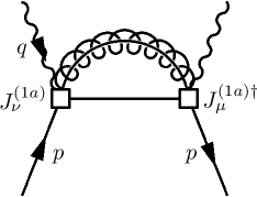
where the last expression is obtained by factorizing the usoft interactions after redefining the collinear fields. The Feynman diagram for $T_{2}(x,Q)$ is schematically shown in Fig. 5.

Figure 5: The Feynman diagram describing the forward scattering amplitude $T_{2}(x,Q)$.

Since there are no collinear particles in the $\overline{n}^{\mu}$ direction in the final state, we can define the jet function $J_{P}^{a}(\omega,n\cdot k)$ as

$$\langle 0|T\Biggl{[}\frac{1}{\overline{n}\cdot\mathcal{P}}\Bigl{[}W_{n}^{\dagger}i\hbox{\large$/$}\kern-7.27847pt\hbox{$D$}_{n}^{\perp}W_{n}\Bigr{]}\Bigl{[}\delta(\omega-\overline{n}\cdot\mathcal{P})W_{n}^{\dagger}\xi_{n}\Bigr{]}(z)\cdot\Bigl{[}\overline{\xi}_{n}W_{n}\Bigr{]}\Bigl{[}W_{n}^{\dagger}i\overleftarrow{\hbox{\large$/$}\kern-7.27847pt\hbox{$D$}_{n}^{\perp}}W_{n}\Bigr{]}\frac{1}{\overline{n}\cdot\mathcal{P}^{\dagger}}(0)\Biggr{]}|0\rangle$$

$$\equiv i\frac{\hbox{$/$}\kern-5.50117pt\hbox{$n$}}{2}\int\frac{d^{4}k}{(2\pi)^{4}}e^{-ik\cdot z}J_{P}^{a}(\omega,n\cdot k),$$ (92)

and $\hat{T}_{2}^{aa}$ can be written, with $z=\overline{n}\cdot z/2$, as

$$\hat{T}_{2}^{aa}(x,Q) = -\int d\omega d\overline{\omega}B^{2}_{a}(\omega,\overline{\omega})\int\frac{dn\cdot kdz}{2\pi}e^{i\Bigl{(}(1-w)\overline{\omega}/2-n\cdot k\Bigr{)}z}J_{P}^{a}(\omega,n\cdot k)$$

$$\times T\Bigl{[}\overline{\xi}_{\bar{n}}W_{\bar{n}}\tilde{S}_{\bar{n}}^{\dagger}S_{n}(z)\frac{\hbox{$/$}\kern-5.50117pt\hbox{$n$}}{2}S_{n}^{\dagger}S_{\bar{n}}\delta(\overline{\omega}-\mathcal{P}_{+})W_{\bar{n}}^{\dagger}\xi_{\bar{n}}(0)\Bigr{]}$$

$$= -\int d\omega d\overline{\omega}B_{a}^{2}(\omega,\overline{\omega})\int\frac{dn\cdot kdz}{2\pi}\int d\eta e^{i\Bigl{(}(1-w)\overline{\omega}/2-n\cdot k-\eta\Bigr{)}z}J_{P}^{a}(\omega,n\cdot k)$$

$$\times \frac{1}{N}\langle 0|\mathrm{tr}\Bigl{[}\tilde{S}_{\bar{n}}^{\dagger}S_{n}\delta(\eta+n\cdot i\partial)S_{n}^{\dagger}S_{\bar{n}}\Bigr{]}|0\rangle\cdot T\Bigl{[}\overline{\xi}_{\bar{n}}W_{\bar{n}}\delta(\overline{\omega}-n\cdot\mathcal{P}_{+})\frac{\hbox{$/$}\kern-5.50117pt\hbox{$n$}}{2}W_{\bar{n}}^{\dagger}\xi_{\bar{n}}\Bigr{]},$$ (94)

By putting $\eta=(1-v)n\cdot p$ ($w<v<1$), the spin-averaged matrix element between the proton state, $T_{2}^{aa}$ is given as

$$T_{2}^{aa}(x,Q) = -n\cdot P\int d\omega d\overline{\omega}B_{a}^{2}(\omega,\overline{\omega})\int d\eta S(\eta)J_{P}^{a}\Bigl{(}\omega,(1-w)\frac{\overline{\omega}}{2}-\eta\Bigr{)}$$ (95)

$$\times \int_{0}^{1}dy\delta(\overline{\omega}-2yn\cdot P)g_{P}^{q}(y)$$

$$= -\int_{x}^{1}\frac{dy}{y}g_{P}^{q}(y)\int_{w}^{1}dv\tilde{S}(v)\int d\omega B_{a}^{2}(Q,\omega)n\cdot pJ_{P}^{a}\Bigl{(}\omega,(v-w)n\cdot p\Bigr{)},$$

We can also compute the contribution to $T_{2}(x,Q)$ using $J_{\mu}^{(1b)}$, which comes from the part proportional to $n_{\mu}n_{\nu}$ in $\hat{T}_{\mu\nu}$. It is written as

$$\hat{T}_{2}^{bb}(x,Q) = i\int d^{4}ze^{i(q-\tilde{p}^{\prime}+\tilde{p})\cdot z}\int d\omega d\omega^{\prime}d\overline{\omega}B_{b}(\omega,\overline{\omega})B_{b}(\omega^{\prime},\overline{\omega})$$ (96)

$$\times T\Biggl{[}\overline{\xi}_{\bar{n}}W_{\bar{n}}\frac{1}{n\cdot\mathcal{P}^{\dagger}}\Bigl{[}W_{n}^{\dagger}i\overleftarrow{\hbox{\large$/$}\kern-7.27847pt\hbox{$D$}_{n}^{\perp}}W_{n}\Bigr{]}\Bigl{[}\delta(\omega-\overline{n}\cdot\mathcal{P})W_{n}^{\dagger}\xi_{n}\Bigr{]}(z)$$

$$\times \Bigl{[}\overline{\xi}_{n}W_{n}\delta(\omega^{\prime}-\overline{n}\cdot\mathcal{P}^{\prime})\Bigr{]}\Bigl{[}W_{n}^{\dagger}i\hbox{\large$/$}\kern-7.27847pt\hbox{$D$}_{n}^{\perp}W_{n}\Bigr{]}\delta(\overline{\omega}-\mathcal{P}_{+})\frac{1}{n\cdot\mathcal{P}}W_{\bar{n}}^{\dagger}\xi_{\bar{n}}(0)\Biggr{]}.$$

By defining the jet function $J_{P}^{b}(\omega,n\cdot k)$ as

$$\langle 0|T\Biggl{[}\Bigl{[}W_{n}^{\dagger}i\overleftarrow{\hbox{\large$/$}\kern-7.27847pt\hbox{$D$}_{n}^{\perp}}W_{n}\Bigr{]}\Bigl{[}\delta(\omega-\overline{n}\cdot\mathcal{P})W_{n}^{\dagger}\xi_{n}\Bigr{]}(z)\cdot\Bigl{[}\overline{\xi}_{n}W_{n}\Bigr{]}\Bigl{[}W_{n}^{\dagger}i\hbox{\large$/$}\kern-7.27847pt\hbox{$D$}_{n}^{\perp}W_{n}\Bigr{]}(0)\Biggr{]}|0\rangle$$

$$\equiv i\frac{\hbox{$/$}\kern-5.50117pt\hbox{$n$}}{2}\int\frac{d^{4}k}{(2\pi)^{4}}e^{-ik\cdot z}J_{P}^{b}(\omega,n\cdot k),$$ (97)

$\hat{T}_{2}^{bb}$ after factorizing the usoft interactions is given as

$$\hat{T}_{2}^{bb}(x,Q) = -\int d\omega d\overline{\omega}B_{b}^{2}(\omega,\overline{\omega})\int\frac{dn\cdot kdz}{2\pi}e^{i\Bigl{(}(1-w)\overline{\omega}/2-n\cdot k\Bigr{)}z}J_{P}^{b}(\omega,n\cdot k)$$

$$\times T\Bigl{[}\overline{\xi}_{\bar{n}}W_{\bar{n}}\tilde{S}_{\bar{n}}^{\dagger}S_{n}(z)\frac{\hbox{$/$}\kern-5.50117pt\hbox{$n$}}{2}S_{n}^{\dagger}S_{\bar{n}}\delta(\overline{\omega}-n\cdot\mathcal{P}_{+})W_{\bar{n}}^{\dagger}\xi_{\bar{n}}(0)\Bigr{]}$$

$$= -\int d\omega d\overline{\omega}B_{b}^{2}(\omega,\overline{\omega})\int\frac{dn\cdot kdz}{2\pi}\int d\eta e^{i\Bigl{(}(1-w)\overline{\omega}/2-n\cdot k-\eta\Bigr{)}z}J_{P}^{b}(\omega,n\cdot k)$$

$$\times \frac{1}{N}\langle 0|\mathrm{tr}\Bigl{(}\tilde{S}_{\bar{n}}^{\dagger}S_{n}\delta(\eta+n\cdot i\partial)S_{n}^{\dagger}S_{\bar{n}}\Bigr{)}|0\rangle\cdot\overline{\xi}_{\bar{n}}W_{\bar{n}}\frac{1}{n\cdot\mathcal{P}^{\dagger}}\frac{\hbox{$/$}\kern-5.50117pt\hbox{$n$}}{2}\delta(\overline{\omega}-n\cdot\mathcal{P}_{+})\frac{1}{n\cdot\mathcal{P}}W_{\bar{n}}^{\dagger}\xi_{\bar{n}},$$

and the spin-averaged matrix element between the proton state, $T_{2}^{bb}$, is given as

$$T_{2}^{bb}(x,Q) = -n\cdot P\int d\omega d\overline{\omega}B_{b}^{2}(\omega,\overline{\omega})\int d\eta S(\eta)J_{P}^{b}\Bigl{(}\omega,(1-w)\overline{\omega}/2-\eta\Bigr{)}$$ (99)

$$\times \frac{4}{\overline{\omega}^{2}}\int_{0}^{1}dy\delta(\overline{\omega}-2yn\cdot P)g_{P}^{q}(y)$$

$$= -\int_{x}^{1}\frac{dy}{y}g_{P}^{q}(y)\int_{w}^{1}dv\tilde{S}(v)\int d\omega\frac{B_{b}^{2}(Q,\omega)}{n\cdot p}J_{P}^{b}\Bigl{(}\omega,(v-w)n\cdot p\Bigr{)}.$$

We can clearly see that both $T_{2}^{aa}$ and $T_{2}^{bb}$ factorize. By taking the imaginary part of $T_{2}^{aa}$ or $T_{2}^{bb}$, the longitudinal structure function $F_{L}(x,Q)$ can be written as

$$F_{L}(x,Q) = 8\int_{x}^{1}\frac{dy}{y}g_{P}^{q}(y)\int_{w}^{1}dv\tilde{S}(v)\int d\omega B_{a}^{2}(Q,\omega)n\cdot p\Bigl{[}\frac{-1}{\pi}\mathrm{Im}J_{P}^{a}\Bigl{(}\omega,(v-w)n\cdot p\Bigr{)}\Bigr{]},$$

$$F_{L}(x,Q) = 8\int_{x}^{1}\frac{dy}{y}g_{P}^{q}(y)\int_{x}^{1}dv\tilde{S}(v)\int d\omega\frac{B_{b}^{2}(Q,\omega)}{n\cdot p}\Bigl{[}\frac{-1}{\pi}\mathrm{Im}J_{P}^{b}\Bigl{(}\omega,(v-w)n\cdot p\Bigr{)}\Bigr{]},$$ (100)

where the first (second) expression is obtained using $T_{2}^{aa}$ ($T_{2}^{bb}$).

Figure 6: Feynman rules of the current $j^{(1b)}(\omega)$ with one or two $n$-collinear gluons.

Figure 7: Feynman rules of the current $j^{(1a)}(\omega)$ with a single $n$-collinear gluon.

The jet function $J_{P}^{b}(\omega,n\cdot k)$ at order $\alpha_{s}$ can be computed from Eq. (VIII). The Feynman rules for $j^{(1b)}$ with one or two collinear gluons in the $n^{\mu}$ direction are shown in Fig. 6. And the matrix element $M_{b}$ from Fig. 5 with $J_{\mu}^{(1b)}$, after extracting the overall factor $1/(n\cdot p)^{2}$, is given as

$$M_{b} = g^{2}C_{F}\int\frac{d^{D}l}{(2\pi)^{D}}\gamma_{\perp\alpha}\delta\Bigl{(}\omega-\overline{n}\cdot(l+p^{\prime})\Bigr{)}\frac{\hbox{$/$}\kern-5.50117pt\hbox{$n$}}{2}\frac{\overline{n}\cdot(l+p^{\prime})}{(l+p^{\prime})^{2}}\gamma_{\perp}^{\alpha}\frac{1}{l^{2}}$$ (101)

$$= -g^{2}C_{F}\frac{\hbox{$/$}\kern-5.50117pt\hbox{$n$}}{2}(D-2)\int\frac{d^{D}l}{(2\pi)^{D}}\delta\Bigl{(}\omega-\overline{n}\cdot(l+p^{\prime})\Bigr{)}\frac{\overline{n}\cdot(l+p^{\prime})}{l^{2}(l+p^{\prime})^{2}}$$

$$\longrightarrow i\frac{\hbox{$/$}\kern-5.50117pt\hbox{$n$}}{2}\frac{\alpha_{s}C_{F}}{2\pi}\frac{\omega}{\overline{n}\cdot p^{\prime}}\theta(\omega)\theta(\overline{n}\cdot p^{\prime}-\omega)\Bigl{[}1+\ln\frac{\omega(\overline{n}\cdot p^{\prime}-\omega)(-n\cdot k-i\epsilon)}{\overline{n}\cdot p^{\prime}\mu^{2}}\Bigr{]},$$

where we collect the finite terms only in the last expression. Here $\overline{n}\cdot p^{\prime}$ is the total collinear momentum of the intermediate states, and can be replaced by $\overline{n}\cdot q=Q$. Therefore the jet function $J_{P}^{b}(\omega,n\cdot k)$ is given by

$$J_{P}^{b}(\omega,n\cdot k)=\frac{\alpha_{s}C_{F}}{2\pi}\frac{\omega}{Q}\theta(\omega)\theta(Q-\omega)\Bigl{[}1+\ln\frac{\omega(Q-\omega)(-n\cdot k-i\epsilon)}{Q\mu^{2}}\Bigr{]}.$$ (102)

Comparing the definitions of $J_{P}^{a}$ and $J_{P}^{b}$ in Eqs. (VIII) and (VIII), $J_{P}^{a}(\omega,n\cdot k)$ is given by

$$J_{P}^{a}(\omega,n\cdot k)=\frac{1}{Q^{2}}J_{P}^{b}(\omega,n\cdot k).$$ (103)

It is easy to see this relation by looking at the Feynman rules for $j^{(1a)}$, which are presented in Fig. 7. Note that there is an additional factor of $1/(\overline{n}\cdot p^{\prime})^{2}$ in the definition of $J_{P}^{a}$, and the nonzero contribution comes from the part proportional to $\gamma_{\perp\alpha}$, of which the radiative corrections are the same using either $j^{(1a)}$ or $j^{(1b)}$.

Let us simplify the expression for $F_{L}(x,Q)$ in Eq. (VIII). At order $\alpha_{s}$, since the jet functions are already at order $\alpha_{s}$, the Wilson coefficients $C(Q)$ and $B_{a,b}(\omega)$ take their tree-level values, that is, 1. Introducing the dimensionless variable $r=\omega/Q$, the jet function $J_{P}^{b}$ is written as

$$J_{P}^{b}\Bigl{(}(v-w)n\cdot p\Bigr{)}=\frac{\alpha_{s}C_{F}}{2\pi}r\theta(r)\theta(1-r)\Bigl{\{}1+\ln\Bigr{[}\frac{Q^{2}}{\mu^{2}}r(1-r)\Bigl{(}-(1-\frac{v}{w})-i\epsilon\Bigr{)}\Bigr{]}\Bigr{\}}.$$ (104)

Therefore the imaginary part is given by

$$\overline{J}_{P}^{b}\Bigl{(}r,\frac{w}{v}\Bigr{)}\equiv-\frac{1}{\pi}\mathrm{Im}J_{P}^{b}\Bigl{(}(v-w)n\cdot p\Bigr{)}=\frac{\alpha_{s}C_{F}}{2\pi}r\theta(r)\theta(1-r).$$ (105)

At order $\alpha_{s}$, the longitudinal structure function $F_{L}(x,Q)$ becomes

$$F_{L}(x,Q)=8\frac{\alpha_{s}C_{F}}{4\pi}\int_{x}^{1}\frac{dy}{y}g_{P}^{q}(y)\frac{1}{w}\int_{w}^{1}dv\tilde{S}(v)=8\frac{\alpha_{s}C_{F}}{4\pi}\int_{x}^{1}\frac{dy}{y}g_{P}^{q}(y)\int_{w}^{1}dvw\tilde{S}(v),$$ (106)

where the first (second) expression comes from $T_{2}^{aa}$ ($T_{2}^{bb}$). The two expressions differ by a factor of $w^{2}$, which gives a subleading correction since $1-w\sim\Lambda/Q$. Therefore the contributions from $T_{2}^{aa}$ and $T_{2}^{bb}$ to $F_{L}(x,Q)$ are the same near the endpoint region at leading order in $\Lambda/Q$. In fact, the result of the electromagnetic current conservation goes further than the fact that $T_{2}$ can be obtained using either $J_{\mu}^{(1a)}$ and $J_{\mu}^{(1b)}$. It should hold to all orders in $\alpha_{s}$, and the scaling behavior of the two currents should also be the same. We present the anomalous dimensions for $J_{\mu}^{(1b)}$ at one loop in Appendix C.

The moment of $F_{L}(x,Q)$ using the first expression in Eq. (VIII) is written as

$$F_{L,n}(Q) = \int_{0}^{1}dxx^{n-1}F_{L}(x,Q)$$ (107)

$$= \frac{2\alpha_{s}C_{F}}{\pi}\int_{0}^{1}dxx^{n-1}\int_{0}^{1}dyg_{P}^{q}(y)\int_{0}^{1}dw\delta(x-wy)\frac{1}{w}\int_{w}^{1}dv\tilde{S}(v)$$

$$= \frac{2\alpha_{s}C_{F}}{\pi}\int_{0}^{1}dyy^{n-1}g_{P}^{q}(y)\int_{0}^{1}dww^{n-2}\int_{w}^{1}\frac{dv}{v}v\tilde{S}(v)$$

$$= \frac{2\alpha_{s}C_{F}}{\pi}\int_{0}^{1}dyy^{n-1}g_{P}^{q}(y)\int_{0}^{1}dww^{n-2}\int_{0}^{1}du\int_{0}^{1}dv\delta(w-vu)v\tilde{S}(v)$$

$$= \frac{2\alpha_{s}C_{F}}{\pi}\frac{1}{n-1}\int_{0}^{1}dyy^{n-1}g_{P}^{q}(y)\int_{0}^{1}dvv^{n-1}\tilde{S}(v)$$

$$\longrightarrow \frac{2\alpha_{s}C_{F}}{\pi}\frac{1}{n}g_{P,n}^{q}\cdot\tilde{S}_{n}=\frac{2\alpha_{s}C_{F}}{\pi}\frac{1}{n}f_{P,n,n+1}^{q},$$

where the last expression is obtained in the large $n$ limit. Compared to the moment $F_{1,n}$, $F_{L,n}$ is suppressed by $n$, which confirms that the longitudinal structure function $F_{L}(x,Q)$ is suppressed by $\Lambda/Q$ compared to $F_{1}(x,Q)$. In order to obtain the exponentiated form, we should compute the radiative corrections to next-to-leading order accuracy. This has not been done here, but all the logarithmic terms such as $\alpha_{s}^{k}\ln^{l}n/n$ can be resummed from the factorization property in SCET, as suggested in the approach using the full theory Akhoury:1998gs .

IX Conclusion

DIS near the endpoint region can be described in SCET. The factorization of the structure functions is explicitly shown to order $\alpha_{s}$, and the moments of the structure functions are expressed as a product of the Wilson coefficients, the moments of the jet functions, the collinear matrix elements, and the soft Wilson lines. The radiative corrections for each component can be separately computed using perturbation theory. The structure function $F_{1}(x,Q)$ starts at leading order in $\Lambda$, while the longitudinal structure function $F_{L}(x,Q)$ starts from order $\Lambda$ and $\alpha_{s}$. Therefore the Callan-Gross sum rule holds at leading order in $\Lambda$, and the corrections can be systematically computed in SCET.

High-energy processes, such as DIS, Drell-Yan processes, hadron collisions, $e^{+}e^{-}\rightarrow$ jets, can be described by SCET. And all these processes possess common features though the detailed dynamics are different. First, the scattering cross sections are factorized, and the short-distance physics and the long-distance physics are separated. There is a universal soft Wilson line describing soft gluon emissions near the endpoint region with the appropriate prescription for the soft Wilson lines depending on the external collinear particles. And there is a contribution from the parton distribution functions if the initial particles are hadrons.

Compared to the approach in full QCD css , there is advantage in employing SCET in DIS near the endpoint region. First, the factorization property becomes transparent since SCET is formulated from the beginning to decouple the collinear and the soft degrees of freedom. And the power counting in powers of $\Lambda$ can be systematically performed. Secondly, once the factorized form is given, each factor has a different physical origin and its radiative corrections and evolutions can be computed in perturbation theory. The hard coefficient $C(Q,\mu_{0})$ comes from the hard physics of order $Q$ and can be computed in matching the full theory and $\mathrm{SCET}_{\mathrm{I}}$. The jet function $J_{P}$ arises from the hard-collinear physics of order $\sqrt{Q\Lambda}$, and can be computed by matching $\mathrm{SCET}_{\mathrm{I}}$ and $\mathrm{SCET}_{\mathrm{II}}$. The soft Wilson lines and the collinear matrix elements are combined to give the parton distribution functions. Since the collinear particles and the soft particles are decoupled, the radiative corrections for the soft Wilson line are governed only by the soft interactions in $\mathrm{SCET}_{\mathrm{II}}$, while those for the collinear matrix elements are governed only by the collinear interactions. To guarantee this, and to avoid double counting, the zero-bin subtraction should be performed. Each contribution is clearly separated and SCET specifies the prescription for computing radiative corrections.

In this paper we have considered the flavor nonsinglet structure functions. To be complete, the flavor singlet structure functions should be included. In this case we have to consider the collinear operators with gluons, which contribute to the gluon distribution function in the proton. Though it will be more involved because of the operator mixing, the procedure for showing the factorization is straightforward. The complete treatment of DIS near the endpoint region including the flavor singlet structure function will be considered elsewhere. It will be interesting to see if other various high-energy processes near the endpoint region can have similar features as those in DIS.

Note added: The original preprint version of this paper did not include the zero-bin contribution Manohar:2006nz , and the parton distribution function in SCET was not properly defined excluding the soft part. In this paper, the zero-bin subtraction is correctly performed to solve the double counting problem, and the parton distribution function is carefully defined in the endpoint region. Because of these, the results of the calculations and the conclusion of the paper have changed. However, in the meantime, several authors Becher:2006mr ; Chen:2006vd criticized this paper based on the original preprint version. We would like to comment on the criticism which appeared in the literature.

In Ref. Becher:2006mr , the authors argue that there should be no extra soft contributions outside the parton distribution function, which is correct based on the original preprint. However, in this paper, we include the soft contributions as part of the parton distribution function, which also affects the jet function in the endpoint region, contrary to the case away from the endpoint. They also claim that the $\overline{n}$-collinear gluon exchange shown in Fig. 8 (b), (c) are not kinematically allowed. But all the $\overline{n}$-collinear contributions in Fig. 8 should be included because the interaction of the collinear gluon with the quark happens inside the proton, and the resulting momentum of the quark undergoing the hard collision should be regarded as $n$ collinear, not the momentum of the quark before it interacts with a collinear gluon. The detail is explained in Appendix A.

The main criticism of Ref. Chen:2006vd is that the double counting problem is not performed properly, and that the parton distribution function is not correctly identified if only the matrix elements of the collinear operators are included. In the current paper, the double counting is treated using the zero-bin subtraction method. For the parton distribution function, we include the effect of the soft gluons in the parton distribution function. Besides these, we agree with their claim that the structure function depends only on $Q^{2}$, and $(1-x)Q^{2}$, not on $(1-x)^{2}Q^{2}$, which is illustrated clearly in Eq. (48), where the structure function depends only on $Q^{2}$ and $\mu_{0}^{2}=(1-x)Q^{2}$, and the dependence on $\mu$ cancels.

Appendix A Zero-bin subtraction before the usoft factorization

For the purpose of illustrating the zero-bin subtraction method in $\mathrm{SCET}_{\mathrm{I}}$, we consider the radiative corrections to the forward scattering amplitude before the usoft factorization. The starting point is that $\hat{T}_{\mu\nu}^{(0)}$ from Eq. (27) is given by

$$\hat{T}^{(0)}_{\mu\nu} = iC^{2}(Q)\int d^{4}ze^{i(q+\tilde{p}-\tilde{p}^{\prime})\cdot z}T\Bigl{[}J_{\mu}^{(0)\dagger}(z)J_{\nu}^{(0)}(0)\Bigr{]}$$ (108)

$$= iC^{2}(Q)\int d^{4}ze^{i(q+\tilde{p}-\tilde{p}^{\prime})\cdot z}T\Bigl{[}\overline{\xi}_{\bar{n}}W_{\bar{n}}\gamma_{\mu}W_{n}^{\dagger}\xi_{n}(z)\overline{\xi}_{n}W_{n}\gamma_{\nu}W_{\bar{n}}^{\dagger}\xi_{\bar{n}}(0)\Bigr{]},$$

where the collinear field is not redefined by Eq. (25), and can interact with usoft gluons.

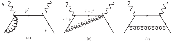
We consider the radiative corrections with the $\overline{n}$-collinear gluons, which contribute to the renormalization of the quark distribution functions. The Feynman diagrams are shown in Fig. 8. We consider the amplitudes only at the parton level,and the convolution with the parton distribution function is straightforward. The naive contributions proportional to $-g^{\perp}_{\mu\nu}$ from Fig. 8 (a), (b) with their mirror images and (c) are given as

$$M_{a} = 4ig^{2}C_{F}\frac{\hbox{$/$}\kern-5.50117pt\hbox{$n$}}{2}\frac{1}{n\cdot p^{\prime}}\int\frac{d^{D}l}{(2\pi)^{D}}\frac{n\cdot(l+p)}{l^{2}(l+p)^{2}n\cdot l},$$

$$M_{b} = -4ig^{2}C_{F}\frac{\hbox{$/$}\kern-5.50117pt\hbox{$n$}}{2}\int\frac{d^{D}l}{(2\pi)^{D}}\frac{n\cdot(l+p)}{l^{2}(l+p)^{2}n\cdot(l+p^{\prime})n\cdot l},$$

$$M_{c} = ig^{2}C_{F}\frac{\hbox{$/$}\kern-5.50117pt\hbox{$n$}}{2}\int\frac{d^{D}l}{(2\pi)^{D}}\frac{1}{l^{2}[(l+p)^{2}]^{2}n\cdot(l+p^{\prime})}\gamma_{\perp\alpha}\hbox{$/$}\kern-4.09029pt\hbox{$l$}_{\perp}\hbox{$/$}\kern-4.09029pt\hbox{$l$}_{\perp}\gamma_{\perp}^{\alpha},$$ (109)

where $p^{\prime}_{\mu}=p_{\mu}+q_{\mu}$ is the $n$-collinear momentum, and we put $p_{\perp}=0$ for simplicity.

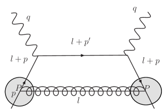
Figure 8: Feynman diagrams of the contribution from collinear gluons to the forward scattering amplitude in $\rm{SCET_{I}}$. The mirror images of (a) and (b) are omitted.

Figure 9: When an $\overline{n}$ gluon is exchanged, there is a kinematical region where the initial state with $l+p$ is $\overline{n}$ collinear, and the intermediate state with $l+p^{\prime}$ is $n$ collinear, while the loop momentum $l$ is $\overline{n}$ collinear.

Note that in $M_{b}$, the propagators are written in such a way that $l+p^{\prime}$ is collinear in the $n$ direction. This should be included in the collinear contribution, contrary to the claim in Ref. Becher:2006mr , in which the authors claim that Fig. 8 (b), and (c) should not be included since they are kinematically forbidden. However, by looking into the kinematics carefully, there are collinear contributions from Fig. 8 (b), and (c). The point is that a quark inside the proton can interact with $\overline{n}$-collinear gluons before the hard collision. Therefore the $\overline{n}$-collinear gluon is regarded as part of the proton, and forms an $\overline{n}$ collinear jet. The parton distribution function describes the partons which undergo a hard collision after all the interactions with the collinear jet.

The situation is schematically shown in Fig. 9, which is Fig. 8 (c). The collinear quark interacts with a collinear gluon before it collides with a hard photon. Therefore the longitudinal momentum of the collinear quark for the hard collision is $n\cdot(l+p)$, not $n\cdot p$, where $n\cdot p$ is the longitudinal momentum fraction before it interacts with a collinear gluon. In order to see if the $\overline{n}$-collinear gluon is allowed by kinematics, let us introduce the partonic variable $w^{\prime}$, to avoid confusion, which is given by

$$w^{\prime}\sim-\frac{n\cdot q}{n\cdot(l+p)}.$$ (110)

And $n\cdot(l+p)$ and $n\cdot(l+p^{\prime})$ are given by

$$n\cdot(l+p)=Q/w^{\prime},\ \ n\cdot(l+p^{\prime})=n\cdot(l+p+q)=(1-w^{\prime})n\cdot(l+p)=\frac{1-w^{\prime}}{w^{\prime}}Q.$$ (111)

In the endpoint region where $w^{\prime}\rightarrow 1$, $l+p$ can be $\overline{n}$ collinear, $l+p^{\prime}$ can be $n$ collinear, while $l$ is $\overline{n}$ collinear. Therefore the contribution from $\overline{n}$-collinear gluons should be included.

The reason why Eq. (A) is naive is because the loop momentum can be soft, which should be avoided in the collinear sector. Therefore we subtract the contribution where the loop momentum becomes soft, and we call this the zero-bin contribution. It can be obtained from Eq. (A) by power counting, where all the components of the loop momentum $l^{\mu}$ scales as $\Lambda$. The zero-bin amplitudes are given as

$$M_{a}^{0} = 4ig^{2}C_{F}\frac{\hbox{$/$}\kern-5.50117pt\hbox{$n$}}{2}\frac{1}{n\cdot p^{\prime}}\int\frac{d^{D}l}{(2\pi)^{D}}\frac{n\cdot p}{l^{2}(n\cdot p\overline{n}\cdot l+p^{2})n\cdot l},$$

$$M_{b}^{0} = -4ig^{2}C_{F}\frac{\hbox{$/$}\kern-5.50117pt\hbox{$n$}}{2}\int\frac{d^{D}l}{(2\pi)^{D}}\frac{n\cdot p}{l^{2}(n\cdot p\overline{n}\cdot l+p^{2})n\cdot(l+p^{\prime})n\cdot l},$$ (112)

where we put $p^{2}$ to regulate the infrared divergence. And the zero-bin contribution from Fig. 8 (c) is suppressed, and we neglect it here. The total zero-bin contribution is given as

$$M_{a}^{0}+M_{b}^{0} = 4ig^{2}C_{F}\frac{\hbox{$/$}\kern-5.50117pt\hbox{$n$}}{2}\int\frac{d^{D}l}{(2\pi)^{D}}\frac{n\cdot p}{l^{2}(n\cdot p\overline{n}\cdot l+p^{2})n\cdot l}\Bigl{[}\frac{1}{n\cdot p^{\prime}}-\frac{1}{n\cdot(l+p^{\prime})}\Bigr{]}$$ (113)

$$= 4ig^{2}C_{F}\frac{\hbox{$/$}\kern-5.50117pt\hbox{$n$}}{2}\frac{1}{n\cdot p^{\prime}}\int\frac{d^{D}l}{(2\pi)^{D}}\frac{n\cdot p}{l^{2}(n\cdot p\overline{n}\cdot l+p^{2})n\cdot(l+p^{\prime})}.$$

Figure 10: Feynman diagram of the contribution from usoft gluons to the forward scattering amplitude in $\rm{SCET_{I}}$, and the mirror image is omitted.

The usoft contributions from Fig. 10 are given by

$$M_{us}=4ig^{2}C_{F}\frac{\hbox{$/$}\kern-5.50117pt\hbox{$n$}}{2}\frac{1}{n\cdot p^{\prime}}\int\frac{d^{D}l}{(2\pi)^{D}}\frac{n\cdot p}{l^{2}(n\cdot p\overline{n}\cdot l+p^{2})n\cdot(l+p^{\prime})},$$ (114)

which is exactly equal to the zero-bin contribution. Therefore the correct computation including the zero-bin subtraction becomes

$$M_{a}+M_{b}+M_{c}-(M_{a}^{0}+M_{b}^{0})+M_{us}=M_{a}+M_{b}+M_{c},$$ (115)

which states that the naive collinear contribution without the zero-bin subtraction gives the correct result. It is also true in $\mathrm{SCET}_{\mathrm{II}}$ after the soft factorization. The zero-bin contribution to the collinear operator is the same as the radiative correction to the soft Wilson line.

In calculating $M_{a}+M_{b}$, note that we can write $M_{b}$ as

$$M_{b} = -4ig^{2}C_{F}\frac{\hbox{$/$}\kern-5.50117pt\hbox{$n$}}{2}\int\frac{d^{D}l}{(2\pi)^{D}}\frac{n\cdot(l+p)}{l^{2}(l+p)^{2}n\cdot(l+p^{\prime})n\cdot l}$$ (116)

$$= -4ig^{2}C_{F}\frac{\hbox{$/$}\kern-5.50117pt\hbox{$n$}}{2}\frac{1}{n\cdot p^{\prime}}\int\frac{d^{D}l}{(2\pi)^{D}}\Bigl{[}\frac{n\cdot(l+p)}{l^{2}(l+p)^{2}n\cdot l}-\frac{n\cdot(l+p)}{l^{2}(l+p)^{2}n\cdot(l+p^{\prime})}\Bigr{]},$$

where the first term is equal to $-M_{a}$. Therefore $M_{a}+M_{b}$ is given as

$$M_{a}+M_{b}=4ig^{2}C_{F}\frac{\hbox{$/$}\kern-5.50117pt\hbox{$n$}}{2}\frac{1}{n\cdot p^{\prime}}\int\frac{d^{D}l}{(2\pi)^{D}}\frac{n\cdot(l+p)}{l^{2}(l+p)^{2}n\cdot(l+p^{\prime})}.$$ (117)

Evaluating the $\overline{n}\cdot l$ integral by contours, doing the ${\bf l}_{\perp}$ integral, and using the substitution $n\cdot l=-zn\cdot p$ gives the infinite part

$$M_{a}+M_{b} = -\frac{\alpha_{s}C_{F}}{\pi}\frac{1}{\epsilon}\frac{\hbox{$/$}\kern-5.50117pt\hbox{$n$}}{2}\frac{1}{n\cdot p}\int_{0}^{1}dz\frac{1-z}{(1-w+i0^{+})(1-z-w+i0^{+})}$$ (118)

$$= -\frac{\alpha_{s}C_{F}}{\pi}\frac{1}{\epsilon}\frac{\hbox{$/$}\kern-5.50117pt\hbox{$n$}}{2}\frac{1}{n\cdot p}\frac{1}{1-w+i0^{+}}\Bigl{(}1+w\ln\frac{1-w+i0^{+}}{-w+i0^{+}}\Bigr{)},$$

where $n\cdot p^{\prime}=(1-w)n\cdot p$. Similarly, $M_{c}$ is given as

$$M_{c} = -\frac{\alpha_{s}C_{F}}{2\pi}\frac{1}{\epsilon}\frac{\hbox{$/$}\kern-5.50117pt\hbox{$n$}}{2}\frac{1}{n\cdot p}\int_{0}^{1}dz\frac{z}{1-w-z+i0^{+}}$$ (119)

$$= -\frac{\alpha_{s}C_{F}}{2\pi}\frac{1}{\epsilon}\frac{\hbox{$/$}\kern-5.50117pt\hbox{$n$}}{2}\frac{1}{n\cdot p}\Bigl{(}1+(1-w)\ln\frac{1-w+i0^{+}}{-w+i0^{+}}\Bigr{)}.$$

And the wave function renormalization for the external quarks is given as

$$M_{\mathrm{w.f.}}=\frac{\alpha_{s}C_{F}}{4\pi}\frac{1}{\epsilon}\frac{1}{n\cdot p}\frac{\hbox{$/$}\kern-5.50117pt\hbox{$n$}}{2}\frac{1}{1-w+i0^{+}}.$$ (120)

Noting that

$$\mathrm{Im}\,\frac{w}{1-w+i0^{+}}\ln(w-1-i0^{+})=-\pi\frac{w}{(1-w)_{+}},\ \mathrm{Im}\,\frac{1}{1-w+i0^{+}}=-\pi\delta(1-w),$$ (121)

we obtain

$$\frac{1}{\pi}\mathrm{Im}\,(M_{a}+M_{b}+M_{c}+M_{\mathrm{w.f.}})=\frac{\alpha_{s}C_{F}}{2\pi}\frac{1}{\epsilon}\frac{1}{n\cdot p}\frac{\hbox{$/$}\kern-5.50117pt\hbox{$n$}}{2}\Bigl{(}\frac{3}{2}\delta(1-w)+\frac{1+w^{2}}{(1-w)_{+}}\Bigr{)}.$$ (122)

The tree-level amplitude is given by

$$M_{\mathrm{tree}}=-\frac{1}{n\cdot p}\frac{\hbox{$/$}\kern-5.50117pt\hbox{$n$}}{2}\frac{1}{1-w+i0^{+}},$$ (123)

the imaginary part of which is

$$\frac{1}{\pi}\mathrm{Im}\,M_{\mathrm{tree}}=\frac{1}{n\cdot p}\frac{\hbox{$/$}\kern-5.50117pt\hbox{$n$}}{2}\delta(1-w).$$ (124)

Adding Eqs. (122) and (124), we have

$$\frac{1}{n\cdot p}\frac{\hbox{$/$}\kern-5.50117pt\hbox{$n$}}{2}\Bigl{[}\delta(1-w)+\frac{\alpha_{s}C_{F}}{2\pi}\frac{1}{\epsilon}\Bigl{(}\frac{3}{2}\delta(1-w)+\frac{1+w^{2}}{(1-w)_{+}}\Bigr{)}\Bigr{]},$$ (125)

from which the anomalous dimension is given as

$$\gamma=-\frac{\alpha_{s}C_{F}}{\pi}\Bigl{(}\frac{3}{2}\delta(1-w)+\frac{1+w^{2}}{(1-w)_{+}}\Bigr{)},$$ (126)

which is exactly the Altarelli-Parisi kernel. Note that this is the result including the zero-bin subtraction, and it corresponds to the radiative corrections for the sum of the collinear matrix element and the soft part.

Appendix B Discontinuity in $\mathrm{SCET}_{\mathrm{I}}$ and $\mathrm{SCET}_{\mathrm{II}}$

It is possible to take the imaginary part of the forward scattering amplitude to obtain the structure function in $\mathrm{SCET}_{\mathrm{I}}$ as well as in $\mathrm{SCET}_{\mathrm{II}}$. If we only consider the collinear interactions with the intermediate state, the computation produces the jet function and the discontinuity due to the collinear interactions is the same both in $\mathrm{SCET}_{\mathrm{I}}$ and $\mathrm{SCET}_{\mathrm{II}}$. Therefore the issue here is how to take the discontinuity related to the (u)soft interactions. We consider the (u)soft interactions with the intermediate state in both effective theories and show that the discontinuity is the same. Since we are interested in computing the anomalous dimension of the soft Wilson line, we focus on the ultraviolet divergent part.

Figure 11: Feynman diagrams for computing the radiative corrections of the (u)soft Wilson line in (a) $\mathrm{SCET}_{\mathrm{I}}$ and (b) $\mathrm{SCET}_{\mathrm{II}}$.

Let us consider the usoft interactions in $\mathrm{SCET}_{\mathrm{I}}$ and take the discontinuity. The relevant Feynman diagrams are shown in Fig. 11 (a), where the curly lines are soft gluons. Using the dimensional regularization, the Feynman diagrams in Fig. 11 (a) are given as

$$M_{a}=-4ig^{2}C_{F}O_{\bar{n}}\int\frac{d^{D}l}{(2\pi)^{D}}\frac{1}{(l^{2}+i0^{+})\Bigl{(}\overline{n}\cdot(l+p)+i0^{+}\Bigr{)}\Bigl{(}n\cdot(l+p^{\prime})+i0^{+}\Bigr{)}(n\cdot p^{\prime}+i0^{+})},$$ (127)

where $O_{\bar{n}}$ is the operator

$$O_{\bar{n}}=\overline{\xi}_{\bar{n}}W_{\bar{n}}\gamma_{\mu}\frac{\hbox{$/$}\kern-5.50117pt\hbox{$n$}}{2}\gamma_{\nu}W_{\bar{n}}^{\dagger}\xi_{\bar{n}},$$ (128)

Evaluating the $\overline{n}\cdot l$ integral by contours, doing the ${\bf l}_{\perp}$ integral give the infinite part

$$M_{a}=\frac{\alpha_{s}C_{F}}{\pi\epsilon}\frac{O_{\bar{n}}}{n\cdot p^{\prime}+i0^{+}}\int_{-\infty}^{0}dn\cdot l\frac{1}{n\cdot(l+p^{\prime}+i0^{+})}.$$ (129)

By putting $n\cdot p^{\prime}=n\cdot(p+q)=(1-w)n\cdot p$ and $n\cdot l=-zn\cdot p$, we obtain

$$M_{a}=\frac{\alpha_{s}C_{F}}{\pi\epsilon}\frac{O_{\bar{n}}}{n\cdot p}\frac{1}{1-w+i0^{+}}\int_{0}^{1}dz\frac{1}{1-w-z+i0^{+}}=\frac{\alpha_{s}C_{F}}{\pi\epsilon}\frac{O_{\bar{n}}}{n\cdot p}\frac{\ln(w-1-i0^{+})}{1-w+i0^{+}},$$ (130)

where we neglect the $\ln w$ term as $w\rightarrow 1$. The discontinuity in $\mathrm{SCET}_{\mathrm{I}}$ from the usoft interactions is given by

$$\frac{1}{\pi}\mathrm{Im}\,M_{a}=-\frac{\alpha_{s}C_{F}}{\pi\epsilon}\frac{1}{(1-w)_{+}}\frac{O_{\bar{n}}}{n\cdot p}.$$ (131)

This analysis is similar to the analysis in Ref. Manohar:2003vb , in which a single-step matching was performed.

In $\mathrm{SCET}_{\mathrm{II}}$, the Feynman diagram is shown in Fig. 11 (b). It gives

$$M_{b}=\int d\eta\frac{1}{(1-w)n\cdot p-\eta+i0^{+}}\frac{\alpha_{s}C_{F}}{\pi\epsilon}\frac{\theta(\eta)}{\eta_{+}}O_{\bar{n}},$$ (132)

where the first term in the denominator is the coefficient (jet function at tree level) with the energy transfer $\eta$ to the soft gluon. The remaining part is the result of the soft loop calculation  Chay:2004zn . Taking the imaginary part of $M_{b}$, we have

$$\frac{1}{\pi}\mathrm{Im}\,M_{b}=-\frac{\alpha_{s}C_{F}}{\pi\epsilon}\frac{1}{(1-w)_{+}}\frac{O_{\bar{n}}}{n\cdot p},$$ (133)

which is the same result as Eq. (131) obtained in $\mathrm{SCET}_{\mathrm{I}}$.

Appendix C Anomalous dimension of $J_{\mu}^{(1b)}$

We present the calculation of the anomalous dimension for $J_{\mu}^{(1b)}$ at one loop, and explain why it is the same for $J_{\mu}^{(1a)}$. The current $J_{\mu}^{(1b)}$ from Eq. (VIII) is given as

$$J_{\mu}^{(1b)}=-n_{\mu}\int d\omega B_{b}(\omega)\Bigl{[}\overline{\xi}_{n}W_{n}\delta(\omega-\overline{n}\cdot\mathcal{P}^{\dagger})\Bigr{]}\Bigl{[}W_{n}^{\dagger}i\hbox{\large$/$}\kern-7.27847pt\hbox{$D$}_{n}^{\perp}W_{n}\Bigr{]}\frac{1}{n\cdot\mathcal{P}}W_{\bar{n}}^{\dagger}\xi_{\bar{n}}=-n_{\mu}j^{(1b)},$$ (134)

where $B_{b}(\omega)$ is the Wilson coefficient, which is 1 at tree level. The Feynman rules for $j^{(1b)}$ is given in Fig. 6, and the Feynman diagrams for the radiative corrections are given in Fig. 12. In Fig. 12, diagrams (a) to (e) are the radiative corrections from the $n$-collinear loop diagrams. Diagram (f) is from the $\overline{n}$-collinear loop diagram, and diagrams (g), (h) are the contributions from the soft loops. We employ the background gauge field method for the triple-gluon vertex, and use the dimensional regularization with $D=4-2\epsilon$. The external momenta $p^{2}$, $p^{\prime 2}$ and $q^{2}$ are kept to give infrared cutoff, and the poles in $1/\epsilon$ are of the ultraviolet origin.

Figure 12: Feynman diagrams for the radiative corrections of $j^{(1b)}(\omega)$ in $\rm{SCET_{I}}$ at one loop. $p$ is in the $\overline{n}^{\mu}$ direction, and $p^{\prime}$, $q$ are in the $n^{\mu}$ direction ($q$ incoming). Diagrams (a) to (e) include $n$-collinear loop, (f) includes the $\overline{n}$-collinear loop, and (g), (h) are the soft corrections.

Considering the flow of momenta, $p^{\prime}-q$ is the total outgoing collinear momentum in the $n^{\mu}$ direction, and $\overline{n}\cdot(p^{\prime}-q)=Q$ is the large scale in DIS. We use the variables

$$\overline{n}\cdot(p^{\prime}-q)=Q,\ \overline{n}\cdot p^{\prime}=\omega^{\prime}=Qv,\ \overline{n}\cdot q=\omega^{\prime}-Q=(1-v)Q,\ \omega=uQ,$$ (135)

and the allowed kinematic regions in DIS is $Q\geq\omega>0$. We extract the terms proportional to $\gamma_{\perp\mu}$, and the divergent terms from each category ($n$ collinear, $\overline{n}$ collinear, and soft) using the dimensionless variables are given as

$$iM_{n} = i(M_{a}+M_{b}+M_{c}+M_{d}+M_{e})$$

$$= \Gamma_{\mu}\Biggl{[}\delta(u-v)\Bigl{\{}2C_{F}\Bigl{(}\frac{1}{\epsilon^{2}}+\frac{1}{\epsilon}\Bigr{)}-\frac{N}{\epsilon}\Big{(}\ln\frac{-q^{2}}{\mu^{2}}+\ln u(1-u)\Bigr{)}+\frac{1}{N\epsilon}\ln\frac{-p^{\prime 2}}{\mu^{2}}\Bigr{\}}$$

$$+\frac{N}{\epsilon}\Bigl{\{}\Bigl{(}\frac{1-u-v}{1-v}-u\Bigl{)}\theta(u-v)+\Bigl{(}\frac{u(1-u-v)}{(1-u)v}-u\Bigr{)}\theta(v-u)$$

$$+\frac{\theta(u-v)}{(u-v)_{+}}+\frac{u}{v}\frac{\theta(v-u)}{(v-u)_{+}}\Bigr{\}}$$

$$+\frac{1}{N\epsilon}\Bigl{\{}\Bigl{(}\frac{u(1-u-v)}{(1-u)(1-v)}+x\Bigr{)}\theta(1-u-v)+\frac{(1-u)(1-v)}{v}\theta(u+v-1)\Bigr{\}}\Biggr{]},$$

$$iM_{\bar{n}} = iM_{f}=\Gamma_{\mu}C_{F}\delta(u-v)\Bigl{(}\frac{2}{\epsilon^{2}}-\frac{2}{\epsilon}\ln\frac{-p^{2}}{\mu^{2}}+\frac{2}{\epsilon}\Bigr{)},$$

$$iM_{s} = i(M_{g}+M_{h})=\Gamma_{\mu}\delta(u-v)\Biggl{[}\frac{-2C_{F}}{\epsilon^{2}}+\frac{N}{\epsilon}\ln\frac{(-p^{2})(-q^{2})}{n\cdot p\overline{n}\cdot q\mu^{2}}-\frac{1}{N\epsilon}\ln\frac{(-p^{2})(-p^{\prime 2})}{n\cdot p\overline{n}\cdot p^{\prime}\mu^{2}}\Biggr{]},$$

where $\Gamma_{\mu}$ is the common factor, given as

$$\Gamma_{\mu}=\frac{\alpha_{s}}{4\pi}gT_{a}Q\frac{\gamma_{\perp\mu}}{n\cdot p}.$$ (137)

We can compute the above matrix elements using the zero-bin subtraction. The infrared poles in $1/\epsilon_{\mathrm{IR}}$ cancel when we add the soft contributions and the zero-bin subtractions and all the remaining poles turn into the ultraviolet poles. This procedure is similar to the pullup mechanism in NRQCD Hoang:2001rr .

The relation between the bare operator $j_{B}^{(1b)}$ and the renormalized operator $j_{R}^{(1b)}$ is

$$j_{R}^{(1b)}(u)=\int_{0}^{1}dvZ_{B}(u,v)j_{B}^{(1b)}(v),$$ (138)

where the operators are dimensionless operators expressed in terms of $u$, $v$ instead of $\omega$ and $\omega^{\prime}$. The counterterm $Z_{B}$ including the wave function renormalization is given by

$$Z_{B}(u,v) = \Biggl{[}1+\frac{\alpha_{s}C_{F}}{4\pi}\Bigl{(}\frac{2}{\epsilon^{2}}+\frac{3}{\epsilon}-\frac{2}{\epsilon}\ln\frac{uQ^{2}}{\mu^{2}}\Bigr{)}-\frac{\alpha_{s}}{4\pi}\frac{2}{N\epsilon}\ln(1-u)\Biggr{]}\delta(u-v)$$

$$+ \frac{\alpha_{s}}{4\pi}\frac{N}{\epsilon}\Biggl{[}\Bigl{(}\frac{1}{(u-v)_{+}}+1-u-\frac{u}{1-v}\Bigr{)}\theta(u-v)$$

$$+\Bigl{(}\frac{u}{v}\frac{1}{(v-u)_{+}}+\frac{u}{v}-\frac{u}{1-u}-u\Bigr{)}\theta(v-u)\Biggr{]}$$

$$+ \frac{\alpha_{s}}{4\pi}\frac{1}{N\epsilon}\Biggl{[}u\Bigl{(}\frac{1-u-v)}{(1-u)(1-v)}+1\Bigr{)}\theta(1-u-v)+\frac{(1-u)(1-v)}{v}\theta(u+v-1)\Biggr{]}.$$

Note that the mixture of the ultraviolet and infrared divergences such as $[\ln(-q^{2}/\mu^{2})]/\epsilon$ in Eq. (C) cancels when all the contributions are summed. The renormalization group equation for the current operator $j^{(1b)}$ is written as

$$\mu\frac{d}{d\mu}j^{(1b)}(u)=-\int dv\gamma_{B}(u,v)j^{(1b)}(v),$$ (140)

where the anomalous dimension $\gamma_{B}(u,v)$ is given as

$$\gamma_{B}(u,v) = Z_{B}^{-1}\Bigl{(}\mu\frac{\partial}{\partial\mu}+\beta\frac{\partial}{\partial g}\Bigr{)}Z_{B}(u,v)$$

$$= -\Bigl{[}\frac{\alpha_{s}C_{F}}{\pi}\Bigl{(}\frac{3}{2}-\ln\frac{uQ^{2}}{\mu^{2}}\Bigr{)}-\frac{\alpha_{s}}{\pi}\frac{1}{N}\ln(1-u)\Bigr{]}\delta(u-v)$$

$$- \frac{\alpha_{s}}{\pi}\frac{N}{2}\Bigl{[}\Bigl{(}\frac{1}{(u-v)_{+}}+1-u-\frac{u}{1-v}\Bigr{)}\theta(u-v)$$

$$+\Bigl{(}\frac{u}{v}\frac{1}{(v-u)_{+}}+\frac{u}{v}-\frac{u}{1-u}-u\Bigr{)}\theta(v-u)\Bigr{]}$$

$$- \frac{\alpha_{s}}{\pi}\frac{1}{2N}\Bigl{[}u\Bigl{(}\frac{1-u-v}{(1-u)(1-v)}+1\Bigr{)}\theta(1-u-v)+\frac{(1-u)(1-v)}{v}\theta(u+v-1)\Bigr{]}.$$

Those terms in Eq. (C) proportional to $\delta(u-v)$ come from all the contributions, but the remaining terms proportional to the theta functions originate from the $n$-collinear radiative corrections. Compared to the renormalization of the subleading heavy-collinear currents in Ref. Hill:2004if , the contributions of the $n$-collinear radiative corrections are the same because the contributing Feynman diagrams are the same. But the soft and the $\overline{n}$ contributions should be different due to the difference of the back-to-back collinear current and the heavy-to-collinear current. Specifically the contributions not proportional to $\delta(u-v)$ in our computation and in Eq. (C) are the same. For $J_{\mu}^{(1a)}$, the radiative corrections can be obtained in the same way as in the case of $J_{\mu}^{(1b)}$, and it satisfies Eq. (103).