Transparency, Mixing and Reflection of Initial Flows
in Relativistic Nuclear Collisions

Abstract

We propose to use the hadron number fluctuations in the limited momentum regions to study the evolution of initial flows in high energy nuclear collisions. In this method by a proper preparation of a collision sample the projectile and target initial flows are marked in fluctuations in the number of colliding nucleons. We discuss three limiting cases of the evolution of flows, transparency, mixing and reflection, and present for them quantitative predictions obtained within several models. Finally, we apply the method to the NA49 results on fluctuations of the negatively charged hadron multiplicity in Pb+Pb interactions at 158$A$ GeV and conclude that the data favor a hydrodynamical model with a significant degree of mixing of the initial flows at the early stage of collisions.

1. The main goal of investigations of high energy nucleus-nucleus (A+A) collisions is to uncover properties of strongly interacting matter at high energy densities and, in particular, to look for its hypothetical phases and transitions between them. Qualitative features of the rich experimental data collected thus far indicate that the produced matter experiences strong collective expansion and it is close to local equilibrium qm2004 . Moreover, the properties of the matter change rapidly at the low CERN SPS energies ($\sqrt{s_{NN}}\approx$ 8 GeV) suggesting the onset of deconfinement and thus the existence of a new state of matter, a Quark Gluon Plasma na49anomalies ; smes . The properties of this new phase are under active studies in A+A collisions at the BNL RHIC rhic ($\sqrt{s_{NN}}=$ 200 GeV).

We are, however, far from a full understanding of the A+A dynamics. Many models based on different assumptions compete with each other and a consistent description of all aspects of the data within a single model is missing. The largest uncertainties concern the early stage of collisions. It is unclear how initial nuclear flows of energy and charges evolve. The majority of the dynamical models (e.g. the string-hadron transport approaches and the quark-gluon cascade models hsd ; urqmd ; ampt ) predict or assume that the colliding nuclear matter is transparent. The final longitudinal flows of the hadron production sources or the net baryon number related to the projectile and target follow the directions of the projectile and target, respectively.    We call this class of models transparency (T-)models. Since the pioneering works of Fermi fermi and Landau landau statistical and hydrodynamical approaches are successfully used to describe high energy nuclear collisions. Many models within this group, including the first Fermi formulation, assume full equilibration of the matter at the early stage of collisions. The initial projectile and target flows of energy and charges are mixed. The approaches which predict or suppose the full mixing of the projectile and target flows we call the mixing (M-)models. Let us note that there are models which assume the mixing of hadron production sources (inelastic energy) whereas the transparency of baryon number flows, e.g. statistical model of the early stage smes and the three-fluid hydrodynamical model 3fluid . Finally, one may even speculate that the initial flows are reflected in the collision process, i.e. the flows of matter related to the target and the projectile change their directions. This class of models we call the reflection (R-)models. The sketch of the rapidity distributions resulting from the T-, M- and R-models are shown in Fig. 1.

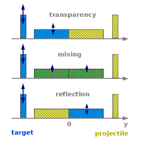
Figure 1: Sketch of the rapidity distributions of the baryon number or the particle production sources (horizontal rectangles) in nucleus-nucleus collisions resulting from the transparency, mixing and reflection models. The spectator nucleons are indicated by the vertical rectangles. In the collisions with the fixed number of projectile spectators only matter related to the target shows significant fluctuations (vertical arrows).

The spectra related to the projectile and the target can be easily distinguished in the figure because they are marked in color and hatching the same way as the initial projectile and target nuclei. In this paper we propose a method to mark the matter related to the projectile and the target in fluctuations (the MinF-method), which allows to test experimentally different scenarios of the collision process. Finally we apply the MinF-method to the NA49 experimental data on Pb+Pb collisions at 158$A$ GeV ($\sqrt{s_{NN}}$ = 17.2 GeV) maciek .

2. In each A+A collision only a part of all 2$A$ nucleons interact. These are called participant nucleons and they are denoted as $N_{P}^{proj}$ and $N_{P}^{targ}$ for the projectile and target nuclei, respectively. The nucleons which do not interact are called the projectile and target spectators, $N_{S}^{proj}=A-N_{P}^{proj}$ and $N_{S}^{targ}=A-N_{P}^{targ}$. The fluctuations in high energy A+A collisions are dominated by a trivial geometrical variation of the impact parameter. However, even for the fixed impact parameter the number of participants, $N_{P}\equiv N_{P}^{proj}+N_{P}^{targ}$, fluctuates from event to event. This is caused by the fluctuations of the initial states of the colliding nuclei and the probabilistic character of an interaction process. The fluctuations of $N_{P}$ usually form a large and uninteresting background. In order to minimize its contribution NA49 selected samples of collisions with fixed numbers of projectile participants. This selection is possible due to the measurement of $N_{S}^{proj}$ in each individual collision by use of a calorimeter which covers the projectile fragmentation domain. However, even in the samples with $N_{P}^{proj}=const$ the number of target participants fluctuates considerably. Hence, an asymmetry between projectile and target participants is introduced, i.e. $N_{P}^{proj}$ is constant, whereas $N_{P}^{targ}$ fluctuates. This difference is used in the MinF-method to distinguish between the final state flows related to the projectile and the target. Qualitatively, one expects large fluctuations of any extensive quantity (e.g. net baryon number and multiplicity of hadron production sources) in the domain related to the target and small fluctuations in the projectile region. When both flows are mixed intermediate fluctuations are predicted. The whole procedure is presented in a graphical form in Fig. 1. Clearly, the fluctuations measured in the target momentum hemisphere are larger than those measured in the projectile hemisphere in T-models. The opposite relation is predicted for R-models, whereas for M-models the fluctuations in the projectile and target hemispheres are the same.

This general qualitative idea is further on illustrated by quantitative calculations performed within several models ordered by an increasing complexity.

3. Let us begin with considering fluctuations of the net baryon number measured in different regions of the participant domain in collisions of two identical nuclei. These fluctuations are most closely related to the fluctuations of the number of participant nucleons because of the baryon number conservation. In the following the variance, $Var(x)\equiv\langle x^{2}\rangle-\langle x\rangle^{2}$, and the scaled variance, $\omega_{x}\equiv Var(x)/\langle x\rangle$, where $x$ stands for a given random variable and $\langle\cdots\rangle$ for event-by-event averaging, will be used to quantify fluctuations. We denote by $\omega_{P}^{targ}\equiv Var(N_{P}^{targ})/\langle N_{P}^{targ}\rangle$ the scaled variance of the number of target participants and by $\omega_{B}\equiv Var(B)/\langle B\rangle$ the scaled variance of the net baryon number, $B$. In each event we subtract the nucleon spectators when counting the number of baryons. The net baryon number, $B\equiv N_{B}-N_{\overline{B}}$, equals then the number of participants $N_{P}=N_{P}^{targ}+N_{P}^{proj}$. At fixed $N_{P}^{proj}$, the $N_{P}$ number fluctuates due to the fluctuations of $N_{P}^{targ}$. The distribution in $N_{P}^{targ}$ can be characterized by its mean value, $\langle N_{P}^{targ}\rangle\simeq N_{P}^{proj}$, and a scaled variance, $\omega_{P}^{targ}$. Thus, for the net baryon baryon number $B$ one finds,

$$\omega_{B}~{}=~{}\frac{Var(N_{P})}{\langle N_{P}\rangle}~{}\simeq~{}\frac{\langle\left(N_{P}^{targ}\right)^{2}\rangle~{}-~{}\langle N_{P}^{targ}\rangle^{2}}{2\langle N_{P}^{targ}\rangle}~{}=~{}\frac{1}{2}~{}\omega_{P}^{targ}~{},$$ (1)

for the fluctuations in the full phase space of participant nucleons. A factor $1/2$ in the right hand side of Eq. (1) appears because only a half of the total number of participants fluctuates. Let us introduce $\omega_{B}^{p}$ and $\omega_{B}^{t}$, where the superscripts $p$ and $t$ mark quantities measured in the projectile and target momentum hemispheres, respectively. By assumption, the mixing of the projectile and target participants is absent in T- and R-models. Therefore, in T-models, the net baryon number in the projectile hemisphere equals $N_{p}^{proj}$ and does not fluctuate, i.e. $\omega_{B}^{p}(T)=0$, whereas the net baryon number in the target hemisphere equals $N_{p}^{targ}$ and fluctuates with $\omega_{B}^{t}(T)=\omega_{P}^{targ}$. These relations are reversed in R-models.

We introduce now a random mixing of baryons between the projectile and target hemispheres. Let $\alpha$ be a probability for (projectile) target participant to be detected in the (target) projectile hemisphere. It is easy to show that:

$$\omega_{B}^{t}~{}=~{}(1~{}-~{}\alpha)^{2}~{}\omega_{P}^{targ}~{}+~{}2\alpha(1~{}-~{}\alpha)~{},~{}~{}~{}~{}\omega_{B}^{p}~{}=~{}\alpha^{2}~{}\omega_{P}^{targ}~{}+~{}2\alpha(1~{}-~{}\alpha)~{}.$$ (2)

A (complete) mixing of the projectile and target participants is assumed in M-models. Thus each participant nucleon with equal probability, $\alpha=1/2$, can be found either in the target or in the projectile hemispheres. In M-models the fluctuations in both hemispheres are identical. The limiting cases, $\alpha=0$ and $\alpha=1$ of Eq. (2) correspond to T- and R-models, respectively. In summary the scaled variances of the net baryon number fluctuations in the projectile, $\omega_{B}^{p}$, and target, $\omega_{B}^{t}$, hemispheres are:

$$\omega_{B}^{p}(T)~{}=~{}0~{},~{}~{}~{}~{}~{}~{}\omega_{B}^{t}(T)~{}=~{}\omega_{P}^{targ}~{},$$ (3)

$$\omega_{B}^{p}(M;~{}rr)~{}=~{}\omega_{B}^{t}(M;~{}rr)~{}=~{}\frac{1}{2}~{}+~{}~{}\frac{1}{4}~{}\omega_{P}^{targ}~{},$$ (4)

$$\omega_{B}^{p}(R)~{}=~{}\omega_{P}^{targ}~{},~{}~{}~{}~{}\omega_{B}^{t}(R)~{}=~{}0~{},$$ (5)

in the T- (3), M- (4) and R- (5) models of the baryon number flow. When deriving Eq. (4) we assumed that the baryons are distributed randomly in the rapidity space thus the abbreviation $rr$ in the left hand side of Eq. (4) stands for $random$ $rapidities$. This implies that even for a fixed number of $N_{P}^{targ}$, i.e. for $\omega_{P}^{targ}=0$, the baryon number in the projectile and target hemispheres fluctuates, $\omega_{B}^{p}(M;~{}rr)~{}=~{}\omega_{B}^{t}(M;~{}rr)~{}=~{}1/2$.

In a mixing model in which baryon rapidities do not fluctuate from collision to collision, but their positions are fixed (the $fixed$ $rapidity$, (fr), model) the scaled variances in the projectile and target hemispheres read:

$$\omega_{B}^{p}(M;~{}fr)~{}=~{}\omega_{B}^{t}(M;~{}fr)~{}=~{}\frac{1}{4}~{}\omega_{P}^{targ}~{}.$$ (6)

Note that the term $1/2$ of the right hand side of Eq. (4) is absent in (6).

Eventually, for an estimate of the magnitude of the expected fluctuations in different type of models we consider an example of Pb+Pb collisions at 158$A$ GeV. The scaled variance of the number of target participants at the fixed number of projectile participants (i.e. $\omega_{P}^{proj}=0$) can be calculated within the string-hadronic models. The corresponding results BHK obtained for the HSD hsd model are shown in Fig. 2, left.

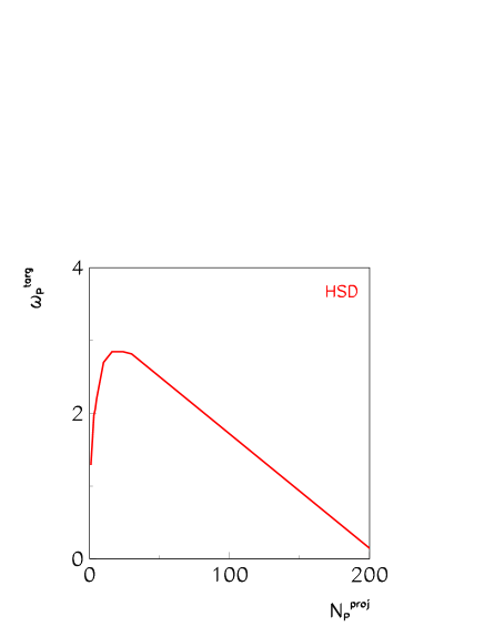
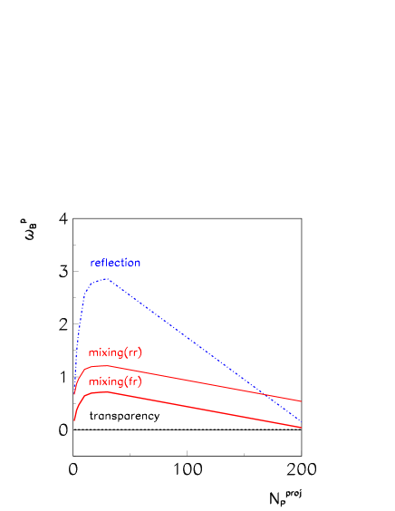
Figure 2: Left: The scaled variance $\omega_{P}^{targ}$ for the fluctuations of target participants $N_{P}^{targ}$ as a function of $N_{P}^{proj}$ calculated BHK within the HSD model. Right: The scaled variances $\omega_{B}^{p}$ versus $N_{P}^{proj}$ obtained within T- (dashed line) and R-models (dashed-dotted line), Eqs. (3, 5). The upper solid line shows predictions of the M-model with random rapidities of baryons (4) whereas the lower solid line corresponds to the M-models with fixed rapidities of baryons (6). For $\omega_{B}^{t}$ the predictions for T- and R-models should be exchanged and the lines for the M-models remain unchanged.

Using Eqs. (3-4) and the dependence of $\omega_{P}^{targ}$ on $N_{P}^{proj}$ calculated within the HSD model (Fig. 2 (left)), quantitative predictions concerning the baryon number fluctuations for different models can be obtained. The resulting dependencies of the scaled variance of the baryon number in the projectile hemisphere on $N_{P}^{proj}$ are shown in Fig. 2 (right). As expected large fluctuations are seen in R-models, intermediate in M-models and there are no fluctuations in T-models. In the M-model the scaled variance increases by 1/2 when baryon positions in rapidity are assumed to fluctuate.

4. The T-, M- and R-models for the baryonic flows give indeed very different predictions for $\omega_{B}^{p}$ and $\omega_{B}^{t}$ for the samples of events with fixed values of $N_{P}^{proj}$. However, they may be difficult to test experimentally as an identification of protons and a measurement of neutrons in a large acceptance in a single event is difficult. Measurements of charged particle multiplicity in a large acceptance can be performed using the existing detectors. In particular, the first results on multiplicity fluctuations of negatively charged hadrons, $N_{-}$, as a function of $N_{P}^{proj}$ were recently obtained by NA49 maciek for Pb+Pb collisions at 158$A$ GeV. Note that at the CERN SPS and lower energies negatively charged hadrons are predominantly (more than 90%) $\pi^{-}$ mesons. In the following we consider T-, M- and R- scenarios within several approaches to particle production in high energy nuclear collisions. We suppose that a part of the initial projectile and target energy, the inelastic energy, is converted into hadron sources. Further on, the numbers of projectile and target related sources are taken to be proportional to the number of projectile and target participant nucleons, respectively. The physical meaning of a particle source depends upon the model under consideration, examples are wounded nucleons (see wnm ; wnm1 ), strings and resonances (see hsd ; urqmd ), and volume cells of the expanding matter at the freeze-out in the hydrodynamical models. For the independent sources one finds regarding the scaled variance of $i$-th particle species (see e.g. source ):

$$\omega_{i}~{}=~{}\omega_{i}^{*}~{}+~{}\langle n_{i}^{*}\rangle~{}\Omega_{*}~{},$$ (7)

where $\omega_{i}^{*}$ denotes the scaled variance for $i$-th hadron species (e.g., $i$ may correspond to $h^{-}$) from a single source, $\langle n_{i}^{*}\rangle$ is the average multiplicity from a single source, and $\Omega_{*}$ is the scaled variance for the fluctuation of the number of sources. Assuming that the number of hadron sources is proportional to the number of participating nucleons, $N_{*}=const\cdot N_{P}$, one gets:

$$\langle n_{i}^{*}\rangle~{}\Omega_{*}~{}\equiv~{}\frac{\langle N_{i}\rangle}{\langle N_{*}\rangle}~{}\Omega_{*}~{}=~{}\frac{\langle N_{i}\rangle}{\langle N_{P}\rangle}~{}\omega_{P}~{}\equiv~{}\overline{n}_{i}~{}\omega_{P}~{},$$ (8)

where $\overline{n}_{i}$ is the average multiplicity of the $i$-th species per participating nucleon. Thus the scaled variance (7) of the particle number multiplicity in the full phase space is:

$$\omega_{i}~{}=~{}\omega_{i}^{*}~{}+~{}\overline{n}_{i}~{}\frac{1}{2}~{}\omega_{P}^{targ}~{}.$$ (9)

Consequently, the scaled variances of the $i$-th hadron multiplicity distribution in T-, M- and R-models read:

$$\omega_{i}^{p}(T)~{}=~{}\omega_{i}^{*}~{},~{}~{}~{}~{}\omega_{i}^{t}(T)~{}=~{}\omega_{i}^{*}~{}+~{}\overline{n}_{i}~{}\omega_{P}^{targ}~{},$$ (10)

$$\omega_{i}^{p}(M;~{}rr)~{}=~{}\omega_{i}^{t}(M;~{}rr)~{}=~{}\omega_{i}^{*}~{}+~{}\overline{n}_{i}~{}\left(~{}\frac{1}{2}~{}+~{}\frac{1}{4}~{}\omega_{P}^{targ}~{}\right)~{},$$ (11)

$$\omega_{i}^{p}(M;~{}fr)~{}=~{}\omega_{i}^{t}(M;~{}fr)~{}=~{}\omega_{i}^{*}~{}+~{}\overline{n}_{i}~{}\frac{1}{4}~{}\omega_{P}^{targ}~{},$$ (12)

$$\omega_{i}^{p}(R)~{}=~{}\omega_{i}^{*}~{}+~{}\overline{n}_{i}~{}\omega_{P}^{targ}~{},~{}~{}~{}~{}\omega_{i}^{t}(R)~{}=~{}\omega_{i}^{*}~{}.$$ (13)

Again two different versions of mixing with random rapidities (11) and fixed rapidities (12) of the source positions are possible. As an example of M-models with fixed rapidities of the sources let us consider a model which assumes a global equilibration of the matter at the early stage of collisions followed by a hydrodynamical expansion and freeze-out. In this case particle production sources can be identified with the volume cells of the expanding matter at the freeze-out. They can be treated as uncorrelated provided the effects of global energy-momentum conservation laws can be neglected. Due to assumed global equilibration of the projectile and target flows the fluctuations in the projectile and target hemispheres are identical. The model belongs to the class of M-models. In this model there is one to one correspondence between space-time positions and rapidities of the hydrodynamic cells. Thus, the source rapidities do not fluctuate and the scaled variances of hadrons in the projectile and target hemispheres have the form (12).

Note that Eqs. (10) and (13) are strictly valid provided that a source produces particles only in its hemisphere. Due of the finite width of the rapidity distribution resulting from the decay of a single source this condition is expected to be violated at least close to midrapidity. Thus, in order to be able to neglect the cross-talk of particles between the projectile and target hemispheres the width of the rapidity distribution of a single source, $\Delta y_{*}$, should be much smaller than the total width of the rapidity distribution.

Some comments concerning Eqs. (10-13) are appropriate. There is a general similarity of the expressions for produced particles and the corresponding expressions for baryons, Eqs. (3-6). There are, however, two important differences. A single source produces particles in a probabilistic way with an average multiplicity $\langle n_{i}^{*}\rangle$ and a scaled variance $\omega_{i}^{*}$. Consequently, it leads to an additional term, $\omega_{i}^{*}$, in all expressions for $\omega_{i}^{p,t}$, and an additional factor, $\overline{n}_{i}$, appears in terms related to the fluctuations of the number of sources. Following Eq. (8) the source number fluctuations can be substituted by $\omega_{P}^{targ}$, and an average multiplicity, $\langle n_{i}^{*}\rangle$, of a single source can be then transformed into an average multiplicity per participating nucleon, $\overline{n}_{i}$. The term, 1/2, in the r.h.s. of Eq. (11), as that in Eq. (4), is due to the random rapidity positions of the sources in M-models. In the hydrodynamical model particle production sources can be identified with the volume cells of the expanding matter at the freeze-out. The source rapidities do not fluctuate and Eq. (11) is transformed then into Eq. (12).

We turn now to a discussion of multiplicity fluctuations of negatively charged hadrons in Pb+Pb collisions at 158$A$ GeV. The value of $\langle N_{-}\rangle/\langle N_{P}\rangle\equiv\overline{n}_{-}\simeq 2$ was measured for the studied reactions peter . For simplicity we assume $\omega_{-}^{*}\simeq 1$, this is valid for the poissonian negatively charged particle multiplicity distribution from a single source. Note, in p+p interactions at SPS energies and in the limited acceptance of NA49 the measured distribution is in fact close to the Poisson one maciek . This gives:

$$\omega_{-}^{p}(T)~{}=~{}\omega_{-}^{t}(R)~{}\simeq~{}1~{},$$ (14)

$$\omega_{-}^{p}(M;~{}rr)~{}=~{}\omega_{-}^{t}(M;~{}rr)~{}\simeq~{}2~{}+~{}\frac{1}{2}~{}\omega_{P}^{targ}~{},$$ (15)

$$\omega_{-}^{p}(M;~{}fr)~{}=~{}\omega_{-}^{t}(M;~{}fr)~{}\simeq~{}1~{}+~{}\frac{1}{2}~{}\omega_{P}^{targ}$$ (16)

$$\omega_{-}^{t}(T)~{}=~{}\omega_{-}^{p}(R)~{}\simeq~{}1~{}+~{}2~{}\omega_{P}^{targ}~{}.$$ (17)

The dependence of $\omega_{-}^{p}$ on $N_{P}^{proj}$ from Eqs.(14-17) for T-, M- and R-models is presented in Fig. 3. .

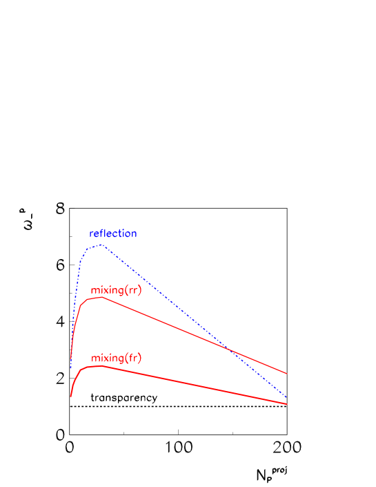
Figure 3: The dependence of the scaled variance of negatively charged particle multiplicity in Pb+Pb collisions at 158$A$ GeV on the number of projectile participants, $N_{P}^{proj}$, in the projectile hemisphere. The predictions for T- (14) and R- (17) models are shown by dashed and dashed-dotted lines, respectively. The upper solid line, mixing(rr), corresponds to the M-models with random rapidity positions of the sources (15). The lower solid line, denoted as mixing(fr), corresponds to the M-models with fixed rapidity positions of the sources (16). For the target hemisphere the lines of T- and R-models should be interchanged, whereas the lines of M-models remain unchanged. We take $\omega_{P}^{targ}$ from Fig. 2 (left) for all types of models.

5. In a recent analysis wnm1 of d+Au interactions at $\sqrt{s_{NN}}=200$ GeV Back:2004mr within the wounded nucleon model (WNM) wnm it was found that the wounded nucleon sources emit particles in a very broad rapidity interval which results in the mixing of particles from the target and projectile sources. In the following we consider predictions of this model with respect to multiplicity fluctuations.

The WNM assumes that $i$-th particle rapidity distribution in A+A collisions is presented as

$$\frac{dN_{i}}{dy}~{}=~{}N_{P}^{targ}~{}F_{i}^{t}(y)~{}+~{}N_{P}^{proj}~{}F_{i}^{p}(y)~{},$$ (18)

where $F_{i}^{t}(y)$ and $F_{i}^{p}(y)$ are the contributions from a single wounded nucleon (identified with a particle source) of the target and projectile, respectively. The model also requires

$$F_{i}^{p}(y)~{}=~{}F_{i}^{t}(-y)~{}$$ (19)

in the center of mass system of the collision. The mean number of particles in the rapidity interval $\Delta y$ for collisions with $N_{P}^{proj}$ and $N_{P}^{targ}$ is given by

$$N_{i}(\Delta y)~{}=~{}N_{P}^{targ}~{}\int_{\Delta y}dy~{}F_{i}^{t}(y)~{}+~{}N_{P}^{proj}~{}\int_{\Delta y}dy~{}F_{i}^{p}(y)~{}.$$ (20)

For interaction of identical heavy ions $\langle N_{P}^{targ}\rangle\simeq N_{P}^{proj}$, and then Eq. (20) yields:

$$\langle N_{i}(\Delta y)\rangle~{}=~{}N_{P}^{proj}~{}\int_{\Delta y}dy~{}\left[F_{i}^{t}(y)~{}+~{}F_{i}^{p}(y)\right]~{}.$$ (21)

Let us consider now fluctuations of $N_{i}(\Delta y)$ at a fixed $N_{P}^{proj}$. A contribution to the scaled variance of $N_{i}(\Delta y)$ (20) due to the fluctuations of $N_{P}^{targ}$ reads:

$$\frac{Var[N_{i}(\Delta y)]}{\langle N_{i}(\Delta y)\rangle}~{}=~{}\frac{\left[\int_{\Delta y}dy~{}F_{i}^{t}(y)\right]^{2}}{\int_{\Delta y}dy~{}\left[F_{i}^{t}(y)~{}+~{}F_{i}^{p}(y)\right]}~{}\omega_{P}^{targ}~{}\equiv~{}n_{i}^{t}(\Delta y)~{}\alpha^{t}_{i}(\Delta y)~{}\omega_{P}^{targ}~{},$$ (22)

where

$$n_{i}^{t}(\Delta y)~{}\equiv~{}\int_{\Delta y}dy~{}F_{i}^{t}(y)~{},~{}~{}~{}~{}\alpha^{t}_{i}(\Delta y)~{}\equiv~{}\frac{\int_{\Delta y}dy~{}F_{i}^{t}(y)}{\int_{\Delta y}dy~{}\left[F_{i}^{t}(y)~{}+~{}F_{i}^{p}(y)\right]}~{}.$$ (23)

As previously, for simplicity we assume that a single source emits particles according to the Poisson distribution, $\omega_{i}^{*}(\Delta y)=1$. This leads to a general expression on the scaled variance for a particle of $i$-th type:

$$\omega_{i}(\Delta y)~{}=~{}1~{}+n_{i}^{t}(\Delta y)~{}\alpha^{t}_{i}(\Delta y)~{}\omega_{P}^{targ}~{}.$$ (24)

The parameter $\alpha^{t}_{i}$ quantifies the amount of mixing of the projectile and target contributions and can vary between 0 and 1. For full acceptance, $\Delta y=[-Y_{max},Y_{max}]$, Eq. (24) transforms to Eq. (9).

The T-, M- and R- limits of the WNM can be formulated in terms of the distribution functions of the single nucleon,

$$F_{i}^{p}(y;T)~{}=~{}T_{i}(y)~{}\theta(y)~{},~{}~{}~{}~{}F_{i}^{t}(y;T)~{}=~{}T_{i}(-y)~{}\theta(-y)~{},$$ (25)

$$F_{i}^{p}(y;M)~{}=~{}F_{i}^{t}(y;M)~{}=~{}M_{i}(y)~{},$$ (26)

$$F_{i}^{p}(y;R)~{}=~{}R_{i}(-y)~{}\theta(-y)~{},~{}~{}~{}~{}F_{i}^{t}~{}=~{}R_{i}(y)~{}\theta(y)~{}.$$ (27)

The scaled variances in the projectile and target hemispheres, $\omega_{i}^{p}\equiv\omega_{i}(y\geq 0)$ and $\omega_{i}^{t}\equiv\omega_{i}(y\leq 0)$, can be found using Eq. (24). It follows that in T- and R-models, the $\omega_{i}^{p,t}$ coincide with those given by Eq. (10) and Eq. (13), respectively. For the M-models this gives the following result:

$$\omega_{i}^{p}(M;~{}WNM)~{}=~{}\omega_{i}^{t}(M;~{}WNM)~{}=~{}1~{}+~{}\overline{n}_{i}~{}\frac{1}{4}~{}\omega_{P}^{targ}~{},$$ (28)

which is identical to Eq. (12). In the WNM all projectile (target) sources are assumed to be identical and their positions are the same and fixed. Therefore, similar to the hydrodynamical model, the term, 1/2, in the r.h.s. of Eq. (11) is absent in Eq. (28). This is the M-model with the fixed rapidity positions of the sources. The mixing in the considered version of WNM results from a broad distribution of particles produced by a single source. A complete mixing in the WNM means according to Eq. (26) that projectile and target source functions become identical.

6. Let us consider fluctuations in limited phase-space domains in which only fractions, $q^{p,t}$, of all particles in the projectile or target hemispheres are accepted. Then the scaled variances in the acceptance, $\omega^{p}_{acc}$ and $\omega^{t}_{acc}$, will be different from the $\omega^{p}$ and $\omega^{t}$. We start with the scaled variances $\omega_{B}^{p}$ and $\omega_{B}^{t}$ of the net baryon number fluctuations. Assuming that inside the projectile and target hemispheres the baryon rapidities are not correlated one gets (see e.g.,source ; ce1 ):

$$\omega^{p,t}_{B,acc}~{}=~{}1~{}-~{}q^{p,t}~{}+~{}q^{p,t}\cdot\omega_{B}^{p,t}~{}.$$ (29)

It can be shown that the scaled variance of the produced particles in the limited momentum acceptance within the M-model with fixed source rapidities (12) reads:

$$\omega_{i,acc}(M,~{}fr)=1+\frac{1}{2}\frac{\langle N_{i}\rangle_{acc}}{\langle N_{P}\rangle}\omega_{P}^{targ}~{},$$ (30)

where $\langle N_{i}\rangle_{acc}$ is a mean multiplicity of a particle of $i$-th type in the acceptance. The formula above assumes that the produced particles are uncorrelated in the momentum space, i.e. it neglects effects of motional conservation laws and resonance decays. The scaled variance in a limited rapidity acceptance, $\Delta y$, within WNM can be directly obtained from Eq. (24). It coincides with that of Eq. (30).

Let us consider now as an example the NA49 acceptance, which is located in the projectile hemisphere about one and half rapidity units from mid-rapidity, $\Delta y=[1.1;~{}2.6]$ in the c.m.s. The acceptance probability was measured to be $q^{p}\simeq 0.4$ maciek ; kasia (i.e. about 40% of negatively charged particles in the projectile hemisphere are accepted). In the limiting case of the fixed rapidities of the sources, this is assumed to be valid for both the hydrodynamical and WN models, one finds:

$$\omega_{-,acc}^{p}(T)~{}\simeq~{}1,$$ (31)

$$\omega_{-,acc}^{p}(M;~{}fr)~{}\simeq~{}1~{}+~{}0.2~{}\omega_{P}^{targ}~{},$$ (32)

$$\omega_{-,acc}^{p}(R;~{}fr)~{}\simeq~{}1~{}+~{}0.8~{}\omega_{P}^{targ}~{}.$$ (33)

The relations, $n_{-}^{t}(\Delta y;T)=0;~{}~{}n_{-}^{t}(\Delta y;M)~{}=~{}0.5~{}q^{p}~{}\overline{n}_{-};~{}~{}n_{-}^{t}(\Delta y;R)~{}=~{}q^{p}~{}\overline{n}_{-}$, with $q^{p}~{}\simeq~{}0.4$ and $\overline{n}_{-}~{}\simeq~{}2$ have been used in Eqs. (31-33). Note that in the limit $q^{p}\rightarrow 0$ one finds $\omega_{-,acc}^{p}\simeq 1$ for all type of models.

The predictions given by Eqs. (31-33) are shown in Fig. 4. One may be surprised that different models lead to the same results for most central collisions. This is because $\omega_{P}^{targ}$ goes to zero at $N_{P}^{proj}\simeq A$, as it follows from Fig. 2 (left). The predictions of the T-, M- and R-models differ because of their different response on the $N_{P}^{targ}$ fluctuations. These fluctuations become small in the most central events. Therefore, the best way to study the mixing-transparency effects is the analysis of the centrality dependence of the particle number fluctuations in the projectile and target hemispheres.

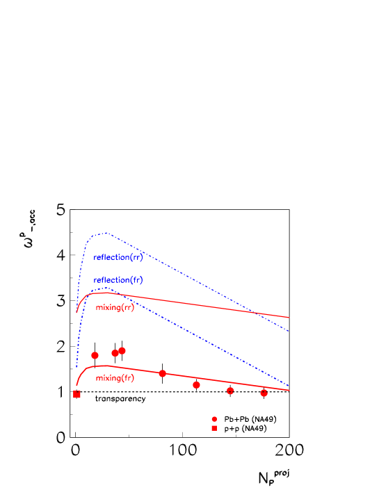
Figure 4: The dependence of the scaled variance of negatively charged particle multiplicity in Pb+Pb collisions at 158$A$ GeV on the number of projectile participants, $N_{P}^{proj}$, in the NA49 acceptance located in the projectile hemisphere. The Pb+Pb data maciek are indicated by filled circles. For a comparison the result for p+p interactions at 158 GeV maciek ; kasia is shown by the filled square. The displayed errors correspond to the sum of systematic and statistical uncertainties. The dashed line shows a dependence predicted within T-models (Eqs. (31) and (34)), the solid lines correspond to the mixing(fr) models (lower line, Eq. (32)), and the mixing(rr) models (upper line, Eq. (35)). The lower dashed-dotted line corresponds to the reflection(fr) models (33)), whereas the reflection(rr) models (36) are indicated by the upper dashed-dotted line.

We now discuss an effect of a limited acceptance for the approaches with randomly fluctuating source rapidities. In this case the scaled variances in the projectile and target hemispheres are given by Eqs. (10-13), provided a width of a rapidity spectrum of particles emitted from a single source is narrow. In a general case, when a rapidity width of the source particles and an acceptance window are comparable in size, it is difficult to make analytical estimates. The problem can be solved in the limit of very narrow sources (a source width, $\Delta y_{*}$, is much smaller than the experimental acceptance interval, $\Delta y$). The hadrons created by ”narrow” sources have correlated rapidities, but Eq. (29) can be used for the scaled variances of the number of sources assuming that the source rapidities in the projectile hemisphere are not correlated. In this case our Eqs. (10-13) yield:

$$\omega_{-,acc}^{p}(T;~{}rr)~{}\simeq~{}1,$$ (34)

$$\omega_{-,acc}^{p}(M;~{}rr)~{}\simeq~{}1~{}+~{}\overline{n}_{-}~{}\left[1~{}-~{}q^{t}~{}+~{}q^{t}\cdot\left(\frac{1}{2}~{}+~{}\frac{1}{4}~{}\omega_{P}^{targ}\right)\right]~{}\simeq~{}2.6~{}+~{}0.2~{}\omega_{P}^{targ}~{},$$ (35)

$$\omega_{-,acc}^{p}(R;~{}rr)~{}\simeq~{}1~{}+~{}\overline{n}_{-}~{}\left[1~{}-~{}q^{t}~{}+~{}q^{t}\cdot~{}\omega_{P}^{targ}\right]~{}\simeq~{}2.2~{}+~{}0.8~{}\omega_{P}^{targ}~{}.$$ (36)

As before, we use $q^{p}~{}\simeq~{}0.4$ and $\overline{n}_{-}~{}\simeq~{}2$ in Eqs. (34-36). The corresponding curves are plotted in Fig. 4.

The experimental points for Pb+Pb collisions at 158$A$ GeV clearly exclude transparency and reflection approaches discussed here. The mixing model with random fluctuations of a source rapidity and a narrow width also strongly disagree with the data. A reasonable agreement is observed only for the mixing-hydrodynamical and WNM models. We remind that a large degree of mixing was found previously in the analysis of the pseudo-rapidity spectra of charged hadrons produced in d+Au interactions at $\sqrt{s_{NN}}=$ 200 GeV Back:2004mr within WNM wnm1 .

Note however that the WNM model, used here as a simple example to illustrate the MinF method, can not reproduce many observables connected to collective behavior of matter created in high energy nuclear collisions, like radial and anisotropic flows and the strangeness enhancement. On the other hand, these effects are at least qualitatively described by statistical and hydrodynamical approaches.

7. At the end several comments are appropriate. We considered three limiting behaviors of nuclear flows: transparency, mixing and reflection. In general, all intermediate cases are possible and they can be characterized by an additional parameter. Eq. (2) introduces a mixing parameter $\alpha$ for the net baryon number with limiting cases $\alpha(T)=0$, $\alpha(M)=1/2$, and $\alpha(R)=1$ for T-, M- and R-models, respectively. Within WNM a parameter, $\alpha_{i}^{t}(\Delta y)$ (23), defined for each particle species, $i$, and for each rapidity interval, $\Delta y$, was suggested. The limiting cases are again: $\alpha_{i}^{t}(\Delta y;T)=0,~{}\alpha_{i}^{t}(\Delta y;M)=0.5$, and $\alpha_{i}^{t}(\Delta y;R)=1$. The values of the mixing parameter can be extracted by fitting the experimental data.

The fluctuations of the participant number lead to the fluctuations of the center of mass rapidity ($\Delta y\simeq-1/2\log(N_{P}^{targ}/N_{P}^{proj})$. This alone may result in additional multiplicity fluctuations. We estimated that for the NA49 data discussed above the corresponding increase of the scaled variance is smaller than 5%.

The MinF-method can be used independently of the degrees of freedom relevant at an early stage of collisions (e.g. hadrons at a low collision energy or quark and gluons at a high energy). This is because the concepts of the spectators and the participants as well as hadron multiplicity fluctuations are valid at all relativistic energies and for all collision scenarios. In the case of collisions of non-identical nuclei (different baryon numbers and/or electric charge to baryon ratios) one can trace flows of the conserved charges by looking at their inclusive final state distributions (see e.g. fopi ). An interesting information can be extracted from collisions of two nuclei with different atomic numbers (see wnm1 ).

In the case of identical nuclei only the MinF method can be used. It gives a unique possibility to investigate the flows of both the net baryon number and particle production sources.

8. In summary, a method which allows to find out what happens with the initial flows in high energy nucleus-nucleus collisions was proposed. First, the projectile and target initial flows are marked in fluctuations (the MinF-method) in the number of colliding nucleons. This can be achieved by a selection of collisions with a fixed number of projectile participants but a fluctuating number of target participants. This case is considered in details in the present study. Other selections are also possible. Secondly, the projectile and target related matter in the final state of collisions are distinguished by an analysis of fluctuations of extensive quantities. We apply this method to the NA49 data on multiplicity fluctuations of negatively charged hadrons produced in Pb+Pb collisions at 158$A$ GeV maciek . The results are consistent with the model which assumes a significant degree of mixing of the projectile and target flows at the early stage of collisions followed by the hydrodynamical expansion and freeze-out.

We would like to thank V.V. Begun, A. Bialas, E.L.  Bratkovskaya, S. Haussler, Yu.B. Ivanov, V.P.  Konchakovski, B. Lungwitz, I.N. Mishustin, St. Mrówczyński, M. Rybczyński, H. Stöcker, and Z.  Włodarczyk for numerous discussions. Moreover, we are grateful to Marysia Gaździcka for help in the preparation of the manuscript. The work was supported in part by US Civilian Research and Development Foundation (CRDF) Cooperative Grants Program, Project Agreement UKP1-2613-KV-04 and Virtual Institute on Strongly Interacting Matter (VI-146) of Helmholtz Association, Germany.

References

- (1) For a recent summary see: Proceedings of the 17th International Conference on Ultra-Relativistic Nucleus-Nucleus Collisions, Oakland, California, USA, 11-17 January 2004, Eds. H. G. Ritter and X.-N. Wang, J. Phys. G 30, S663 (2004)
- (2) S. V. Afanasiev et al. [The NA49 Collaboration], Phys. Rev. C 66, 054902 (2002). M. Gazdzicki et al. [NA49 Collaboration], J. Phys. G 30, S701 (2004).
- (3) M. Gazdzicki and M. I. Gorenstein, Acta Phys. Polon. B 30, 2705 (1999).
- (4) I. Arsene et al. [BRAHMS Collaboration], Nucl. Phys. A 757, 1 (2005), B. B. Back et al., Nucl. Phys. A 757, 28 (2005), J. Adams et al. [STAR Collaboration], Nucl. Phys. A 757, 102 (2005), K. Adcox et al. [PHENIX Collaboration], Nucl. Phys. A 757, 184 (2005).
- (5) W. Cassing, E.L. Bratkovskaya and S. Juchem, Nucl. Phys. A674, 249 (2000).
- (6) S. A. Bass et al. (UrQMD Collab.), Prog. Part. Nucl. Phys. 41, 255 (1998).
- (7) Z. W. Lin, C. M. Ko, B. A. Li, B. Zhang and S. Pal, arXiv:nucl-th/0411110.
- (8) E. Fermi, Prog. Theor. Phys. 5, 570 (1950).
- (9) L. D. Landau, Izv. Akad. Nauk SSSR, Ser. Fiz. 17, 51 (1953).
- (10) U. Katscher, D. H. Rischke, J. A. Maruhn, W. Greiner, I. N. Mishustin and L. M. Satarov, Z. Phys. A 346, 209 (1993), Yu. B. Ivanov, V.N. Russkikh and V. D. Toneev, Phys. Rev. C 73, 044904 (2006).
- (11) M. Rybczynski et al. [NA49 Collaboration], J. Phys. Conf. Ser. 5, 74 (2005).
- (12) V. P. Konchakovski et al., Phys. Rev. C 73, 034902 (2006); arXiv:nucl-th/0511083.
- (13) A. Bialas and W. Czyz, Acta Phys. Polon. B 36, 905 (2005).
- (14) B. B. Back et al. [PHOBOS Collaboration], Phys. Rev. C 72, 031901 (2005) [arXiv:nucl-ex/0409021].
- (15) A. Bialas, M. Bleszynski and W. Czyz, Nucl. Phys. B 111, 461 (1976).
- (16) H. Heiselberg, Phys. Rep. 351, 161 (2001).
- (17) T. Anticic et al. [NA49 Collaboration], Phys. Rev. C 70, 034902 (2004) [arXiv:hep-ex/0311009].
- (18) P. Dinkelaker [NA49 Collaboration], J. Phys. G 31 (2005) S1131.
- (19) V. V. Begun, M. Gazdzicki, M. I. Gorenstein and O. S. Zozulya, Phys. Rev. C 70, 034901 (2004).
- (20) B. Hong et al. [FOPI Collaboration], Phys. Rev. C 66, 034901 (2002).