ON THE NONPERTURBATIVE FOUNDATIONS OF THE DIPOLE PICTURE

Starting from a genuinely nonperturbative formulation of photon-proton scattering we discuss which approximations and assumptions are required to obtain the dipole picture of high energy scattering.

1 Introduction

In the last few years the dipole picture of deep inelastic photon-hadron scattering $\!{}^{{\bf?},{\bf?}}$ has been widely used as a framework for interpreting HERA data, in particular in view of potential saturation effects at high energies. In the dipole picture the photon splits into a quark-antiquark pair – a colour dipole – which subsequently scatters off the proton. Accordingly, the cross section for transversely ($T$) or longitudinally ($L$) polarised photons is given by

$$\sigma_{T,L}(x,Q^{2})=\sum_{q}\int d^{2}R_{T}\int_{0}^{1}d\alpha\left|\psi^{(q)}_{T,L}(\alpha,\mathbf{R}_{T},Q)\right|^{2}\sigma^{(q)}_{\rm red}(R_{T}^{2},s)\,,$$ (1)

where $\sqrt{s}$ is the energy and $x=Q^{2}/s$ is the Bjorken scaling variable with the photon virtuality $Q^{2}$. The photon wave function $\psi_{T,L}^{(q)}$ describes in leading order in perturbation theory the splitting of the photon into a quark and an antiquark of flavour $q$ with relative separation $\mathbf{R}_{T}$ in transverse space, carrying the longitudinal momentum fractions $\alpha$ and $1-\alpha$, respectively. The reduced cross section $\sigma_{\rm red}$ describes the dipole-proton scattering. Note that according to Eq. (1) the energy dependence of the cross section is contained only in $\sigma_{\rm red}$. In practical applications of the dipole picture one fits the data by a suitable choice of the reduced cross section $\sigma_{\rm red}$. A prominent example is the Golec-Biernat-Wüsthoff model $\!{}^{{\bf?}}$ for $\sigma_{\rm red}$ which incorporates saturation effects.

The dipole picture in the form described above is perturbatively motivated and is thus expected to be valid for large photon virtualities and small values of $x$. Since at HERA small $x$ is correlated with smaller virtualities, however, the actual interest is mostly concentrated on the region of medium (and sometimes even small) virtualities where potential saturation effects could be observed. It is therefore an important question whether the simple dipole picture as given by the above formula is complete, or whether there are contributions to photon-proton scattering that cannot be accommodated by Eq. (1). More generally, it is crucial to understand which assumptions and approximations are required in order to obtain the dipole picture starting from a completely nonperturbative framework, and which potential corrections consequently need to be considered.

In the following we report in condensed form on a recent study $\!{}^{{\bf?},{\bf?}}$ in which we address these questions. For a detailed presentation we refer the interested reader to these references.

2 Functional Methods for the Compton Amplitude

We consider the Compton amplitude for real or virtual photons,

$$\gamma^{(*)}(q)+p(p)\,\,\,\longrightarrow\,\,\,\gamma^{(*)}(q^{\prime})+p(p^{\prime})\,,$$ (2)

and assume that $q^{2}=-Q^{2}\leq 0$ and $q^{\prime\,2}=-Q^{\prime\,2}\leq 0$. The matrix element for this process is

$$\mathcal{M}^{\mu\nu}_{s^{\prime}s}(p^{\prime},p,q)=\frac{i}{2\pi m_{p}}\int d^{4}x~{}e^{-iqx}\langle p(p^{\prime},s^{\prime})|\mbox{T}^{*}J^{\mu}(0)J^{\nu}(x)|p(p,s)\rangle\,,$$ (3)

with the proton helicities $s,s^{\prime}$ and with the electromagnetic current $J^{\lambda}(x)=\sum_{q}\bar{q}(x)Q_{q}\gamma^{\lambda}q(x)$, where $q=u,d,\dots$ are the quark field operators and $Q_{q}$ are the quark charges in units of the proton charge. According to the LSZ formula we can write this matrix element as

$$\mathcal{M}^{\mu\nu}_{s^{\prime}s}(p^{\prime},p,q) = -\frac{i}{2\pi m_{p}Z_{p}}\int d^{4}y^{\prime}~{}d^{4}y~{}d^{4}x\,e^{ip^{\prime}y^{\prime}}\bar{u}_{s^{\prime}}(p^{\prime})(-i\!\stackrel{{\scriptstyle\rightarrow}}{{\not\!\partial}}_{y^{\prime}}+m_{p})$$ (4)

$${}\left\langle\psi_{p}(y^{\prime})J^{\mu}(0)e^{-iqx}J^{\nu}(x)\overline{\psi}_{p}(y)\right\rangle_{G,q,\bar{q}}\,(i\!\stackrel{{\scriptstyle\leftarrow}}{{\not\!\partial}}_{y}+m_{p})u_{s}(p)e^{-ipy}\,,$$

where $\psi_{p}(x)=\Gamma_{\alpha\beta\gamma}u_{\alpha}(x)u_{\beta}(x)d_{\gamma}(x)$ is an interpolating field operator for the proton. $\langle\dots\rangle_{G,q,\bar{q}}$ indicates a functional integral average over all gluon and quark field configurations with the weight $\exp[i\int d^{4}x\,{\cal L}_{\rm QCD}]$. Inserting the electromagnetic currents and performing the Gaussian integral over quark fields yields a decomposition of the amplitude as a sum over all possible contractions of quark field operators, that is a classification of contributions according to their quark line skeleton. Fig. 1 shows the diagrammatic representation of these classes.

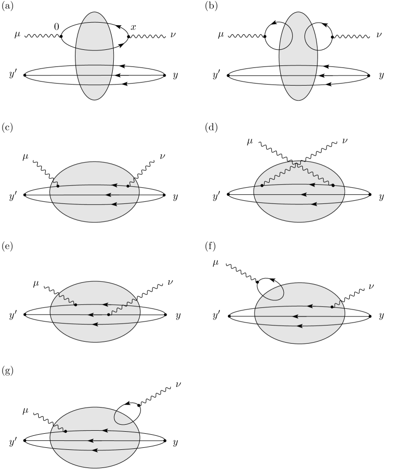
Figure 1: Classification of contributions to the Compton amplitude according to their quark line skeleton

The oriented lines represent nonperturbative quark propagators in the background of a gluon potential, indicated by the shaded blob, and we have to average over all possible gluon field configurations.

A closer inspection of these diagram classes reveals that only the contributions from the classes (a) and (b) are leading at high energies, whereas the other classes correspond to fermion exchanges in the $t$-channel and are suppressed by powers of the energy. We will therefore not consider the latter any further. The perturbative expansion of the contributions of class (b) starts at higher order than that of class (a). At large photon virtualities class (b) is therefore suppressed with respect to class (a) by powers of $\alpha_{s}$. Moreover, it turns out that only class (a) gives rise to the usual dipole picture. Hence we will assume in the following:

• The contribution of class (b) can be neglected.

At low photon virtualities, however, the suppression of class (b) is lifted and there will be a correction to the dipole picture coming from this class.

The contribution ${\cal M}^{(a)}$ to the Compton amplitude coming from the class (a) of Fig. (1) can be expressed as

$$\mathcal{M}^{(a)\mu\nu}_{s^{\prime}s}(p^{\prime},p,q) = -\frac{i}{2\pi m_{p}Z_{p}}\int d^{4}y^{\prime}~{}d^{4}y\,e^{ip^{\prime}y^{\prime}}\bar{u}_{s^{\prime}}(p^{\prime})(-i\!\stackrel{{\scriptstyle\rightarrow}}{{\not\!\partial}}_{y^{\prime}}+m_{p})$$ (7)

$${}\sum_{q}Q^{2}_{q}\Big{\langle}\mathop{\vbox{\halign{#\cr\kern 1.72218pt\cr$\hbox{$\hskip 3.25696pt\vrule height=7.31946pt,width=0.29999pt,depth=-0.11153pt\kern-0.29999pt\vrule height=7.31946pt,width=23.15385pt,depth=-7.01947pt\kern-0.29999pt\vrule height=7.31946pt,width=0.29999pt,depth=1.15515pt$\hss}$\crcr\kern 1.72218pt\nointerlineskip\cr\hbox{$\displaystyle{}{\psi}{{}_{p}(y^{\prime})}{\overline{\psi}}_{p}(y)$}\crcr}}}\limits A^{(q)\mu\nu}(q)\Big{\rangle}_{G}\,(i\!\stackrel{{\scriptstyle\leftarrow}}{{\not\!\partial}}_{y}+m_{p})u_{s}(p)e^{-ipy}\,,$$

where

$$A^{(q)\mu\nu}(q)=\int d^{4}x\,\mathrm{Tr}\left[\gamma^{\mu}S^{(q)}_{F}(0,x;G)e^{-iqx}\gamma^{\nu}S^{(q)}_{F}(x,0;G)\right]\,,$$ (8)

and the $S_{F}^{(q)}$ are nonperturbative quark propagators in the gluon potential $G$. Here we insert next to the photon vertex (that is next to $\gamma^{\nu}$) factors of $1$ in the form

$$(i\!\stackrel{{\scriptstyle\rightarrow}}{{\not\!\partial}}_{x}-m_{q})S_{F}^{(q,0)}(x,y)=-\delta^{(4)}(x-y)\,,$$ (9)

which contains a free quark propagator $S_{F}^{(q,0)}$ of (still arbitrary) mass $m_{q}$. Next we use the spin sum decompositions $\not\!k+m_{q}=\sum_{r}u_{r}(k)\bar{u}(k)$ and $\not\!k-m_{q}=\sum_{r}v_{r}(k)\bar{v}(k)$ in the spectral representation for the free quark propagator,

$$S^{(q,0)}_{F}(x,y) = -\frac{1}{2\pi}\int^{\infty}_{-\infty}\frac{d\omega}{\omega+i\epsilon}\int\frac{d^{3}k}{(2\pi)^{3}2k^{0}}$$ (10)

$${}\sum_{r}\left\{e^{-ik_{\omega}x}u_{r}(k)\bar{u}_{r}(k)e^{ik_{\omega}y}-e^{ik_{\omega}x}v_{r}(k)\bar{v}_{r}(k)e^{-ik_{\omega}y}\right\}$$

with $k_{\omega}=(k^{0}+\omega,\mathbf{k})$, and insert this in $A^{(q)\mu\nu}$ of (8) and further in (7) which finally leads us to an expression of $\mathcal{M}^{(a)\mu\nu}$ as a sum of four terms,

$$\mathcal{M}^{(a)\mu\nu}_{s^{\prime}s}(p^{\prime},p,q)=\sum^{4}_{j=1}\mathcal{M}^{(a,j)\mu\nu}_{s^{\prime}s}(p^{\prime},p,q)\,,$$ (11)

the first of which reads

$$\mathcal{M}^{(a,1)\mu\nu}_{s^{\prime}s}(p^{\prime},p,q)\! = \!\frac{1}{2\pi}\sum_{q}Q^{2}_{q}\int\frac{d\omega}{\omega+i\epsilon}\int\frac{d^{3}k}{(2\pi)^{3}2k^{0}}\,(q^{0}-k^{0}-k^{{\prime}0}-\omega+i\epsilon)^{-1}\,(2k^{{\prime}0})^{-1}$$

$${}\sum_{r^{\prime},r}\langle\gamma(q^{\prime},\mu),p(p^{\prime},s^{\prime})|\mathcal{T}^{(a)}|\bar{q}(k^{{\prime}}_{\omega},r^{\prime}),q(k_{\omega},r),p(p,s)\rangle\,\bar{u}_{r}(k)Z_{q}\gamma^{\nu}v_{r^{\prime}}(k^{{\prime}})\,,$$

where $k^{\prime}=(\sqrt{m_{q}^{2}+(\mathbf{q}-\mathbf{k})^{2}},\mathbf{q}-\mathbf{k})$ and $k^{\prime}_{\omega}=((q-k)^{0}-\omega,\mathbf{q}-\mathbf{k})$. The other three terms contain the other combinations of spinors, $\bar{u}\gamma^{\nu}u$, $\bar{v}\gamma^{\nu}u$, and $\bar{v}\gamma^{\nu}v$. In those terms the spinors have different momentum arguments, the matrix elements of ${\cal T}^{(a)}$ are crossed, and there appear different energy denominators. What we have done here is basically to cut open the trace in (8). Note that the quarks entering the matrix element are off the energy shell. The four terms have an interpretation which is reminiscent of old-fashioned perturbation theory $\!{}^{{\bf?}}$, but we stress that our procedure has been completely nonperturbative so far. It turns out that only in the term in (2) a quark and an antiquark come together with the proton in the incoming state of the matrix element, and thus only this term can give rise to the dipole picture.

In (2) we have introduced the renormalisation factor $Z_{q}$ such that the ${\cal T}^{(a)}$-matrix element becomes a properly renormalised $T$-matrix element if quarks are assumed to have a mass shell. At the same time the factor $Z_{q}$ is necessary for the proper renormalisation of the photon-quark-antiquark vertex which has been widely discussed in the context of overlapping divergences in QED. It can be written here in terms of the renormalised vertex function $\Gamma^{(q)}$ and a rescattering term,

$$Z_{q}\gamma^{\nu}=\Gamma^{(q)\nu}(l,l^{\prime})+\sum_{q^{\prime}}\int K^{(q,q^{\prime})}S^{(q^{\prime})}_{F}\Gamma^{(q^{\prime})\nu}S^{(q^{\prime})}_{F}\,.$$ (13)

After inserting this back into (2) we obtain two terms which are illustrated in Fig. 2.

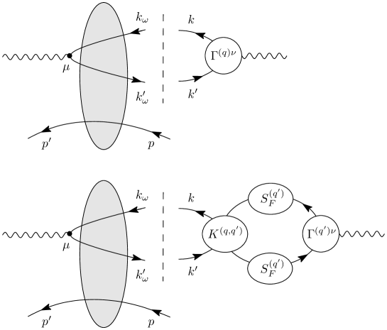
Figure 2: The two terms for the amplitude $\mathcal{M}^{(a,1)}$ after applying (13). The arrows on the lines indicate the interpretation as particle or antiparticle. The orientation of the momentum assignment to the lines is from right to left, irrespective of the arrows on the lines.

The dashed vertical line stands for the integration over $\omega$ and $d^{3}k$ in (2). The quarks to the right of that line are on-shell, while those to the left are off the energy shell.

The perturbative expansion of the rescattering term starts at higher order in $\alpha_{s}$ than the vertex term. At high $Q^{2}$ we can make the following assumption necessary for obtaining the dipole formula (1):

• The rescattering term in (13) is dropped and the vertex function $\Gamma^{(q)\nu}$ is taken at leading order, that is $\Gamma^{(q)\nu}=\gamma^{\nu}$.

At lower photon virtualities we expect a correction to the dipole picture coming from the rescattering term.

3 High Energy Limit

In the high energy limit, $|\mathbf{q}|\to\infty$, we find that $\Delta E=k^{0}+k^{\prime 0}-q^{0}\,\to\,0$. It turns out that of the four terms in (11) only the term $\mathcal{M}^{(a,1)\mu\nu}$ exhibits a pinch singularity in the $\omega$-integration in this limit and hence gives the leading contribution which we can obtain in the form

$$\mathcal{M}^{(a,1)\mu\nu}_{s^{\prime}s}(p^{\prime},p,q) = i\sum_{q}Q^{2}_{q}\int\frac{d^{3}k}{(2\pi)^{3}2k^{0}2k^{\prime 0}}\,(\Delta E)^{-1}\,\theta\left(\bar{Q}^{2}-\tilde{m}^{2}(\alpha,\mathbf{k}_{T})\right)$$

$${}\sum_{r^{\prime},r}\,\langle\gamma(q^{\prime},\mu),p(p^{\prime},s^{\prime})|\mathcal{T}^{(a)}|\bar{q}(k^{\prime},r^{\prime}),q(k,r),p(p,s)\rangle\,\bar{u}_{r}(k)\gamma^{\nu}v_{r^{\prime}}(k^{\prime})\,.$$

We do not have enough space here to discuss in detail the $\theta$-function in this expression. We would only like to point out that it emerges naturally from the discussion of the pinch singularity and that it later on provides a regularisation of any singularity arising in the photon wave function of small distances.

Contracting (3) with the polarisation vectors for transversely or longitudinally polarised photons leads to the well-known expressions for the corresponding photon wave functions. Since (3) is not separately gauge invariant, however, the longitudinal polarisation vector needs to be chosen such that its components remain finite in the high energy limit. Other choices lead to incorrect (and in fact arbitrary) results for the longitudinal photon wave function.

Some further steps are required to finally obtain the dipole formula (1). Obviously, we need to apply the procedure described above also to the outgoing photon. In order to be able to interpret the matrix elements in our formulae above (for example that of ${\cal T}^{(a)}$ in (2)) as actual $T$-matrix elements we have to make the following assumption:

• Quarks have a mass shell $m_{q}$ and can be treated as asymptotic states.

With this assumption we can then relate the $T$-matrix element to the reduced cross section and can be sure that the latter is non-negative. Assumption (iii) also allows us to define properly normalised dipole states which can then be interpreted as hadronic initial and final states.

Finally, two further assumptions are needed in order to find the factorised form of Eq. (1):

• At high energy the $T$-matrix for a dipole and a proton both in the incoming and in the outgoing state is diagonal in flavour, in the momentum fraction $\alpha$ carried by the quark as well as in the transverse separation $\mathbf{R}_{T}$ of the quark and antiquark in the dipole.

• The reduced matrix element $\sigma^{(q)}_{\rm red}$ depends only on $R_{T}^{2}$ and $s$, but is independent of the longitudinal momentum fraction $\alpha$.

Clearly, there will be corrections to both of these assumptions from various sources. An example are the diagrams coming from the class (b) in Fig. (1), which will become relevant at lower photon virtualities. It is quite obvious that these diagrams do in general not fulfil assumption (iv). Corrections are also expected from subleading diagrams in $\alpha_{s}$ in general.

With the assumptions and approximations (i)-(v) above we finally obtain the dipole picture and the photon-proton cross section at high energy in the form (1).

4 Summary

Starting from a completely nonperturbative formulation of photon-proton scattering we have identified the assumptions and approximations (i)-(v) that are needed in order to obtain the dipole picture at high energies. At the same time we have found corrections to the dipole picture which can become large at small photon virtualities. We consider it an important task for the future to investigate in detail the validity of the assumptions, the accuracy of the approximations, and the size of the corrections. In our opinion these issues should be addressed in order to put the results obtained in the framework of the dipole picture on solid ground.

The framework developed here should be suitable for studying the effects caused by the non-existence of a mass-shell for quarks, and for using nonperturbative quark propagators, obtained for example from Dyson-Schwinger equations or from lattice simulations, in phenomenology.

References

References

- [1] N. N. Nikolaev and B. G. Zakharov, Z. Phys. C 49 (1991) 607.
- [2] A. H. Mueller, Nucl. Phys. B 415 (1994) 373.
- [3] K. Golec-Biernat and M. Wüsthoff, Phys. Rev. D 59 (1999) 014017 [arXiv:hep-ph/9807513].
- [4] C. Ewerz and O. Nachtmann, arXiv:hep-ph/0404254.
- [5] C. Ewerz and O. Nachtmann, to be published