KEK-TH-1046

TUM-HEP-607/05

SISSA-81/2005/EP

Effective theoretical approach of Gauge-Higgs unification model and its phenomenological applications

Naoyuki Haba^(a,b), , Shigeki Matsumoto^(c), , Nobuchika Okada^(c,d), , and Toshifumi Yamashita^(c,e),
(a)Institute of Theoretical Physics, University of Tokushima, 770-8502, Japan
^(b)Physik-Department, Technische Universitat Munchen, James-Franck-Strasse, D-85748 Garching, Germany
^(c)Theory Group, KEK, Oho 1-1 Tsukuba, 305-0801, Japan
^(d)The Graduate University for Advanced Studies (Sokendai), Oho 1-1 Tsukuba, 305-0801, Japan
^(e)SISSA, Via Beirut 2, I-34014 Trieste, Italy

I    Introduction

The hierarchy problem in the Standard Model (SM) is expected to give the clue to explore the physics beyond the SM. The problem is essentially related to the quadratically divergent corrections to the Higgs mass, which reduce the predictive power of the model. To avoid the divergence, many scenarios have been proposed so far: for example, supersymmetry, TeV scale extra dimension [1], and so on. Recently the models based on the Gauge-Higgs unification (GHU) scenario [2, 3] attract attentions for solving the problem [3]-[8]. In the scenario, the models are defined in the higher dimensional space-time in which the extra dimensions are compactified on an appropriate orbifold. The Higgs field is then identified as the zero mode of the extra dimensional components of the gauge field. Since the gauge invariance in the higher dimension protects the Higgs potential from ultraviolet (UV) divergences, we can avoid the hierarchy problem.

One important prediction of the models is the Higgs potential (or Higgs mass and its interactions as physical observables), because almost all interactions are governed by the gauge invariance. While the potential vanishes at tree level due to the invariance, it is produced from radiative corrections induced from the compactification. Therefore, we have to calculate at least 1-loop effective potential for the Higgs field. Though it has been achieved in some simple models such as the toroidal compactification [9], it is an awkward task in more generic case and/or at higher-loop levels.

This task will be much easier if we can construct the low energy effective theory in the four dimensional view point. In this letter, we show that the construction is possible for GHU models. This fact is supported from the discussion in Ref.[10], in which it is argued that the effective potential is governed by the infrared (IR) physics.

The effective theories are described by the zero modes in the usual four dimensional framework. Since the Higgs field is merely a scalar field in the effective theories, its potential receives the divergent corrections. Thus we have to renormalize the potential. The main result in this work is that the Higgs potential calculated in the original model is reproduced when we require the particular renormalization condition. The condition is settled at the scale $1/2\pi R$, where $R$ is the radius of the extra dimension. To be more precise, we impose the running coupling constant for the self coupling of the Higgs filed $\lambda$ becomes zero at that scale, $\lambda(1/2\pi R)=0$. We call this condition Gauge-Higgs condition. The condition can be intuitively understood, because the effective theory is matched with the GHU model itself at the compactification scale, in which the interaction must be vanished. It means we can describe the low energy theory as the SM (+ possible vector-like fermions) with the Gauge-Higgs condition if a GHU model is realized as the UV completion of the SM. The situation for imposing the condition at the cutoff scale is similar to that in the top condensation model, where the model is effectively identified as the SM with the so-called compositeness condition imposed at a cutoff (composite) scale [11].

Since we are very familiar with the treatment of the usual four dimensional field theory, the low energy effective theory will be a powerful tool to construct realistic models in the GHU scenario and to investigate their low energy phenomena. For example, we can use the effective theory to construct the GHU models that reproduce the Standard Model correctly. Or we can obtain a renormalization group (RG) improved analysis for the Higgs mass, which is difficult to make in the original higher dimensional framework due to the unrenormalizability of the theory.

This letter is organized as follows. In the next section, we briefly introduce the GHU scenario using a simple toy model defined in five dimensions. We calculate the effective potential of the Higgs field in terms of the five dimensional view point in the end of this section. In section III, we construct a low energy effective theory and show that the potential derived in the previous section is reproduced with the use of the Gauge-Higgs condition. After the construction, we discuss some applications to low energy phenomena using the effective theory in section IV. Section V is devoted to summary.

II    GHU scenario and Higgs potential

We briefly review the GHU scenario using a toy model in this section. We especially focus on how the doublet Higgs field is produced from the higher dimensional gauge field, and on the mass spectrum of the Kaluza-Klein (KK) particles. Finally, we discuss the Higgs potential at 1-loop level in the toy model, which will be compared with the potential calculated in the framework of the low energy effective theory.

Five dimensional SU(3) model

We use the five dimensional SU(3) model for explaining the GHU scenario and for discussing the Higgs potential. Though the model is regarded as a toy model because it does not yields the correct Weinberg angle, it is sufficient to use the model for our purpose. Application to more realistic models is straightforward.

The model is given by the Yang-Mills model defined on the five dimensional space-time in which the fifth direction, $y$, is compactified on the orbifold $S^{1}/Z_{2}$. The particle contents are the five dimensional gauge field $A_{a}(x^{\mu},y)$ and bulk fermions $\Psi(x^{\mu},y)$, where the subscript $a$ runs from 0 to 3 and 5. Due to the compactification, the action must be invariant under two operations, those are the translation T : $y$ to $y+2\pi R$ and the parity P : $y$ to $-y$. The radius of the circle $S^{1}$ is denoted by $R$.

At first, we discuss the gauge boson sector of this model. Under the operations T and P, the four dimensional component of the gauge field $A_{\mu}$ and the fifth one $A_{5}$ are set to be transform as

$$A_{\mu}(x^{\mu},y+2\pi R)=\hat{T}^{\dagger}A_{\mu}(x^{\mu},y)\hat{T}~{},\qquad A_{\mu}(x^{\mu},-y)=\hat{P}^{\dagger}A_{\mu}(x^{\mu},y)\hat{P}~{},$$

$$A_{5}(x^{\mu},y+2\pi R)=\hat{T}^{\dagger}A_{5}(x^{\mu},y)\hat{T}~{},\qquad A_{5}(x^{\mu},-y)=-\hat{P}^{\dagger}A_{5}(x^{\mu},y)\hat{P}~{},$$ (1)

where the operator $\hat{T}$ and $\hat{P}$ are defined by $\hat{T}$ = diag(1, 1, 1) and $\hat{P}$ = diag($-1$, $-1$, 1). By these boundary conditions, the SU(3) gauge symmetry is broken into SU(2)$\times$U(1) symmetry [12]. In terms of SU(2)$\times$U(1), the gauge fields are decomposed as

$$A_{\mu}~{}~{}:~{}~{}{\bf 8}~{}~{}\rightarrow~{}~{}{\bf 3}_{0}^{(+,+)}+{\bf 2}_{1/2}^{(+,-)}+{\bf 2}_{-1/2}^{(+,-)}+{\bf 1}_{0}^{(+,+)}~{},$$

$$A_{5}~{}~{}:~{}~{}{\bf 8}~{}~{}\rightarrow~{}~{}{\bf 3}_{0}^{(+,-)}+{\bf 2}_{1/2}^{(+,+)}+{\bf 2}_{-1/2}^{(+,+)}+{\bf 1}_{0}^{(+,-)}~{},$$ (2)

where the lower subscripts represent the hyper charges of U(1) gauge interaction, and the upper ones are charges for T and P operations. Since only components with $(+,+)$ have zero-modes, we can confirm that the SU(3) symmetry is in fact broken to SU(2)$\times$U(1). Furthermore the zero-modes of $A_{5}$ behaves as a doublet scalar so that we can identify these particles as the SM Higgs doublet.

According to the method proposed in Ref.[13], we can calculate the mass eigenvalues of the KK particles $m_{\rm Gauge}$, which are used to calculate the Higgs potential. After some calculations, we obtain

$$\left\{m_{\rm Gauge}^{2}\right\}=\left\{\left(n+Q_{i}^{(G)}a\right)^{2}/R^{2}\right|\left.n\in Z~{},~{}~{}~{}Q_{i}^{(G)}=0,~{}-\frac{1}{2},~{}\frac{1}{2},~{}1\right\}~{}.$$ (3)

In the above formula, we take the effect of the spontaneous symmetry breaking of the Higgs field into account. The vacuum expectation value (VEV) of $A_{5}$ is denoted by $a$. To be more precise, it is defined by $\langle A_{5}\rangle=a\lambda^{4}/(2gR)$, where $\lambda^{4}$ is the 4th Gell-Mann matrix and $g$ is the bulk gauge coupling. The relation between $g$ and four dimensional gauge coupling $g_{4}$ is given by $g_{4}=\sqrt{2\pi R}g$ and the weak scale VEV $v\sim$ 246 GeV is written as $a=g_{4}Rv$.

Next we discuss the fermion sector of the model. We consider the case that the bulk fermion is belonging to the fundamental $\Psi_{F}$ or adjoint representation $\Psi_{A}$. Under the operation of T and P, these fermions transform as

$$\Psi_{F}(x^{\mu},y+2\pi R)=\xi\hat{T}\Psi(x^{\mu},y)~{},\qquad\Psi(x^{\mu},-y)=\eta\gamma_{5}\hat{P}\Psi_{F}(x^{\mu},y)~{},$$

$$\Psi_{A}(x^{\mu},y+2\pi R)=\xi\hat{T}^{\dagger}\Psi_{A}(x^{\mu},y)\hat{T}~{},~{}~{}~{}\Psi(x^{\mu},-y)=\eta\gamma_{5}\hat{P}^{\dagger}\Psi_{A}(x^{\mu},y)\hat{P}~{},$$ (4)

where $\xi$, $\eta$ denote the overall signs which can be $+$ or $-$, and $\gamma_{5}$ is the chirality operator. Thus we have four kinds of fermions in both fundamental and adjoint representations due to the choice of $\eta$ and $\xi$. These representations of SU(3) are decomposed in terms of SU(2)$\times$U(1) as

$${\bf 3}(\xi,\eta)~{}~{}\rightarrow~{}~{}{\bf 2}_{1/6}^{(\xi,-\eta)}+{\bf 1}_{-1/3}^{(\xi,\eta)}~{},$$

$${\bf 8}(\xi,\eta)~{}~{}\rightarrow~{}~{}{\bf 3}_{0}^{(\xi,\eta)}+{\bf 2}_{1/2}^{(\xi,-\eta)}+{\bf 2}_{-1/2}^{(\xi,-\eta)}+{\bf 1}_{0}^{(\xi,\eta)}~{}.$$ (5)

The dependence of $\xi$ and $\eta$ mean that once the $\eta$ and $\xi$ are fixed in the left side of the formula, the charges for T and P operations described by the upper subscript in the right side are determined. The bulk fermions with a positive T charge (periodic condition) have zero-modes, while those with a negative T (anti-periodic condition) does not have.

As in the case of the gauge fields, we can calculate the mass eigenvalues of KK fermions. The eigenvalues for T-even and T-odd fermions in the cases of fundamental and adjoint representations $m_{\rm Fund^{+}.}$, $m_{\rm Fund^{-}.}$, $m_{\rm Adjo^{+}.}$ and $m_{\rm Adjo^{-}.}$ are written as

$$\left\{m_{\rm Fund^{+}.}^{2}\right\} = \left\{\left(n+Q_{i}^{(F^{+})}a\right)^{2}/R^{2}+m_{F^{+}}^{2}\right|\left.n\in Z,~{}Q_{i}^{(F^{+})}=0,-\frac{1}{2},\frac{1}{2}\right\}~{},$$ (6)

$$\left\{m_{Adjo^{+}.}^{2}\right\} = \left\{\left(n+Q_{i}^{(A^{+})}a\right)^{2}/R^{2}+m_{A^{+}}^{2}\right|\left.n\in Z,~{}Q_{i}^{(A^{+})}=0,-\frac{1}{2},\frac{1}{2},1\right\}~{},$$

$$\left\{m_{\rm Fund^{-}.}^{2}\right\} = \left\{\left(n+Q_{i}^{(F^{-})}a+\frac{1}{2}\right)^{2}/R^{2}+m_{F^{-}}^{2}\right|\left.n\in Z,~{}Q_{i}^{(F^{-})}=0,-\frac{1}{2},\frac{1}{2}\right\}~{},$$

$$\left\{m_{Adjo^{-}.}^{2}\right\} = \left\{\left(n+Q_{i}^{(A^{-})}a+\frac{1}{2}\right)^{2}/R^{2}+m_{A^{-}}^{2}\right|\left.n\in Z,~{}Q_{i}^{(A^{-})}=0,-\frac{1}{2},\frac{1}{2},1\right\}~{},$$

where the mass terms $m_{F^{+}}$, $m_{F^{-}}$, $m_{A^{+}}$ and $m_{A^{-}}$ arising in the right side of above formulas represent the bulk mass terms in each fermion. For the adjoint representation, the spin degree of freedom is four, while it is two for the fundamental representation.

Effective potential

In this subsection, we discuss the effective potential of the Higgs field in the five dimensional SU(3) model. The calculation at 1-loop level is completely performed in Ref.[13], thus we show only the result here. The important result in the calculation is that the potential does not suffer from a UV divergence due to the higher dimensional gauge invariance and we obtain the finite result without renormalizations. In other words, the finiteness of the potential comes from the existence of KK particles. Though the calculation of the potential by using only zero-modes leads to a UV divergence, it disappears after summing up all KK modes. It means that the the physical cutoff at loop integrations is naturally provided by the summation. After some calculation, the potential turns out to be

$$V(\phi) = -L\frac{C}{2}\sum_{i}\sum_{w=1}^{\infty}\frac{1}{w^{5}}\left[3\cos(2\pi wQ_{i}^{(G)}\phi)\rule{0.0pt}{19.91684pt}\right.$$

$$- 2\cos\left(2\pi wQ_{i}^{(F^{+})}\phi\right)\sum_{j=1}^{N_{F^{+}}}\left(1+wLm_{F^{+}}^{j}+\frac{(wLm_{F^{+}}^{j})^{2}}{3}\right)e^{-wLm_{F^{+}}^{j}}$$

$$- 4\cos\left(2\pi wQ_{i}^{(A^{+})}\phi\right)\sum_{j=1}^{N_{A^{+}}}\left(1+wLm_{A^{+}}^{j}+\frac{(wLm_{A^{+}}^{j})^{2}}{3}\right)e^{-wLm_{A^{+}}^{j}}$$

$$- 2\cos\left(2\pi w\left(Q_{i}^{(F^{-})}\phi-\frac{1}{2}\right)\right)\sum_{j=1}^{N_{F^{-}}}\left(1+wLm_{F^{-}}^{j}+\frac{(wLm_{F^{-}}^{j})^{2}}{3}\right)e^{-wLm_{F^{-}}^{j}}$$

$$- \left.4\cos\left(2\pi w\left(Q_{i}^{(A^{-})}\phi-\frac{1}{2}\right)\right)\sum_{j=1}^{N_{A^{-}}}\left(1+wLm_{A^{-}}^{j}+\frac{(wLm_{A^{-}}^{j})^{2}}{3}\right)e^{-wLm_{A^{-}}^{j}}\right]~{},$$

up to the constant term. The field $\phi$ is the rescaled $A_{5}$ field defined by $A_{5}=\phi\lambda^{4}/(2gR)$, thus its vacuum expectation value is given by $a$. The relation between the field $\phi$ and the Higgs field $h$ is given by $\phi=g_{4}Rh$. The coefficient $C$ is $C=3/(2\pi^{2}(2\pi R)^{5})$ and $L=1/2\pi R$ is the length of circumference of the extra dimension. The factor $L$ in the front comes from the integration of the 5th direction. The parameters $N_{F^{\pm}}$ and $N_{A^{\pm}}$ are the number of fundamental and adjoint fermions included in the model. Fundamental fermions must be introduced with a pair due to the gauge anomaly cancellation, thus $N_{F^{\pm}}$ is even number. The physical interpretation of $w$ in the equation is the winding number of the internal loop along with the $S^{1}$ direction. The terms in the parenthesis correspond to the contributions from gauge bosons, fundamental and adjoint periodic fermions, and those of anti-periodic fermions, respectively.

The shift $-1/2$ of the cosine function in the contributions from anti-periodic fermions yields an additional sign factor $(-1)^{w}$ compared to contributions form periodic fermions. The factor is induced from the anti-periodicity of the loop integrals along with the extra dimension. Even though we introduce only bulk fermions, we can obtain both positive and negative mass squared corrections in the potential. Therefore we can construct models where the quadratic term of the Higgs field is negative and very small compared to the compactification scale due to the cancellation between these contributions. As a result, we obtain a small VEV of the Higgs field without introducing any scalar fields.

The weak scale VEV is expected to be small enough compared to the compactification scale $1/R$, thus we expand the potential by the field $\phi$ and express it as a power series of the field. This form is used to compare the result from the potential obtained from the low energy effective theory in the next section. We also assume that the bulk masses of fermions are small, otherwise the contributions to the effective potential from these particles are negligible due to the exponential factor in Eq.(S0.Ex11), namely they are decoupled from the effective theory. So we focus on first few terms of $\phi$ and $m$ in the expansion. After expansion, the potential in Eq.(S0.Ex11) is written as

$$V(\phi) = \frac{F_{2}}{2}(2\pi\phi)^{2}+\frac{F_{4}(\phi)}{4!}(2\pi\phi)^{4}+{\cal O}(\phi^{6})~{},$$ (8)

where the coefficients $F_{2}$ and $F_{4}$ are defined as

$$F_{2} = L\frac{C}{2}\zeta_{R}(3)\sum_{i}\left[\sum_{r=G,F^{+},A^{+}}d_{r}N_{r}(Q_{i}^{(r)})^{2}-\sum_{r=F^{-},A^{-}}\frac{3}{4}d_{r}N_{r}(Q_{i}^{(r)})^{2}\right]~{},$$ (9)

$$F_{4}(\phi) = L\frac{C}{4}\sum_{i}\left[~{}~{}\sum_{r=G,F^{+},A^{+}}d_{r}N_{r}(Q_{i}^{(r)})^{4}\left(\ln\left\{(2\pi Q_{i}^{(r)}\phi)^{2}\right\}-\frac{25}{6}\right)\right.$$ (10)

$$\qquad\qquad\left.+\sum_{r=F^{-},A^{-}}d_{r}N_{r}(Q_{i}^{(r)})^{4}\ln 4\right]~{},$$

where $\zeta_{R}(x)$ is Riemann’s zeta function. In the expansion, we omit the constant terms, namely the contributions to the cosmological constant. In Eqs.(9) and (10), the parameters $d_{r}$ are the spin degree of freedom and defined as $d_{G}=3$, $d_{F^{\pm}}=-2$ and $d_{A^{\pm}}=-4$. The number of the gauge boson is of course one ($N_{G}=1$). In the expansion, we neglect the bulk mass terms of fermions for simplicity. For the detailed formulas including the mass terms, refer to Appendix.

III    Low energy effective theory of GHU models

We construct the low energy effective theory of GHU models describing the physics at the scale lower than $1/R$ in this section. For this purpose, we use the five dimensional SU(3) model again. The effective theory must be described by only zero modes in the four dimensional space-time because the masses of higher modes are of order $1/R$ and they are already integrated out. In the SU(3) model, the particle contents in the effective theory are SU(2) and U(1) gauge fields, Higgs field and zero modes of bulk fermions. The interactions between these particles are uniquely determined by the original five dimensional SU(3) model. As shown in the previous section, the self interactions of the Higgs field are induced from the radiative corrections through the compactification, thus it is not trivial to write them down. Therefore we derive the interactions from the comparison between the Higgs potential calculated in the effective theory and that from the original SU(3) model.

The Higgs potential obtained from the calculation in the effective theory has UV divergences, it should be renormalized with an appropriate renormalization condition. By the comparison mentioned above, we can fix the condition and derive the Higgs interactions. Namely we can obtain the matching condition between the effective theory and the original SU(3) model by the comparison.

We consider the mass term of the Higgs field. As shown in Eq.(9), there are contributions from periodic modes ($F^{+}$, $A^{+}$) and anti-periodic modes ($F^{-}$, $A^{-}$) in addition to the term from gauge bosons. Both corrections are regularized by the compactification scale thanks to the higher dimensional gauge invariance. An important point is that the mass corrections from anti-periodic modes are of the same order as that from a periodic mode but have opposite sign. Furthermore the anti-periodic fermions have no zero modes and its contribution to the Higgs self coupling is suppressed compared to that from the periodic ones. Thus we can tune the mass parameter by introducing anti-periodic fermions without altering the low energy effective theory. This fact means that we can treat the mass parameter as a free parameter as far as we are interested in only the low energy phenomenology of GHU models.

Next we discuss the self coupling of the Higgs field. There are several contributions to the coupling. Among those, the contributions from the anti-periodic fermions are small compared to other contribution as can be seen in Eq.(10). Thus we neglect these terms in our discussion and focus on the contributions from gauge bosons and periodic fermions. At first, we consider the contribution from the periodic and fundamental fermion without the bulk mass for simplicity. From Eq.(10), the contribution is rewritten in terms of Higgs field ($\phi=g_{4}Rh$),

$$\left.V^{(F^{+})}(h)\rule{0.0pt}{11.38092pt}\right|_{h^{4}} = -\frac{1}{4!}\frac{3g_{4}^{4}}{32\pi^{2}}\left[\ln\left(\frac{(g_{4}hL)^{2}}{4}\right)-\frac{25}{6}\right]h^{4}$$ (11)

$$\simeq -\frac{1}{4!}\frac{3g_{4}^{4}}{32\pi^{2}}\left[\ln\left(\frac{h^{2}}{1/L^{2}}\right)-\frac{25}{6}\right]h^{4}~{},$$

where $h$ is the real neutral component of the doublet scalar $H$, that is the zero-mode of $A_{5}$ and defined by $\phi=g_{4}Rh$. At the last equation, we have neglected the term $\ln(g_{4}^{2}/4)$, because it is small enough compared to other terms for $g_{4}\sim 1$. For the effect of this term, refer to the discussion in the end of this section.

The corresponding contribution to the Higgs field is calculated in the framework of the low energy effective theory. The zero-modes of these fermions multiplet consist of a doublet $\Psi_{L}$ and a singlet $\Psi_{R}$ as zero-modes. They have the following Yukawa coupling with $H$:

$${\cal L}_{\rm Yukawa}=\frac{g_{4}}{\sqrt{2}}\bar{\Psi}_{L}\Psi_{R}H+h.c.~{}.$$ (12)

Using the Yukawa interactions, we can calculate the contributions to the Higgs potential $V^{(F^{+})}_{\rm eff.}(h)$. As mentioned above, the correction has UV divergences which should be renormalized with an appropriate renormalization condition. Since we can not define a renormalized self coupling around the origin ($h=0$) due to the IR divergences, we define the coupling at a non-vanishing renormalization point $\mu$ as adopted in the reference [15],

$$\left.\frac{{\rm d}^{4}V_{\rm eff}}{{\rm d}h^{4}}\right|_{h=\mu}=\lambda(\mu)~{}.$$ (13)

With this renormalization condition, the contribution to the Higgs potential from the fundamental fermions is written as

$$\left.V_{\rm eff}^{(F^{+})}\rule{0.0pt}{11.38092pt}\right|_{h^{4}}=\frac{1}{4!}\left[\lambda(\mu)+\frac{b}{2}\left(\frac{g_{4}}{2}\right)^{4}\left\{\ln\left(\frac{h^{2}}{\mu^{2}}\right)-\frac{25}{6}\right\}\right]h^{4}~{},$$ (14)

where $b=-3/\pi^{2}$ is the coefficient of the beta function concerning the Yukawa coupling. The running coupling $\lambda(\mu)$ obeys the following renormalization group (RG) equation,

$$\frac{d\lambda}{d\ln\mu}=b\left(\frac{g_{4}}{2}\right)^{4}~{}.$$ (15)

By comparing Eq.(11) with Eq.(14), we find the renormalization condition,

$$\lambda\left(\frac{1}{L}\right)=\lambda\left(\frac{1}{2\pi R}\right)=0~{}.$$ (16)

This is the “Gauge-Higgs condition” mentioned in Introduction. The other contributions to the Higgs potential from gauge bosons and adjoint fermions are calculated in the same manner, and we achieve the same result that the contributions obtained in the original GHU model can be reproduced by imposing the Gauge-Higgs condition.

We comments on the effects of bulk masses of fermions. Again we use the fundamental fermion with the periodic condition as an example. From Eq.(S0.Ex11), the contribution to the Higgs potential with the bulk mass is written as

$$\left.V^{(F^{+})}(h)\rule{0.0pt}{11.38092pt}\right|_{h^{4}} = -\frac{1}{4!}\frac{3g_{4}^{4}}{32\pi^{2}}\left[\ln\left(\frac{(g_{4}hL)^{2}}{4}+L^{2}m_{F^{+}}^{2}\right)-\frac{25}{6}\right]h^{4}~{},$$ (17)

where we assume that the vacuum expectation value $h$ and the bulk mass $m_{F^{+}}$ are small enough compared to the compactification scale $1/R$, and use the expansion formula discussed in Appendix. When we consider the running coupling $\lambda(\mu)=d^{4}V(\mu)/d\mu^{4}$ in this case, it should be coincide with the one without the bulk mass in the range $\mu\gg m$. Since we now consider the situation $m_{F^{+}}\ll 1/R$, we obtain the Gauge-Higgs condition to reproduce the potential again. The difference appears at the scale smaller than the mass $\mu\ll m$. As can be seen in the above formula, the coupling does not move due to the mass term in this range. This is the decoupling phenomenon, thus the effect can be taken into account by using the equation,

$$\frac{d\lambda_{m}}{d\ln\mu}=b\left(\frac{g_{4}}{2}\right)^{4}\theta(\mu-m_{F^{+}})~{}.$$ (18)

with the Gauge-Higgs condition $\lambda(1/L)=0$ in stead of that in Eq.(15).

Here we discuss the term $\ln(Q_{i}^{2}g_{4}^{2})$, which has been neglected in Eq.(11). After the symmetry breaking (the Higgs field gets the vacuum expectation value $v$), the argument of the logarithm in Eq.(17) is written as $(Q_{i}^{2}g_{4}^{2}v^{2}+m_{F^{+}}^{2})/(1/L^{2})$, $Q_{i}=1/2$. The numerator of this formula is nothing but the physical mass of the bulk fermion. Thus the argument of the logarithm represents the running effect of the quartic coupling $\lambda$ between the UV cut off scale ($1/L$) and the IR cut off scale (physical mass). In this meaning, the term $\ln(Q_{i}^{2}g_{4}^{2})$ has an important role for describing the decoupling phenomenon, though its effect is practically negligible compared to other terms. If we consider the effective potential in the low energy effective theory in more detail, for example, considering threshold corrections, the Higgs potential for GHU models may be reproduced more precisely and include the $\ln(Q_{i}^{2}g_{4}^{2})$. We leave this problem as a future work.

The Gauge-Higgs condition is that all GHU models should satisfy. Thus, if we construct a realistic GHU model, its effective theory should be the SM (+ possible association with massive vector-like fermions) with this condition as the boundary condition of RG flow. Once we clarify the feature of the effective theory in the GHU scenario, we are able to analyze the GHU models by using the effective theory. This reduces the necessary efforts greatly. We will show some examples of applications in the next section.

IV    Application to phenomenology

The low energy effective theory we have developed will be a powerful tool to construct the realistic model in the GHU scenario and to investigate their low energy phenomena. In this section, we apply the effective theory to a phenomenology.

As mentioned in the previous section, the Gauge-Higgs condition will be imposed in all GHU models. In the construction of the realistic model, we have some troubles in general. For instance, it is difficult to reproduce a realistic top Yukawa coupling in GHU models where all Yukawa couplings is written by the SU(2) gauge coupling at the compactification scale. It would require a somewhat complicated set-up to yields a large top Yukawa coupling [16, 17]. Even if we can construct the realistic model, it may be a hard task to calculate some low energy observables such as a Higgs potential in an original extra dimensional model.

On the other hand, from the viewpoint of the low energy physics, the effective theory of the realistic models should be described by the SM with the Gauge-Higgs condition. In fact, if we introduce the setups proposed in Refs[16, 17] to explain the large top Yukawa coupling, we can show the condition holds. In addition, even if we consider more complicated extensions, for example models where an additional U(1) gauge symmetry is imposed to reproduce a correct Weinberg angle, the fact that the Higgs potential vanishes at the compactification scale will be unchanged, as far as the Higgs field corresponds to the degree of freedom of the Wilson line. This is because above the scale, the Higgs fields behaves as the Wilson line which has vanishing potential. Note that there is a possibility that the scale to impose the condition is modified slightly due to the details of setups. The scale is , however, much higher than the weak scale, and its correction has little effects on the Higgs mass. It means that we can investigate the low energy phenomena without detailed informations about the models. By using the advantage, we make an RG improved analysis of the Higgs mass in the GHU scenario in the following.

The RG equations for SM interactions at 1-loop level [18] are given by

$$\left.\frac{dg_{i}}{d\ln\mu}\right|_{\rm SM} = -b_{i}\frac{g_{i}^{3}}{16\pi^{2}}~{},\qquad\{b_{i}\}=\left\{-\frac{41}{10}~{},~{}~{}\frac{19}{6}~{},~{}~{}7\right\}~{},$$ (19)

$$\left.\frac{dy_{t}}{d\ln\mu}\right|_{\rm SM} = \frac{y_{t}}{16\pi^{2}}\left\{9y_{t}^{2}-\left(\frac{17}{20}g_{1}^{2}+\frac{9}{4}g_{2}^{2}+8g_{3}^{2}\right)\right\}~{},$$ (20)

$$\left.\frac{d\lambda}{d\ln\mu}\right|_{\rm SM} = \frac{1}{\pi^{2}}\left\{\frac{\lambda^{2}}{4}-\frac{9}{80}\left(g_{1}^{2}+5g_{2}^{2}\right)\lambda+\frac{27}{64}\left(\frac{3}{25}g_{1}^{4}+\frac{2}{5}g_{1}^{2}g_{2}^{2}+g_{2}^{4}\right)\right.$$ (21)

$$\qquad\qquad\qquad\qquad\qquad\qquad\qquad\qquad~{}~{}~{}\left.+\frac{3}{2}y_{t}^{2}\lambda-9y_{t}^{4}\ \right\}~{},$$

where we neglect Yukawa couplings except the top Yukawa. From these RG equations with the Gauge-Higgs condition $\lambda(1/L)=0$, we can calculate the RG flow of the Higgs quartic coupling. In Fig. 1, the result of the flow is depicted in the case of $\mu_{UV}=1/L=$ 10 TeV.

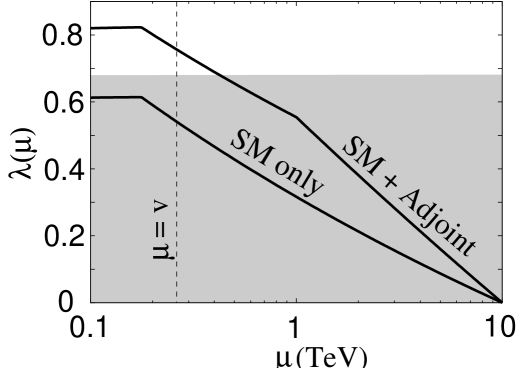
Figure 1: RG flows of the Higgs quartic coupling at 1-loop level. The UV cutoff scale $1/L$ is set to be 10 TeV. The shaded area corresponds to the LEP bound ($m_{h}\geq$ 114 GeV). The vertical line shows $\mu=\langle h\rangle=$ 246 GeV where the Higgs mass should be evaluated. The lower flow is for the case of the SM contribution only. The upper flow includes an additional fermion pairs in the adjoint representation of SU(3) with bulk mass of 1 TeV.

From this figure, we find the Higgs mass can not exceed the present experimental bound ($m_{h}\geq 114$ GeV) [19] when the compactification scale, $1/L=1/(2\pi R)^{-1}$, is smaller than 10 TeV. We can resolve the problem by increasing the compactification scale. However, it requires a finer tuning of the quadratic coupling of the Higgs field in the original GHU model, and it is not preferable (little hierarchy problem).

Therefore, we need other mechanisms to lift up the Higgs mass. A simple way is to introduce additional bulk fermions to enhance the loop correction. For instance, if we introduce $N_{a}$ adjoint fermions in the SU(3) model, the RG equation for $\lambda$ is modified as

$$\frac{d\lambda}{d\ln\mu}=\left.\frac{d\lambda}{d\ln\mu}\right|_{\rm SM}-\frac{3N_{A^{+}}}{\pi^{2}}\left\{g_{4}^{4}+2\left(\frac{g_{4}}{2}\right)^{4}\right\}~{},$$ (22)

where $g_{4}$ is the effective bulk gauge coupling, which is assumed to be the same as the SU(2) gauge coupling here. The RG flow including a couple of adjoint fermions with a 1 TeV bulk mass is also shown in Fig.1. Here, we neglect the modification of the RG equations of the gauge couplings, because the effect is at higher order level and small in the flow of the quartic coupling. This flow shows that the Higgs mass becomes large enough to be able to satisfy the LEP bound.

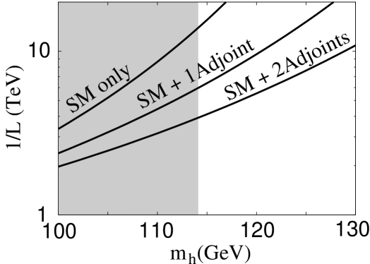
Figure 2: Relation between the Higgs mass $m_{h}$ and the compactification scale $1/L$. Again the shaded area corresponds to the LEP bound ($m_{h}\geq$ 114 GeV. The upper, middle and lower lines are for $N_{A^{+}}=0,1,2$, respectively.

In this way, we can evaluate the Higgs mass for a given compactification scale, assuming the number and representation of the bulk fermions. Conversely, we can evaluate the compactification scale from a given Higgs mass. Results are shown in Fig.2. This kind of analysis will be useful when the Higgs mass is measured. In this figure, it is also shown that the Higgs mass really becomes large as the increase of $N_{A^{+}}$, this fact is also suggested in the viewpoint of the five dimensional effective potential approach [7, 14].

V    Summary and Discussion

We have examined a general feature of low energy effective theories in the GHU scenario. In particular, we focus on the Higgs potential induced from the radiative correction through the compactification. We have shown that the low energy phenomena of GHU models can be described by the effective theory including only the zero-modes of ingredient with the specific renormalization condition, “Gauge-Higgs condition”. It is surprising that the essential informations of the GHU scenario are collected into the Gauge-Higgs condition. It means that KK modes merely acts as regulators in the GHU scenario as far as we examine the low energy physics.

In this letter, we have used the simple example, five dimensional SU(3) model, for discussing the low energy effective theory. Even if we extend the discussion to more realistic models producing the correct Weinberg angle and the large top Yukawa coupling and/or apply to more complicated setup such as a six dimensional model or a GHU model in warped extra dimension [20, 21, 22], our method would be applicable as far as the Higgs field corresponds to the degree of freedom of the Wilson line. In those cases, the Gauge-Higgs condition may be modified from Eq.(16). In fact, in the case where the shape of the extra dimension is not trivial, it is a non trivial question at which scale we should impose the condition. It is, however, still expected that the running quartic coupling should vanish at a certain scale where the four dimensional description becomes inadequate. This is because above the scale, the Higgs field behaves as the Wilson line which has vanishing potential.

This consideration may lead to the expectation that the 2-loop corrections also satisfy a similar condition that includes 1-loop threshold corrections. This is an interesting question theoretically, but this issue is beyond the scope of this letter and remains as a future problem. However, the higher loop corrections are expected to be small unless we take the setup of strongly coupled theory nor a large number of baulk matter fields.

Once we clarify the general feature of effective theories, we can use them to investigate the low energy phenomenologies of GHU models. As an example, we have made an RG improved analysis of the Higgs mass. We have shown that some mechanism for lifting up the Higgs mass is required in the realistic GHU models as far as the compactification scale is less than 10 TeV. One simple way for the lift up is to introduce bulk fermions. In this case, we may observe some massive fermions (and no scalars !!) at future collider experiments, even if no indications of the existence of extra-dimensions can not be observed. Furthermore, we can observe the flow of the running quartic coupling toward zero because of the Gauge-Higgs condition.

Acknowledgments

T.Y. would like to thank M. Tanabashi for useful discussions which become one of the motivations of this work. N.H. is supported in part by Scientific Grants from the Ministry of Education and Science, Grant No. 16028214, No. 16540258 and No. 17740150. The work of S.M. was supported in paart by a Grant-in-Aid of the Ministry of Education, Culture, Sports, Science, and Technology, Government of Japan, No. 16081211. The works of N.O. are supported in part by the Grant-in-Aid for Scientific Research (No. 15740164) from the Ministry of Education, Culture, Sports, Science, and Technology of Japan. T.Y. would like to thank the Japan Society for the Promotion of Science for financial support.

Appendix

Expansion of effective potential with bulk mass

We show the expansion formula for the contribution to the effective potential caused by periodic modes with bulk mass (S0.Ex11). For simplicity, we define dimensionless quantities as follow : $x=2\pi Q_{i}\phi$ and $z=m/L$, where $m$ is the bulk mass. For $x,z\ll 1$, the infinite sum in the contribution is expanded as

$$\sum_{w=1}^{\infty}\frac{1}{w^{5}}\left(1+wz+\frac{w^{2}z^{2}}{3}\right)e^{-wz}\cos(wx)$$ (23)

$$= \zeta_{R}(5)-\frac{\zeta_{R}(3)}{6}z^{2}+\frac{1}{32}z^{4}+\frac{1}{90}z^{5}-\frac{1}{1728}z^{6}+{\cal O}(z^{8})$$

$$+\frac{x^{2}}{2}\left(-\zeta_{R}(3)+\frac{7}{24}z^{2}+\frac{1}{288}z^{4}+{\cal O}(z^{6})\right)$$

$$+\frac{x^{4}}{4!}\frac{1}{2}\left(\frac{25}{6}+\frac{1}{36}z^{2}+{\cal O}(z^{4})\right)$$

$$-\frac{1}{4!}\frac{1}{2}(z^{2}+x^{2})^{2}\ln(z^{2}+x^{2})+{\cal O}(x^{6})~{}.$$

We can further expand the logarithm in the last line. However, the argument $z^{2}+x^{2}$ has the physical meaning, that is the mass of the zero-mode normalized by $1/L$. Thus, we keep the logarithm in the above form. Then, the infinite sum is approximated by

$$\sum_{w=1}^{\infty}\frac{1}{w^{5}}\left(1+wz+\frac{w^{2}z^{2}}{3}\right)e^{-wz}\cos(wx)$$ (24)

$$\sim \zeta_{R}(5)-\frac{x^{2}}{2}\zeta_{R}(3)-\frac{x^{4}}{4!}\frac{1}{2}\left\{\ln(z^{2}+x^{2})-\frac{25}{6}\right\}~{}.$$

Comparing with Eqs.(10) and (9), we find that the effect of the bulk mass modifies the argument of logarithm.

References

- [1] I. Antoniadis, Phys. Lett. B246 (1990), 377.
-
[2]
N. S. Manton,
Nucl. Phys. B 158, (1979), 141;
D. B. Fairlie, J. Phys. G 5, (1979), L55; Phys. Lett. B 82, (1979), 97. - [3] Y. Hosotani, Phys. Lett. B126 (1983), 309; Ann. of Phys. 190 (1989), 233; Phys. Lett. B129 (1984), 193; Phys. Rev. D29 (1984), 731.
-
[4]
N. V. Krasnikov,
Phys. Lett. B 273, (1991), 246;
H. Hatanaka, T. Inami and C. S. Lim, Mod. Phys. Lett. A 13, (1998), 2601;
G. R. Dvali, S. Randjbar-Daemi and R. Tabbash, Phys. Rev. D 65, (2002), 064021;
N. Arkani-Hamed, A. G. Cohen and H. Georgi, Phys. Lett. B 513, (2001), 232;
I. Antoniadis, K. Benakli and M. Quiros, New J. Phys. 3, (2001), 20. -
[5]
C. Csaki, C. Grojean and H. Murayama,
Phys. Rev. D 67 (2003), 085012;
G. Burdman and Y. Nomura, Nucl. Phys. B 656 (2003), 3;
N. Haba and Y. Shimizu, Phys. Rev. D 67 (2003), 095001;
I. Gogoladze, Y. Mimura and S. Nandi, Phys. Lett. B 560 (2003), 204; Phys. Lett. B 562 (2003), 307;
K. Choi, N. Haba, K. S. Jeong, K. i. Okumura, Y. Shimizu and M. Yamaguchi, JHEP 0402 (2004), 037. -
[6]
C. A. Scrucca, M. Serone and L. Silvestrini,
Nucl. Phys. B 669 (2003), 128;
G. Martinelli, M. Salvatori, C.A. Scrucca and L. Silvestrini, JHEP 0510 (2005) 037. -
[7]
N. Haba, Y. Hosotani, Y. Kawamura and T. Yamashita,
Phys. Rev. D 70 (2004), 015010;
N. Haba and T. Yamashita, JHEP 0404 (2004) 016. - [8] Y. Hosotani, S. Noda and K. Takenaga, Phys. Rev. D 69 (2004), 125014; Phys. Lett. B 607 (2005), 276.
-
[9]
M. Kubo, C. S. Lim and H. Yamashita,
Mod. Phys. Lett. A 17 (2002), 2249;
A. Delgado, A. Pomarol and M. Quiros, Phys. Rev. D 60 (1999), 095008. - [10] K. Takenaga, Phys. Lett. B 570 (2003), 244.
- [11] W. A. Bardeen, C. T. Hill and M. Lindner Phys. Rev. D 41 (1990), 1647.
- [12] Y. Kawamura, Prog. Theor. Phys. 103 (2000), 613; ibid 105 (2001), 691; ibid 105 (2001), 999.
- [13] N. Haba and T. Yamashita, JHEP 0402 (2004), 059.
- [14] N. Haba, K. Takenaga and T. Yamashita, Phys. Lett. B 615 (2005) 247.
- [15] S. Coleman and E. Weinberg, Phys. Rev. D 7 (1973), 1888.
- [16] G. Panico, M. Serone and A. Wulzer, [arXiv:hep-ph/0510373].
- [17] G. Cacciapaglia, C. Csaki and S.C. Park [arXiv:hep-ph/0510366].
- [18] H. Arason, D.J. Castano, B. Keszthelyi, S. Mikaelian, E.J. Piard, P. Ramond and B.D. Wright, Phys. Rev. D46 (1992),3945.
- [19] The ALEPH, DELPHI, L3 and OPAL Collaborations, Phys. Lett. B565, (2003), 61.
- [20] L. Randall and R. Sundrum, Phys. Rev. Lett. 83 (1999), 3370.
-
[21]
K. Oda and A. Weiler,
Phys. Lett. B 606 (2005) 408;
Y. Hosotani, M. Mabe Phys. Lett. B 615 (2005) 257. -
[22]
R. Contino, Y. Nomura and A. Pomarol,
Nucl. Phys. B 671 (2003), 148;
K. Agashe, R. Contino and A. Pomarol, Nucl. Phys. B 719 (2005), 165. - [23] C.A. Scrucca, M. Serone, L. Silvestrini and A. Wulzer, JHEP 0402 (2004) 049.