NONTRIVIAL SPACETIME TOPOLOGY,
CPT VIOLATION, AND PHOTONS

Abstract

A physical mechanism for $\mathsf{CPT}$ violation is reviewed, which relies on chiral fermions, gauge interactions, and nontrivial spacetime topology. The nontrivial topology can occur at the very largest scale (, at the “edge” of the universe) or at the very smallest scale (, from a hypothetical spacetime foam). The anomalous effective gauge field action includes, most likely, a $\mathsf{CPT}$–odd Chern–Simons-like term. Two phenomenological photon models with Abelian Chern–Simons-like terms are discussed.

11.15.-q, 04.20.Gz, 11.30.Cp, 98.70.Sa

1 Introduction

The $\mathsf{CPT}$ “theorem” [1, 2, 3, 4, 5] states that any local relativistic quantum field theory is invariant under the combined operation of charge conjugation ($\mathsf{C}$), parity reflection ($\mathsf{P}$), and time reversal ($\mathsf{T}$), in whichever order. Considered by itself, the theorem is based on the following main assumptions (cf. Ref. [4]):

• Minkowski spacetime, with manifold $\mathbb{R}^{4}$ and flat metric $\eta_{\mu\nu}$;

• invariance under transformations of the proper orthochronous Lorentz group ${\mathcal{L}}_{+}^{\uparrow}$ and spacetime translations;

• normal spin–statistics connection;

• locality and Hermiticity of the Hamiltonian.

A detailed discussion of the theorem can be found in, , Refs. [6, 7, 8] and some of its consequences have been reviewed in, , Refs. [9, 10, 11].

Here, we go further and ask the following question: can $\mathsf{CPT}$ invariance be violated at all in a physical theory and, if so, is it in the real world? It is obvious that something “out of the ordinary” is required for this to be the case. Two possibilities, in particular, have been discussed in the literature.

First, there is quantum-gravity theory, which may or may not lead to $\mathsf{CPT}$ violation; cf. Refs. [12, 13]. The point is, of course, that Lorentz invariance does not hold in general. Still, a $\mathsf{CPT}$ theorem can be “proven,” in the Euclidean formulation, for asymptotically-flat spacetimes [14]. In the canonical formulation, on the other hand, certain semiclassical (weave) states could affect the Lorentz invariance of Maxwell theory at the Planck scale and break $\mathsf{CPT}$ invariance [15, 16]. But, at the moment, this is not a firm prediction, especially as the complete theory is not formulated [17, 18].

Second, there is superstring theory, which may or may not give $\mathsf{CPT}$ violation; cf. Refs. [19, 20, 21]. The point, now, is the (mild) nonlocality of the theory. There exists, however, no convincing calculation showing the necessary violation of $\mathsf{CPT}$. And, here also, the complete theory is not formulated [22, 23, 24].

In this contribution, we discuss a third possibility: certain spacetime topologies and classes of chiral gauge theories have Lorentz and $\mathsf{CPT}$ invariance necessarily broken by quantum effects. The main article on this “$\mathsf{CPT}$ anomaly” is Ref. [25], which, under certain assumptions, finds a $\mathsf{CPT}$–odd Chern–Simons-like term in the effective gauge field action. (The connection with earlier work on sphalerons, spectral flow, and anomalies is explained in Refs. [26, 27].) Further aspects of the $\mathsf{CPT}$ anomaly have been discussed in Refs. [28, 29, 30, 31]. The corresponding Maxwell–Chern–Simons model (standard electrodynamics with an Abelian Chern–Simons-like term added to the action) has been studied in Refs. [32, 33, 34, 35, 36, 37] and a related model with random coupling constants in Refs. [38, 39]. Here, we intend to summarize the main results and to point out some of the important open questions.

The outline of the present article is as follows. In Sec. 2, a realistic example of a theory with anomalous $\mathsf{CPT}$ violation is given, together with a heuristic argument for the origin of the effect.

In Sec. 3, the $\mathsf{CPT}$ anomaly is established for a class of exactly solvable two-dimensional theories (the details are relegated to Appendix A). In Sec. 4, the existence of a $\mathsf{CPT}$ anomaly is shown nonperturbatively for a particular formulation of four-dimensional chiral lattice gauge theory (the main steps are sketched in Appendix B). In Sec. 5, the $\mathsf{CPT}$ anomaly is obtained perturbatively for a class of four-dimensional chiral gauge theories, which includes the example of Sec. 2. Two types of space manifolds are considered explicitly, a cylindrical manifold with nontrivial topology at the largest scales and a “punctured” manifold with nontrivial topology at the smallest scales.

In Sec. 6, the phenomenological Maxwell–Chern–Simons model (corresponding to the anomalous effects of a cylindrical manifold) is reviewed, while the important issue of microcausality is dealt with in Appendix C. The model Chern–Simons-like term modifies the propagation of photons, which may be relevant to photons traveling over cosmological distances (and, possibly, to the origin of the big bang). With suitable interactions added, further effects appear such as vacuum Cherenkov radiation and photon triple-splitting. In curved spacetime backgrounds, other novel phenomena occur such as stable orbits of light around a nonrotating central mass and gravitational-redshift splitting between the two polarization modes.

In Sec. 7, the phenomenology of a random-coupling photonic model (corresponding to the anomalous effects of a punctured manifold) is discussed. The resulting dispersion law has been calculated in the long-wavelength limit and can be confronted with high-energy-astrophysics data to constrain (or determine) the parameters of the photon model considered.

In Sec. 8, some concluding remarks are presented.

For the benefit of the reader, we note that this review article essentially consists of two tracks, apart from Secs. 2 and 8 with general comments. The first track focuses on the basic physics of the $\mathsf{CPT}$ anomaly and consists of Secs. 3, 4, and 5. The second track discusses nonstandard photon physics from two simple phenomenological models (the Maxwell–Chern–Simons model proper and a related photon model with random coupling constants) and consists of Secs. 6 and 7. Both tracks are more or less independent, but the second one is, of course, motivated by the first.

2 Example and heuristics

The anomalous $\mathsf{CPT}$ violation mentioned in the Introduction is perhaps best illustrated by a concrete example. Consider the following four-dimensional spacetime manifold $\mathsf{M}^{\prime}$ with metric $g_{\mu\nu}(x)$ and vierbeins $e_{\mu}^{a}(x)$:

$$\big{(}\,\mathsf{M}^{\prime}\,;\,g_{\mu\nu}(x)\,;\,e_{\mu}^{a}(x)\,\big{)}=\big{(}\,{\mathbb{R}}^{3}\times S^{1}_{\text{\,PSS}}\,;\,\eta_{\mu\nu}\,;\,\delta_{\mu}^{a}\,\big{)}\;,$$ (1)

for Minkowski tensor $(\eta_{\mu\nu})=\mathrm{diag}(1,-1,-1,-1)$, Kronecker symbol $\delta_{\mu}^{a}$, and coordinates

$$x^{0}\equiv c\,t,\,x^{1},\,x^{2}\in{\mathbb{R}}\quad\text{and}\quad x^{3}\in[0,L]\;.$$ (2)

Now take, over this cylindrical manifold $\mathsf{M}^{\prime}$, the chiral gauge field theory with group $G$ and left-handed fermion representation $R_{\text{\,left}}$ given by:

$$\big{(}\,G\,;R_{\text{\,left}}\,\big{)}=\big{(}\,SO(10)\,;\mathbf{16}+\mathbf{16}+\mathbf{16}\,\big{)}\;,$$ (3)

which incorporates the Standard Model with three families of quarks and leptons [40]. Moreover, let the fermions have periodic boundary conditions in $x^{3}$, , a periodic spin structure over $S^{1}$, as indicated by the subscript PSS in (1).

Then, for the theory as defined, quantum effects necessarily give $\mathsf{CPT}$ violation [25], with a typical mass scale

$$m_{\text{anom}}\equiv\frac{\alpha_{G}\,\hbar}{L\,c}\approx 2\times 10^{-35}\>{\rm eV}/c^{2}\,\left(\,\frac{\alpha_{G}}{1/100}\,\right)\,\left(\,\frac{10^{10}\,{\rm lyr}}{L}\,\right),$$ (4)

where $\alpha_{G}\equiv g^{2}/(4\pi)$ is defined in terms of the dimensionless $SO(10)$ gauge coupling constant $g$ and $L$ is the size of the compact dimension (here, taken as the size of the visible universe; see below). As mentioned above, this phenomenon has been called a “$\mathsf{CPT}$ anomaly,” the reason being that the $\mathsf{CPT}$ invariance of the classical theory is broken by quantum effects ($m_{\text{anom}}\propto\hbar\,$).

A heuristic argument for the existence of a $\mathsf{CPT}$ anomaly in theory (1)–(3) with appropriate gauge field configurations runs as follows [25, 26]:

• the periodic spin structure of the compact space dimension, with coordinate $x^{3}\in[0,L]$, allows for momentum component $p_{3}=0$ in a separable Dirac operator;

• a single four-dimensional chiral fermion with $p_{3}=0$ corresponds to a single massless Dirac fermion in three dimensions;

• a single massless Dirac fermion in three dimensions is known to have a “parity anomaly,” provided gauge invariance is maintained [41, 42, 43];

• this three-dimensional “parity” violation corresponds to $\mathsf{T}$ violation in the original four-dimensional theory, which, in turn, leads to $\mathsf{CPT}$ violation.

Further discussion of this particular case will be postponed till Sec. 5. Here, we continue with some general remarks.

The heuristics of the previous paragraph suggests that the $\mathsf{CPT}$ anomaly also occurs for the $SO(10)$ theory (3) over $\mathbb{R}\times S^{2}\times S^{1}_{\text{\,PSS}}$ or $\mathbb{R}\times S^{1}\times S^{1}\times S^{1}_{\text{\,PSS}}$, but not over $\mathbb{R}\times S^{3}$, where the Dirac operator is nonseparable and the space manifold $S^{3}$ simply connected. However, even over $\mathbb{R}^{3}\times S^{1}_{\text{\,PSS}}\,$, the $\mathsf{CPT}$ anomaly does not occur for standard quantum electrodynamics [44], the vector-like gauge theory of photons and electrons with $G=U(1)$ and $R_{\text{\,left}}=(1)+(-1)$. Hence, both nontrivial topology and parity violation are needed for the $\mathsf{CPT}$ anomaly.

Regarding the role of topology, the $\mathsf{CPT}$ anomaly resembles the Casimir effect, with the local properties of the vacuum depending on the boundary conditions [45, 46]. Note that the actual topology of our universe is unknown [47], but theoretically there may be some constraints (cf. Ref. [48]). Interestingly, the modification of the local physics due to the $\mathsf{CPT}$ anomaly would allow, in principle, for an indirect observation of the global spacetime structure (see Sec. 6).

Clearly, it is important to be sure of this surprising effect and to understand the mechanism better. In the next section, we, therefore, turn to a relatively simple theory, Abelian chiral gauge theory in two spacetime dimensions. From now on, we put $\hbar$ $=$ $c$ $=$ $1$, except when stated otherwise.

3 Exact result in two dimensions

Consider chiral $U(1)$ gauge theory over the flat torus $T^{2}$ $\equiv$ $S^{1}\times S^{1}$, with trivial zweibeins $e_{\mu}^{a}(x)=\delta_{\mu}^{a}$ and Euclidean metric $g_{\mu\nu}(x)\equiv e_{\mu}^{a}(x)\,e_{\nu}^{b}(x)\,\delta_{ab}=\delta_{\mu\nu}$, for diagonal matrix $(\delta_{\mu\nu})\equiv\mathrm{diag}(1,1)$. In order to be specific, take the gauge-invariant theory with five left-handed fermions of charges $(q_{f})=(1,1,1,1,-2)$ or $R_{\text{\,left}}=4\times(1)+1\times(-2)$. Furthermore, impose doubly-periodic boundary conditions on the fermions. The corresponding spin structure will be denoted PP and the specific theory $1111\overline{2}$.

The effective action $\Gamma\,[a]$ for the $U(1)$ gauge field $a_{\mu}(x)$ is defined by the functional integral

$$\exp\big{(}-\Gamma^{1111\overline{2}}_{\text{PP}}\,[a]\big{)} = \int\prod_{f=1}^{5}\left({\mathcal{D}}\bar{\psi}_{Rf}{\mathcal{D}}\psi_{Lf}\right)_{\text{PP}}\,$$ (5)

$$\times\,\exp\Big{(}-\sum_{f=1}^{5}\,\mathcal{S}_{\text{\,Weyl}}^{\,T^{2}}\left[\bar{\psi}_{Rf},\psi_{Lf},q_{f}\,a\right]\Big{)}$$

and is known exactly [49]. In fact, the effective action is given in terms of Riemann theta functions (see Appendix A).

It can now be checked explicitly that the $\mathsf{CPT}$ transformation,

$$a_{\mu}(x)\,\rightarrow\,a_{\mu}^{\mathsf{CPT}}(x)\equiv\,-a_{\mu}(-x)\,,$$ (6)

does not leave the effective action invariant [28]:

$$\Gamma^{1111\overline{2}}_{\text{PP}}\,\big{[}\,a\,\big{]}\,\rightarrow\,\Gamma^{1111\overline{2}}_{\text{PP}}\,\big{[}\,a^{\mathsf{CPT}}\,\big{]}=\,\Gamma^{1111\overline{2}}_{\text{PP}}\,\big{[}\,a\,\big{]}+\,\pi\mathrm{i}\,\pmod{2\pi\mathrm{i}\,}\;.$$ (7)

This result, which can also be understood heuristically (see Appendix A), shows unambiguously the existence of a $\mathsf{CPT}$ anomaly in this particular two-dimensional chiral $U(1)$ gauge theory. The crucial ingredients are the doubly-periodic (PP) boundary conditions and the odd number (here, five) of Weyl fermions.

4 Nonperturbative result in four dimensions

For two spacetime dimensions, we have obtained in the previous section an exact result for the effective action and established the precise form of the $\mathsf{CPT}$ anomaly, at least for appropriate boundary conditions. In four dimensions, it is, of course, not possible to calculate the effective action exactly. Still, we can establish the existence of the $\mathsf{CPT}$ anomaly by a careful consideration of the fermion measure. This will be done nonperturbatively by use of a particular lattice regularization of an Abelian chiral gauge theory.

Consider, then, the chiral $U(1)$ gauge theory consisting of a single gauge boson and sixteen left-handed fermions with $U(1)$ charges $q_{f}$, for $f=1,\ldots,16$. Specifically, the gauge group and left-handed fermion representation (, the set of left-handed charges $q_{f}$) are given by:

$$G = U(1),$$ (8a)

$$R_{\text{\,left}} = 6\times(1/3)+3\times(-4/3)+3\times(2/3)+2\times(-1)+1\times(2)$$ (8b)

$$+1\times(0)\;.$$

This particular chiral $U(1)$ gauge theory can be embedded in the $SU(2)\times U(1)$ theory relevant to the Standard Model with $U(1)$ hypercharge $Y\equiv 2\,Q-2\,T_{3}$; see, , Ref. [40]. The further embedding in the “safe” $SO(10)$ group [50] explains that the perturbative gauge anomalies cancel out for the chiral $U(1)$ gauge theory considered: $\sum_{f}(q_{f})^{3}=0$ according to Eq. (8b).

Also take a finite volume in Euclidean spacetime,

$$V=L^{\prime}\times L^{\prime}\times L^{\prime}\times L\;,$$ (9)

and introduce a regular hypercubic lattice,

$$L^{\prime}=N^{\prime}\,a\;,\quad L=N\,a\;,\qquad N^{\prime},N\in\mathbb{N}\;,$$ (10)

with lattice spacing $a$ [not to be confused with the Abelian gauge field $a_{\mu}(x)$ in the continuum]. The lattice sites have coordinates

$$(x_{1},x_{2},x_{3},x_{4})\equiv(\mathbf{x},x_{4})=(\mathbf{n}\,a,n_{4}\,a)\;,$$ (11)

for integers $n_{1},n_{2},n_{3}\in[0,N^{\prime}\,]$ and $n_{4}\in[0,N\,]$.

The spinor fields $\psi_{f}$, with flavor index $f=1,\ldots,16$, reside at the lattice sites and the vector field $U_{\mu}(x)\in U(1)$ is associated with the directed link between site $x$ and its nearest neighbor in the $\mu$–direction (that is, between sites $x$ and $x+\widehat{\mu}\,$). The boundary conditions are taken to be periodic in $x_{4}$:

$$\psi_{f}(\mathbf{x},L)=\psi_{f}(\mathbf{x},0)\;,\quad U_{\mu}(\mathbf{x},L)=U_{\mu}(\mathbf{x},0)\;,$$ (12)

mixed in $x_{1}$:

$$\psi_{f}(L^{\prime},x_{2},x_{3},x_{4}) = -\,\psi_{f}(0,x_{2},x_{3},x_{4})\>,$$

$$U_{\mu}(L^{\prime},x_{2},x_{3},x_{4}) = +\,U_{\mu}(0,x_{2},x_{3},x_{4})\>,$$ (13)

and similarly mixed in $x_{2}$ and $x_{3}$.

The specific chiral lattice gauge theory used has three main ingredients:

• Ginsparg–Wilson fermions [51];

• Neuberger’s explicit lattice Dirac operator [52];

• Lüscher’s chiral constraints [53].

Technical details for the present setup can be found in Ref. [30].

The theory is now well-defined and the Euclidean effective gauge field action $\Gamma[U]$ can, in principle, be calculated by integrating out the fermions ($U$ denotes the set of link variables). The goal is to establish the following inequality for at least one set of link variables:

$$\Gamma\big{[}\,U\,\big{]}\neq\Gamma\big{[}\,U^{\mathsf{CPT}}\,\big{]}\,,$$ (14)

with $U^{\mathsf{CPT}}$ the set of $\mathsf{CPT}$–transformed link variables.

The result (14) has been obtained in Ref. [30] for an arbitrary odd number $N$ of links in the periodic direction and for arbitrary values of the lattice spacing $a$. As the continuum limit $a\to 0$ is not needed, the result is nonperturbative. See Appendix B for a sketch of the proof.

Most importantly, the origin of the $\mathsf{CPT}$ anomaly has been identified [30] as an ambiguity in the choice of basis vectors needed to define the fermion integration measure, just as for Fujikawa’s derivation [54, 55] of the Abelian chiral anomaly (Adler–Bell–Jackiw triangle anomaly).

5 Perturbative results in four dimensions

In this section, we return to the spacetime continuum and consider the four-dimensional chiral gauge theory of Sec. 2, with

$$G=SO(10)\,,\quad R_{\text{\,left}}=N_{\mathrm{fam}}\times(\mathbf{16})\,.$$ (15)

Two four-dimensional manifolds, called $\mathsf{M}^{\prime}$ and $\mathsf{M}^{\prime\prime}$, will be discussed explicitly. From now on, the metric will have Lorentzian signature, with spacetime indices running over $0$, $1$, $2$, $3$.

5.1 Cylindrical manifold

In this subsection, we take as a prototype of nontrivial large-scale topology the cylindrical manifold discussed earlier. Specifically, consider the chiral gauge theory (15) over

$$\mathsf{M}^{\prime}=\mathbb{R}^{3}\times S^{1}_{\text{\,PSS}}\,,\quad e^{a}_{\mu}(x)=\delta^{a}_{\mu}\,,\quad(\eta_{ab})\equiv\mathrm{diag}(1,-1,-1,-1)\,,$$ (16)

where PSS stands for periodic spin structure with respect to the circle coordinate (denoted $x^{3}$ below) and the metric is the standard Minkowski metric, $g_{\mu\nu}(x)\equiv e_{\mu}^{a}(x)\,e_{\nu}^{b}(x)\,\eta_{ab}=\eta_{\mu\nu}$.

As mentioned before, the four-dimensional effective action $\Gamma[A]$, for $A$ $\in$ $\mathsf{so}(10)$, is not known exactly. But the crucial term has been identified perturbatively for an appropriate class of gauge fields (indicated by a prime), which has $A^{\prime}_{3}=0$ and $x^{3}$–independent fields in the remaining three directions. The effective action then contains the following term [25]:

$$\Gamma^{\,\mathsf{M}^{\prime}}[A^{\prime}\,]\supseteq-\int_{{\mathbb{R}}^{3}}\mathrm{d}x^{0}\mathrm{d}x^{1}\mathrm{d}x^{2}\,\int_{0}^{L}\mathrm{d}x^{3}\;\frac{n\,\pi}{L}\>\omega_{\text{\,CS}}\big{[}A^{\prime}_{0}(x),A^{\prime}_{1}(x),A^{\prime}_{2}(x)\,\big{]}\,,$$ (17)

with an integer $n$ and the standard Chern–Simons density [55]

$$\omega_{\text{\,CS}}[A_{0},A_{1},A_{2}\,]\equiv\frac{1}{16\,\pi^{2}}\;\,\epsilon^{3\kappa\lambda\mu}\;\mathrm{tr}\,\big{(}F_{\kappa\lambda}\,A_{\mu}-(2/3)\,A_{\kappa}A_{\lambda}A_{\mu}\big{)},$$ (18)

in terms of the Yang–Mills field strength [56]

$$F_{\kappa\lambda}\equiv\partial_{\kappa}A_{\lambda}-\partial_{\lambda}A_{\kappa}+A_{\kappa}A_{\lambda}-A_{\lambda}A_{\kappa}\;,$$ (19)

where the fields and their derivatives are evaluated at the same spacetime point. Here, the gauge field takes values in the Lie algebra, $A_{\mu}(x)$ $\equiv$ $A_{\mu}^{a}(x)\,T^{a}$ for $T^{a}\in\mathsf{so}(10)$ with normalization $\mathrm{tr}\,(T^{a}T^{b})$ $=$ $(-1/2)\,\delta^{ab}$, and $\epsilon^{\kappa\lambda\mu\nu}$ is the completely antisymmetric Levi-Civita symbol with $\epsilon^{1230}=1$. The indices $\kappa,\lambda,\mu$ in (18) effectively run over $0,1,2$, but the gauge fields may depend on all coordinates: $x^{0}$, $x^{1}$, $x^{2}$, and $x^{3}$. The term (17) for general gauge fields is called “Chern–Simons-like,” because a genuine topological Chern–Simons term exists only in an odd number of dimensions [55].

For gauge fields vanishing at infinity, replacing $\epsilon^{3\kappa\lambda\mu}$ in the integrand of (17) by $\partial_{\nu}x^{3}\,\epsilon^{\nu\kappa\lambda\mu}$ and integrating by parts gives the following manifestly gauge-invariant effective action:

$$\Gamma^{\,\mathsf{M}^{\prime}}[A\,]=\int_{\mathsf{M}^{\prime}}\mathrm{d}^{4}x\;\frac{n}{32\pi}\,\frac{x^{3}}{L}\;\mathrm{tr}\,\bigl{(}\epsilon^{\kappa\lambda\mu\nu}\,F_{\kappa\lambda}(x)\,F_{\mu\nu}(x)\bigr{)}+\cdots\;,$$ (20)

where the prime on $A$ has been dropped and other terms, possibly nonlocal ones, are contained in the ellipsis.

At this point, we can make three basic observations. First, the local term (20), with an explicit factor $x^{3}$ in the integrand, is clearly Lorentz noninvariant and $\mathsf{CPT}$ odd, in contrast to the Yang–Mills action [56],

$$\mathcal{S}_{\text{\,YM}}^{\,\mathsf{M}^{\prime}}=\int_{\mathsf{M}^{\prime}}\mathrm{d}^{4}x\;\frac{1}{2\,g^{2}}\;\mathrm{tr}\,\bigl{(}\eta^{\kappa\mu}\,\eta^{\lambda\nu}\,F_{\kappa\lambda}(x)\,F_{\mu\nu}(x)\bigr{)}.$$ (21)

More precisely, the Lorentz and $\mathsf{CPT}$ transformations considered are active transformations on gauge fields of local support, as discussed in Sec. IV of Ref. [28] for the two-dimensional theory. In physical terms, the wave propagation from the action (21) is essentially isotropic, whereas the term (20) makes the propagation anisotropic (see Sec. 6.2).

Second, the integer $n$ in the effective action term (20) is a remnant of the ultraviolet regularization:

$$n\equiv\sum_{f=1}^{N_{\mathrm{fam}}}\;\big{(}2\,k_{0f}+1\big{)}\;,\quad k_{0f}\in{\mathbb{Z}}\;.$$ (22)

Since the sum of an odd number of odd numbers is odd, one has $n\neq 0$ for $N_{\mathrm{fam}}=3$ and the anomalous term (20) is necessarily present in the effective action of the theory introduced in Sec. 2.

For $N_{\mathrm{fam}}=3$, the regularization of Ref. [25] gives minimally

$$n=(1-1+1)\,\Lambda_{0}\,/\,|\Lambda_{0}|=\pm\,1\;,$$ (23)

with $\Lambda_{0}$ an ultraviolet Pauli–Villars cutoff for the $x^{3}$–independent modes of the fermionic fields contributing to the effective action. [See Appendix B of Ref. [30] for a derivation of the odd integers $2k_{0f}+1$ in Eq. (22) from the lattice regularization.] The effective action term (20) has, therefore, a rather weak dependence on the small-scale structure of the theory, as shown by the factor $\Lambda_{0}/|\Lambda_{0}|$ in (23). This weak dependence on the ultraviolet cutoff has first been observed in the so-called “parity” anomaly of three-dimensional gauge theories [41, 42, 43], which underlies the four-dimensional $\mathsf{CPT}$ anomaly as discussed in Sec. 2.

Third, the $SO(10)$ theory (15) for $N_{\mathrm{fam}}=3$ has three  identical irreps (irreducible representations) and the $\mathsf{CPT}$ anomaly must occur [the integer $n$ from (22) is odd and therefore nonzero]. For the $SU(3)\times SU(2)\times U(1)$ Standard Model with $N_{\mathrm{fam}}=3$, the $\mathsf{CPT}$ anomaly may or may not occur, depending on the ultraviolet regularization. The reason is that the Standard–Model irreps come in even number (for example, four left-handed isodoublets per family), so that the integer $n$ is not guaranteed to be nonzero [$n$ is even and may or may not differ from zero]; see Sec. 5 of Ref. [25] for details. Note that the particular lattice gauge theory of Sec. 4 has all fermions regularized identically, so that the anomalous terms do not cancel.

This concludes our discussion of the $\mathsf{CPT}$ anomaly over cylindrical manifolds. Section 6 considers certain phenomenological consequences, whereas the next subsection studies the anomalous effects from a different type of manifold.

5.2 Punctured manifold

In this subsection, we take as a prototype of nontrivial small-scale topology the following “punctured” three-dimensional manifold:

$$\mathsf{M}^{\prime\prime}_{3}=\mathbb{R}\times\big{(}\mathbb{R}^{2}\setminus\{0\}\big{)}=\mathbb{R}^{3}\setminus\mathbb{R}\,.$$ (24)

The considered three-space may be said to have a linear “defect,” just as a type–II superconductor can have a single vortex line (magnetic flux tube); cf. Ref. [55]. Furthermore, introduce cylindrical coordinates $(\rho,\phi,z)$ over $\mathsf{M}^{\prime\prime}_{3}$,

$$\big{(}x^{1},\,x^{2},\,x^{3}\big{)}=\big{(}\rho\cos\phi,\,\rho\sin\phi,\,z\big{)}\,,$$ (25)

with the $z$–axis at the position of the line puncture (linear defect) and coordinate domains $\rho\in(0,\infty)$, $\phi\in[0,2\pi]$, and $z\in(-\infty,\infty)$.

The corresponding four-dimensional spacetime manifold $\mathsf{M}^{\prime\prime}=\mathbb{R}\times\mathsf{M}^{\prime\prime}_{3}$ is orientable and has flat metric $(\eta_{\mu\nu})=\mathrm{diag}(1,-1,-1,-1)$, but with nontrivial vierbeins. The particular theory considered in this subsection is, in fact, given by (15) and

$$\mathsf{M}^{\prime\prime}=\mathbb{R}\times\mathsf{M}^{\prime\prime}_{\text{3,\,PSS}}\,,\quad\big{(}e^{a}_{\mu}(x)\big{)}=\left(\begin{array}[]{cccc}1&0&0&0\\ 0&\cos\phi&-\sin\phi&0\\ 0&\sin\phi&\cos\phi&0\\ 0&0&0&1\end{array}\right)\,,$$ (26)

with the vierbeins shown in matrix notation. Again, PSS stands for periodic spin structure, but now with respect to the coordinate $\phi$. One particular class of noncontractible loops in $\mathsf{M}^{\prime\prime}_{3}$ consists of circles with fixed values of $\rho$ and $z$ (these circles are noncontractible because of the line removed from $\mathbb{R}^{3}$, which happens to coincide with the $z$ axis of the coordinates used).

For our purpose, it suffices to establish the $\mathsf{CPT}$ anomaly for one particular class of gauge fields. Take the four-dimensional gauge fields over $\mathsf{M}^{\prime\prime}$ to be independent of $\phi$ and without component in the direction of $\phi$. These fields will be indicated by a double prime in the following. The anomalous contribution to the effective action is then found to be given by [31]

$$\Gamma^{\,\mathsf{M}^{\prime\prime}}[A^{\prime\prime}\,]\supseteq\int_{\mathsf{M}^{\prime\prime}}\!\mathrm{d}^{4}x\,\,\,\frac{n}{32\pi}\;\frac{\phi(x)}{2\pi}\;\;\mathrm{tr}\,\bigl{(}\epsilon^{\kappa\lambda\mu\nu}\,F^{\prime\prime}_{\kappa\lambda}(x)\,F^{\prime\prime}_{\mu\nu}(x)\bigr{)}\,,$$ (27)

where $\phi(x)$ denotes the azimuthal angle from (25), measured with respect to the linear defect of $\mathsf{M}^{\prime\prime}_{3}$. The long-range anomalous effects occur already for an infinitely thin linear defect, which is not the case for standard electromagnetic propagation effects. Furthermore, the anomalous term (27) from nontrivial small-scale topology (noncontractible loops with arbitrarily small lengths) has the same structure as (20) from nontrivial large-scale topology (noncontractible loops with lengths equal to or larger than $L$). A result similar to (27) has been obtained heuristically [31] for a space manifold $\mathbb{R}^{3}$ with two points identified, which is a simplified version of a permanent static “wormhole” [57, 58].

The general structure of the anomalous term (27) for an arbitrary flat manifold $\mathsf{M}$ with a single puncture (or wormhole) has the following form:

$$\Gamma^{\,\mathsf{M}}[A\,]=\int_{\mathbb{R}^{4}}\!\mathrm{d}^{4}x\,\,f_{\mathsf{M}}(x;A]\;\;\mathrm{tr}\,\bigl{(}\epsilon^{\kappa\lambda\mu\nu}\,F_{\kappa\lambda}(x)\,F_{\mu\nu}(x)\bigr{)}+\cdots\,,$$ (28)

where $F_{\mu\nu}$ stands for the Yang–Mills field strength (19) and the integration domain has been extended to $\mathbb{R}^{4}$, which is possible for smooth enough gauge fields $A_{\mu}(x)$. The factor $f_{\mathsf{M}}(x;A]$ is both a function of the spacetime coordinates $x^{\mu}$ and a gauge-invariant functional of the gauge field $A_{\mu}(x)$. This functional dependence of $f_{\mathsf{M}}$ involves, most likely, the gauge field holonomies. But the functional $f_{\mathsf{M}}(x;A]$ is not known in general.

This concludes our brief discussion of the $\mathsf{CPT}$ anomaly over a manifold with a single puncture. The calculation with two or more punctures (or wormholes) is, however, difficult and a simple phenomenological model will be introduced in Sec. 7.

6 Maxwell–Chern–Simons model and phenomenology

6.1 MCS action and microcausality

Starting from the four-dimensional continuum theory of Sec. 5.1, we consider the electromagnetic $U(1)$ gauge field $a_{\mu}(x)$ embedded in the $SO(10)$ gauge field $A_{\mu}(x)$. Also, we extend the cylindrical manifold $\mathsf{M}^{\prime}$ to Minkowski spacetime ${\mathbb{R}}^{4}$ with metric $(\eta_{\mu\nu})=\mathrm{diag}(1,-1,-1,-1)$. In effect, we take the double limit $L\to\infty$ and $n\to\infty$ of (17) and (21), with constant ratio $n/L$. For most of this section, we will suppress the explicit spacetime dependence of the fields.

For electromagnetic fields $a_{\mu}$ of local support and after appropriate rescaling, the following local terms can be expected to be present in the effective action:

$$\mathcal{S}_{\text{\,MCS}} = \mathcal{S}_{\text{\,M}}+\mathcal{S}_{\text{\,CS}}\;,$$ (29)

$$\mathcal{S}_{\text{\,M}} = \int_{{\mathbb{R}}^{4}}\mathrm{d}^{4}x\;\big{(}-(1/4)\,\eta^{\kappa\mu}\,\eta^{\lambda\nu}\,f_{\kappa\lambda}\,f_{\mu\nu}\big{)}\;,$$ (30)

$$\mathcal{S}_{\text{\,CS}} = \int_{{\mathbb{R}}^{4}}\mathrm{d}^{4}x\;\big{(}+(1/4)\,m\,\epsilon^{3\kappa\lambda\mu}\,f_{\kappa\lambda}\,a_{\mu}\big{)}\;,$$ (31)

with Maxwell field strength

$$f_{\mu\nu}\equiv\partial_{\mu}a_{\nu}-\partial_{\nu}a_{\mu}$$ (32)

and Chern–Simons mass parameter $m\geq 0$ [in terms of the previous parameters: $m\sim\alpha\,n/L$, with fine-structure constant $\alpha\equiv e^{2}/(4\pi)$ and $e\sim g$].

The Maxwell–Chern–Simons (MCS) model per se has been studied before, in particular, by the authors of Refs. [59, 60, 61]. The action (29) is gauge invariant, provided the electric and magnetic fields in $f_{\kappa\lambda}$ vanish fast enough at infinity. The gauge invariance of the Chern–Simons-like term (31) makes clear that the parameter $m$ is not simply the mass of the photon [62], it affects the propagation in a different way (see Sec. 6.2).

On the other hand, there is known to be a close relation [5, 6, 7, 8] between $\mathsf{CPT}$ invariance and microcausality, , commutativity of local observables with spacelike separations. The question is then whether or not causality holds in the $\mathsf{CPT}$–violating MCS model. Remarkably, microcausality (locality) can be established also in the particular MCS model considered [32]. The commutation relations are given in Appendix C.

The topics discussed in the remainder of this section include the propagation properties of MCS photons and their interactions with conventional electrons and gravitational fields. Note that, even though certain results are obtained for classical waves, we will speak freely about “photons,” assuming that the complete quantization procedure can be performed successfully [34, 63].

6.2 MCS photons in flat spacetime

The propagation of electromagnetic waves in the Maxwell–Chern–Simons (MCS) model (29) makes clear that $\mathsf{C}$ and $\mathsf{P}$ are conserved, but $\mathsf{T}$ not. An example is provided by the behavior of pulses of circularly polarized light, as will be shown in this subsection.

The dispersion law for plane electromagnetic waves in the MCS model is given by [32, 59, 60, 61]:

$$\omega_{\,\pm}^{2}\equiv k_{1}^{2}+k_{2}^{2}+\bigl{(}q_{3}\pm m/2\bigr{)}^{2}\;,\quad q_{3}\equiv\sqrt{k_{3}^{2}+m^{2}/4}\;,$$ (33)

where the suffix $\pm$ labels the two different modes (denoted $\oplus$ and $\ominus$, respectively). The phase and group velocities are readily calculated from this dispersion law,

$$\mathbf{v}_{\rm ph}^{\,\pm}\equiv\bigl{(}k_{1},k_{2},k_{3}\bigr{)}\,\frac{\omega_{\,\pm}}{|\mathbf{k}\,|^{2}}\;,\quad\mathbf{v}_{\rm g}^{\,\pm}\equiv\left(\frac{\partial}{\partial k_{1}}\,,\frac{\partial}{\partial k_{2}}\,,\frac{\partial}{\partial k_{3}}\,\right)\omega_{\,\pm}\;.$$ (34)

The magnitudes of the group velocities turn out to be given by (recall $c\equiv 1$):

$$|\mathbf{v}_{\rm g}^{\,\pm}(k_{1},k_{2},k_{3})|^{2}=\frac{k_{1}^{2}+k_{2}^{2}+\bigl{(}q_{3}\pm m/2\bigr{)}^{2}\,k_{3}^{2}/q_{3}^{2}}{k_{1}^{2}+k_{2}^{2}+\bigl{(}q_{3}\pm m/2\bigr{)}^{2}}\leq 1\;,$$ (35)

with equality for $m=0$ or for a $\ominus$–mode having $k_{3}=0$ (recall $m\geq 0$).

For our purpose, it is necessary to obtain the explicit polarizations of the electric and magnetic fields (see Refs. [34, 36] for further details). As long as the propagation of the plane wave is not exactly along the $x^{3}$ axis, the radiative electric field can be expanded as follows ($\Re$ denotes taking the real part):

$$\mathbf{E}_{\,\pm}(\mathbf{x},t) = \Re\,\Big{(}c^{\,\pm}_{1}\;\big{(}\,\widehat{\mathbf{e}}_{3}-(\,\widehat{\mathbf{e}}_{3}\cdot\widehat{\mathbf{k}}\,)\>\widehat{\mathbf{k}}\,\big{)}+c^{\,\pm}_{2}\;\big{(}\,\widehat{\mathbf{e}}_{3}\times\widehat{\mathbf{k}}\,\big{)}+c^{\,\pm}_{3}\;\widehat{\mathbf{k}}\,\Big{)}$$ (36)

$$\times\exp\left[\,\mathrm{i}\,(\mathbf{k}\cdot\mathbf{x}-\omega_{\,\pm}\,t)\,\right],$$

with unit vector $\widehat{\mathbf{e}}_{3}$ in the preferred $x^{3}$–direction, unit vector $\widehat{\mathbf{k}}$ corresponding to the wave vector $\mathbf{k}\,$, polar angle $\theta$ of the wave vector (so that $k_{3}\equiv\mathbf{k}\cdot\widehat{\mathbf{e}}_{3}=|\mathbf{k}|\,\cos\theta$), and complex coefficients $c^{\,\pm}_{1}$, $c^{\,\pm}_{2}$, and $c^{\,\pm}_{3}$ (at this point, the overall normalization is arbitrary). The vacuum MCS field equations then give the following polarization coefficients for the two modes:

$$\left(\begin{array}[]{c}c^{\,\pm}_{1}\\[2.84526pt] c^{\,\pm}_{2}\\[2.84526pt] c^{\,\pm}_{3}\end{array}\right)=\left(\begin{array}[]{c}\cos\theta\left(\sqrt{\cos^{2}\theta+\mu_{\,\pm}^{2}\sin^{4}\theta}\,\pm\,\mu_{\,\pm}\,\sin^{2}\theta\right)^{-1}\\ \pm\,\mathrm{i}\\[2.84526pt] \mp\,2\,\mu_{\,\pm}\,\sin^{2}\theta\end{array}\,\right)\;,$$ (37)

with $\mu_{\,\pm}\equiv m/(2\,\omega_{\,\pm})\geq 0$ for positive frequencies $\omega_{\,\pm}$ from Eq. (33). The corresponding magnetic field is

$$\mathbf{B}_{\,\pm}=\bigl{(}\,\mathbf{k}\,\times\mathbf{E}_{\,\pm}\,\bigr{)}/\,\omega_{\,\pm}\;.$$ (38)

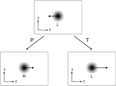
Figure 1: Sketch of the behavior of a left-handed wave packet in the Maxwell–Chern–Simons model (29) under the time reversal ($\mathsf{T}$) and parity ($\mathsf{P}$) transformations. [The charge conjugation ($\mathsf{C}$) transformation acts trivially.] The nonzero energy density of the pulse is indicated by the shaded area and the arrow shows the group velocity approximately along a “standard” direction with coordinate $x^{2}$, for the case of a “preferred” direction with coordinate $x^{3}$. The magnitude of the group velocity changes under $\mathsf{T}$, but not under $\mathsf{C}$ or $\mathsf{P}$. Hence, the physics is $\mathsf{CPT}$–noninvariant. In addition, the vacuum is seen to be optically active, with left- and right-handed light pulses traveling to the right at different speeds (the same holds for pulses traveling to the left).

As long as the $\mu_{\,\pm}\sin^{2}\theta$ terms in (37) are negligible compared to $|\cos\theta|$, the transverse electric field consists of the standard circular polarization modes (see below). For the opposite case, $|\cos\theta|$ negligible compared to $\mu_{\,\pm}\sin^{2}\theta$, the transverse polarization ($c^{\,\pm}_{1}$, $c^{\,\pm}_{2}$) becomes effectively linear.

Now consider the propagation of light pulses close to the $x^{2}$ axis. For $k_{1}=0$ and $0<m\ll|k_{3}|\ll|k_{2}|$, in particular, we can identify the $\oplus/\ominus$–modes of the dispersion law (33) with left- and right-handed circularly polarized modes ($L$ and $R\,$; cf. Ref. [64]), depending on the sign of $k_{3}\equiv|\mathbf{k}|\,\cos\theta$. From Eqs. (36) and (37), one obtains that $\oplus/\ominus$ corresponds to $R/L$ for $k_{3}>0$ and to $L/R$ for $k_{3}<0$.

With these identifications, Eq. (35) gives the following relations for the group velocities of pulses of circularly polarized light ($m\ll|k_{3}|\ll|k_{2}|$):

$$|\,\mathbf{v}^{\,L}_{\mathrm{g}}(0,k_{2},k_{3})| = |\,\mathbf{v}^{\,R}_{\mathrm{g}}(0,-k_{2},-k_{3})|\;,$$ (39a)

$$|\,\mathbf{v}^{\,L}_{\mathrm{g}}(0,k_{2},k_{3})| \neq |\,\mathbf{v}^{\,L}_{\mathrm{g}}(0,-k_{2},-k_{3})|\;,$$ (39b)

provided $m\neq 0$. Recall, at this point, that the time-reversal operator $\mathsf{T}$ reverses the direction of the wave vector and leaves the helicity unchanged, whereas the parity-reflection operator $\mathsf{P}$ flips both the wave vector and the helicity. Equality (39a) is, therefore, consistent with parity invariance, while inequality (39b) implies time-reversal noninvariance for this concrete physical situation (see Fig. 1).

The velocities (34)–(35) show that the vacuum has become optically active (see also Fig. 1). In particular, left- and right-handed monochromatic plane waves travel at different speeds [59]. (This effect has also been noticed by the authors of Ref. [65] in the context of axionic domain walls.) In the following two subsections, we discuss two “applications” of MCS optical activity or birefringence.

6.3 Cosmic microwave background

In the previous subsection, we have seen that the MCS vacuum is optically active. As mentioned in Ref. [25], this may, in principle, lead to observable effects of the $\mathsf{CPT}$ anomaly in the cosmic microwave background (CMB): the polarization pattern around hot-spots and cold-spots is modified due to the action of the Chern–Simons-like term (31) on the electromagnetic waves traveling between the last-scattering surface (redshift $z$ $\sim$ $10^{3}$) and the detector ($z$ $=$ $0$). Figure 2 gives a sketch of this cosmic birefringence effect, which can be looked for by ESA’s Planck Surveyor and next-generation satellite experiments (perhaps CMBPOL). See Ref. [66] for a pedagogical review of the expected CMB polarization and Ref. [67] for further details on the possible signatures of cosmic birefringence from a spacelike Chern–Simons vector (a timelike Chern–Simons vector was considered in Ref. [68]).

It is important to realize that the optical activity from the $\mathsf{CPT}$ anomaly, as illustrated by Fig. 2, is essentially frequency independent, in contrast to the quantum-gravity effects suggested by the authors of, for example, Refs. [15, 16]. Quantum-gravity effects on the photon propagation can generally be expected to become more and more important as the photon energy increases towards $E_{\text{\,Planck}}\equiv(\hbar\,c^{5}/G)^{1/2}\approx 1.2\times 10^{19}\,\text{GeV}$. The potential $\mathsf{CPT}$–anomaly effect at the relatively low CMB photon energies ($\hbar\,\omega\sim 10^{-4}\,\text{eV}$) is, therefore, quite remarkable. Indeed, the weak ultraviolet-cutoff dependence of the $\mathsf{CPT}$ anomaly has already been commented on a few lines below Eq. (23).

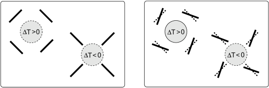
Figure 2: Sketch of the linear polarization pattern (indicated by heavy bars) around cosmic-microwave-background hot-spots ($\Delta T>0$) and cold-spots ($\Delta T<0$), generated by scalar perturbations of the metric. The left panel is in a “standard” direction with Cartesian coordinate $x^{1}$ or $x^{2}$. The right panel is in the “preferred” direction with coordinate $x^{3}$ and displays the optical activity of the Maxwell–Chern–Simons model (29) considered. In fact, for a patch of sky in a particular direction along the $x^{3}$ axis (shown in the right panel), the linear polarization pattern is rotated by a very small amount in the counterclockwise direction. For a patch of sky in the opposite direction (not shown), the rotation of the linear polarization is in the clockwise direction.

6.4 Big bang vs. big crunch

In this subsection, we turn to an entirely different application of MCS photons, namely as an ingredient of a Gedankenexperiment. The problem addressed, the arrow of time, is one of the most profound of modern physics and we refer to the clear discussion given by Penrose [69]; further references can be found in, , Ref. [70].

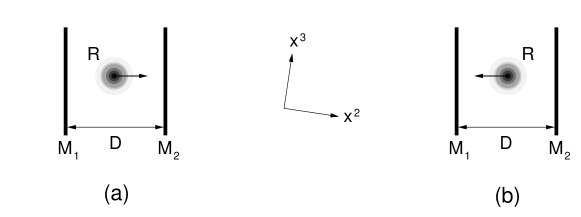
Figure 3: (a) Sketch of clock $C$, with a single pulse of circularly polarized light reflecting between two parallel mirrors, $M_{1}$ and $M_{2}$, at a fixed distance $D$. Shown is the time at which the clock is started, with a right-handed ($R$) light pulse moving towards the right (, in the direction of increasing $x^{2}$). (b) Sketch of clock $C^{\prime}$, which has all motions reversed compared to clock $C$. Clock $C^{\prime}$ starts with a right-handed light pulse moving towards the left.

Figure 4: (a) Spacetime diagram of clock $C$ in the MCS model (29), with ticks $\Delta t$ between the successive reflections of the light pulse. The slight offset in the $x^{3}$–direction, as indicated by Fig. 3, is not shown here. (b) Spacetime diagram of clock $C^{\prime}$, with ticks $\Delta t^{\prime}$.

After examining the various time-asymmetries present at the macroscopic level, Penrose asked the basic question: “what special geometric structure did the big bang possess that distinguishes it from the time-reverse of the generic singularities of collapse—and why?”

He then proposed a particular condition (the vanishing of the Weyl curvature tensor) to hold at any initial singularity. Whatever the precise condition may be, the crucial point is that this condition would not hold for final singularities. This implies that the unknown physics responsible for the “initial singularity” necessarily involves $\mathsf{T}$, $\mathsf{PT}$, $\mathsf{CT}$, and $\mathsf{CPT}$ violation; see Sec. 12.4 of Ref. [69].

But Penrose did not make a concrete proposal for the physical mechanism of this $\mathsf{T}$ and $\mathsf{CPT}$ noninvariance. In Ref. [35], the possible relevance of the $\mathsf{CPT}$ anomaly was suggested, which does not involve gravitation directly but does depend on the global structure (topology) of space.

Consider the light clock $C$ of Figs. 3a and 4a. The decisive point, now, is that the time-reversed copy $C^{\prime}$ of Figs. 3b and 4b runs differently in the effective MCS model (29), as discussed in Sec. 6.2.

More fundamentally, consider the $SO(10)$ chiral gauge theory (3) in a homogeneous Kantowski–Sachs universe [48, 71, 72] with spacetime topology ${\mathbb{R}}\times S^{2}\times S^{1}_{\text{\,PSS}}$, which re-collapses after a period of expansion and has anomalous $\mathsf{CPT}$ violation. The clock $C$ near the big bang and the time-reversed copy of clock $C$ (, clock $C^{\prime}$) near the big crunch then give a different number of ticks over an equal time interval as defined by a standard clock (or by the expansion and contraction of the universe). The setup is sketched in Fig. 5. (See also Ref. [73] for a related discussion of a $K^{0}$–beam with hypothetical $\mathsf{CPT}$ violation in a re-collapsing universe.)

Figure 5: Clocks $C$ and $C^{\prime}$ in a Kantowski–Sachs universe with expansion factor $a$ as a function of cosmic time $t$ and re-collapse time $\tau$. The background metric is invariant under time reversal ($\mathsf{T}$) but the clock $C$ made from MCS photons not.

Therefore, the physics near the initial singularity and the physics near the final singularity could be different, as demonstrated by this Gedankenexperiment with MCS photons in a Kantowski–Sachs universe [35]. Of course, the potential effect discussed gives only a “direction in time” and the main dynamics of the big-bang singularity still needs to be explained. In a way, the situation would be analogous to spontaneous magnetization in ferromagnets, where a small impurity or boundary effect determines the direction in space of the magnetization in the domain considered but the dynamics is really driven by the spin interactions.

6.5 Decay processes in modified QED

In this subsection, we consider new two- and three-particle decay processes [36] in the Maxwell–Chern–Simons model with conventional electrons added. Using the inverse Minkowski metric $(\eta^{\mu\nu})\equiv\mathrm{diag}(1,-1,-1,-1)$ to raise indices and to define $\gamma^{\mu}\gamma^{\nu}+\gamma^{\nu}\gamma^{\mu}=\eta^{\mu\nu}$, the relevant action of this particular modification of quantum electrodynamics (QED) is given by

$$\mathcal{S}_{\text{\,modified\;QED}}=\mathcal{S}_{\,\text{MCS},\;\xi^{\mu}\xi_{\mu}=-1\;,\;\xi^{0}=0}\>+\mathcal{S}_{\,\text{D}}\;\text{,}$$ (40)

with the Maxwell–Chern–Simons (MCS) terms

$$\mathcal{S}_{\,\text{MCS},\;\xi^{\mu}}=\int_{{\mathbb{R}}^{4}}\mathrm{d}^{4}x\;\big{(}\,-(1/4)\,f_{\mu\nu}\,f^{\mu\nu}+(1/4)\;\,m\,\epsilon_{\mu\nu\rho\sigma}\,\xi^{\,\mu}\,a^{\nu}\,f^{\rho\sigma}\,\big{)}\text{,}$$ (41)

and the standard Dirac term [44]

$$\mathcal{S}_{\,\text{D}}=\int_{\mathbb{R}^{4}}\mathrm{d}^{4}x\;\bar{\psi}\,\big{(}\,\mathrm{i}\,\gamma^{\mu}\partial_{\mu}-M-e\,\gamma^{\mu}a_{\mu}\big{)}\,\psi\text{,}$$ (42)

where the electron from field $\psi$ has charge $e$ and mass $M>m/2>0$. Remark that the normalized (dimensionless) Chern–Simons vector $\xi^{\mu}$ has been taken to be purely spacelike in (40) and that the corresponding spatial vector $\boldsymbol{\xi}$ was previously taken to point in the $x^{3}$–direction, as shown by (31). Note also that $\xi^{\mu}$ was written as $\widehat{\zeta}^{\mu}$ in Ref. [36]. The two polarization modes of the MCS photon are again denoted $\oplus/\ominus$, corresponding to the $+/-$ sign in the dispersion law (33).

First, we discuss the Cherenkov process $e^{-}\to\ominus\,e^{-}$, which occurs already at tree level and is allowed for any three-momentum $\mathbf{q}$ of the electron, provided $\mathbf{q}$ has a nonzero component in the $\boldsymbol{\xi}$–direction. The process $e^{-}\to\oplus\,e^{-}$ is not allowed kinematically. (See, , Refs. [74, 75] for a general discussion of vacuum Cherenkov radiation and Ref. [76] for a discussion in the context of the MCS model.)

The tree-level amplitude $A$ for $e^{-}\to\ominus\,e^{-}$ follows directly from the QED interaction (42),

$$A=\bar{u}(q-k)\,\bar{\epsilon}_{\mu}(k)\,(-e\gamma^{\mu})\,u(q)\text{,}$$ (43)

with $u$ the incoming and $\bar{u}$ the outgoing spinor and $\bar{\epsilon}_{\mu}$ the conjugate polarization vector of the MCS photon. The corresponding Feynman diagram is shown in the left panel of Fig. 6. (The Feynman rules of standard QED are given in, for example, Ref. [44].)

Figure 6: Feynman diagrams contributing to vacuum Cherenkov radiation (left panel) and photon triple-splitting (right panel) in the Maxwell–Chern–Simons model with conventional Dirac fields added.

An analytic calculation gives the following Cherenkov decay width [36]:

$$\Gamma(\mathbf{q})=\frac{1}{2\,\sqrt{|\mathbf{q}|^{2}+M^{2}}}\;\gamma(q_{\parallel})\text{,}$$ (44)

with decay parameter $\gamma$ as a function of the parallel momentum $q_{\parallel}\equiv\mathbf{q}\cdot\boldsymbol{\xi}$:

$$\gamma(q_{\parallel})=\;\frac{\alpha}{16\,\sqrt{q_{\parallel}^{2}+M^{2}}}\,\Big{[}\,8m^{2}\,|q_{\parallel}|-2m\,\big{(}4\,|q_{\parallel}|-k_{\text{max}}\big{)}\,\sqrt{m^{2}+4k_{\text{max}}^{2}}$$

$$-4\left(m^{2}+4M^{2}\right)k_{\text{max}}+m\big{(}m^{2}+8M^{2}+16\,q_{\parallel}^{2}\,\big{)}\,\text{arcsinh}\Big{(}\,\frac{2\,k_{\text{max}}}{m}\,\Big{)}\Big{]}\text{,}$$ (45)

for fine-structure constant $\alpha\equiv e^{2}/(4\pi)$ and maximum parallel photon momentum $k_{\text{max}}$ defined by

$$k_{\text{max}}(q_{\parallel})\equiv\frac{{2m\,|q_{\parallel}|\,\left(m+2\,\sqrt{q_{\parallel}^{2}+M^{2}}\,\right)}_{\vphantom{!_{a}}}}{{m^{2}+4M^{2}+4m\,\sqrt{q_{\parallel}^{2}+M^{2}}}^{\vphantom{a}}}\;\geq\,0\,\text{.}$$ (46)

For $0\leq|q_{\parallel}|<M$, the result (6.5) can be expanded in $m/M$,

$$\gamma(q_{\parallel})=(4/3)\,\alpha\;m\,|q_{\parallel}|^{3}/M^{2}+\mathrm{O}\left(\alpha\,m^{2}\,|q_{\parallel}|^{3}/|M|^{3}\,\right)\text{,}$$ (47)

while, for $|q_{\parallel}|\gg M$, an expansion in $m/|q_{\parallel}|$ and $M/|q_{\parallel}|$ gives

$$\gamma(q_{\parallel})=\alpha\,m\,|q_{\parallel}|\,\big{(}\ln(|q_{\parallel}|/m)+2\ln 2-3/4\,\big{)}+\cdots\,\text{,}$$ (48)

where the ellipsis stands for subdominant terms. Hence, the decay parameter of the electron grows approximately linearly with the momentum component in the preferred direction, but is suppressed by one power of $m$. For $|\mathbf{q}|\to\infty$ and fixed angle $\theta\neq\pi/2$ between $\mathbf{q}$ and $\boldsymbol{\xi}$, the decay rate (44) behaves as follows:

$$\Gamma(\mathbf{q})\sim(1/2)\>\alpha\,m\,|\cos\theta|\;\ln\big{(}|\mathbf{q}|/m\big{)}\text{,}$$ (49)

where the definition $q_{\parallel}\equiv\mathbf{q}\cdot\boldsymbol{\xi}\equiv|\mathbf{q}|\cos\theta$ has been used and only the leading term in $|\mathbf{q}|$ has been shown.

Next, we discuss photon triple-splitting in the purely spacelike MCS model (41), which was first considered in Ref. [34] and then generalized in Ref. [36]. There are eight decay channels, corresponding to all possible combinations of $\oplus$–modes and $\ominus$–modes. It can be shown that the following three channels are allowed for generic initial three-momentum $\mathbf{q}$: $\oplus\to\ominus\ominus\ominus$, $\oplus\to\oplus\ominus\ominus$, and $\ominus\to\ominus\ominus\ominus$, whereas the five others are kinematically forbidden. For special momentum $\mathbf{q}\perp\boldsymbol{\xi}$, only the decay channel $\oplus\to\ominus\ominus\ominus$ is available.

The implication would be that, with suitable interactions, all MCS photons are generally unstable against splitting. The exception would be for the lower-dimensional subset of $\ominus$–modes with three-momenta orthogonal to $\boldsymbol{\xi}$.

The interaction is now taken to be the Euler–Heisenberg interaction and the photonic action considered reads

$$\mathcal{S}_{\text{photon}} =\mathcal{S}_{\text{MCS},\;\xi^{\mu}\xi_{\mu}=-1\;,\;\xi^{0}=0}+\mathcal{S}_{\text{EH}}\text{,}$$ (50)

consisting of the quadratic MCS terms (41), for purely spacelike background four-vector $\xi^{\mu}$, and the quartic Euler–Heisenberg term

$$\mathcal{S}_{\text{EH}}=\frac{2\alpha^{2}}{45M^{4}}\int_{\mathbb{R}^{4}}\mathrm{d}^{4}x\,\left[\,\big{(}\,(1/2)\,f_{\mu\nu}f^{\mu\nu}\big{)}^{2}+7\,\big{(}\,(1/8)\,\epsilon_{\mu\nu\rho\sigma}f^{\mu\nu}f^{\rho\sigma}\big{)}^{2}\,\right]\text{,}$$ (51)

with fine-structure constant $\alpha\equiv e^{2}/(4\pi)$ and electron mass $M$. For modified QED with action (40), the Euler–Heisenberg term arises from the low-energy limit of the one-loop electron contribution to the effective gauge field action [44]; see also the right panel of Fig. 6.

The decay width of photon triple-splitting in model (50) is then given by [36]:

$$\Gamma(\mathbf{q})=\frac{1}{2\,\omega(\mathbf{q})}\;\gamma(q_{\parallel})\text{,}$$ (52)

with the following behavior of the decay parameter for $|q_{\parallel}|\gg m$:

$$\gamma(q_{\parallel})\sim c\;\alpha^{4}\;m^{5}\;|q_{\parallel}|^{5}/M^{8}\text{.}$$ (53)

The numerical constant $c$ in (53) depends on the decay channel ($\oplus\to\ominus\ominus\ominus$, $\oplus\to\oplus\ominus\ominus$, or $\ominus\to\ominus\ominus\ominus$) and ranges between $1.23\times 10^{-10}$ and $2.33\times 10^{-10}$.

Finally, let us comment on the possible high-energy behavior of photon triple-splitting in modified QED with action (40), as our calculation in model (50) was only valid for momenta less than $M^{2}/m$, with an extra factor $M/m$ compared to the naive expectation $M$ [36]. Recall that, for standard QED, the $\mathrm{O}(\alpha^{2})$ amplitude of a four-photon interaction is known in principle [44].

Consideration of the amplitude and phase space integral suggests the following behavior for the decay parameter of the process shown in the right panel of Fig. 6:

$$\gamma\;\big{|}_{\;|q_{\parallel}|\gg M^{2}/m}\stackrel{{\scriptstyle?}}{{\sim}}\;c_{\infty}\,\alpha^{4}\,m\,|q_{\parallel}|\,\text{,}$$ (54)

neglecting logarithms of $|q_{\parallel}|$. Combined with the “low-energy” result (53), this would imply that the effect of Lorentz breaking continues to grow with energy. At ultra-high energies, the decay rate (52) would then approach a direction-dependent constant (up to logarithms). A similar behavior has been seen for vacuum Cherenkov radiation in (49).

6.6 MCS photons in curved spacetime backgrounds

The MCS model (29) can also be coupled to gravity. One possibility for the coupling is given by the following generalized action [37, 77]:

$$\mathcal{S} = \mathcal{S}^{\text{grav.}}_{\text{EH}}+\mathcal{S}^{\text{gen.}}_{\text{MCS}}+\cdots\,,$$ (55)

$$\mathcal{S}^{\text{grav.}}_{\text{EH}} = \int\mathrm{d}^{4}x\;e\medspace R/(16\pi G)\,,$$ (56)

$$\mathcal{S}^{\text{gen.}}_{\text{MCS}} = \int\mathrm{d}^{4}x\;\left(-\frac{1}{4}\,e\,g^{\kappa\mu}g^{\lambda\nu}\,f_{\kappa\lambda}\,f_{\mu\nu}+\frac{1}{4}\,m\;\xi_{a}e_{\kappa}^{\;a}\,\epsilon^{\kappa\lambda\mu\nu}f_{\lambda\mu}\,a_{\nu}\right)\,,$$ (57)

for the case of a Cartan connection $\Gamma^{\lambda}_{\;\mu\nu}=\Gamma^{\lambda}_{\;\nu\mu}$ (, a torsion-free theory [78]), so that the standard definition (32) of the field strength $f_{\mu\nu}$ still holds. Note that $\xi_{a}$ was written as $-\zeta_{a}$ in Ref. [37]. In addition, $g_{\mu\nu}(x)$ is the metric with signature $(+\,-\,-\,-\,)$, $e_{\kappa}^{\;a}(x)$ the vierbeins with $e(x)\equiv\det e_{\kappa}^{\;a}(x)$, $R$ the Ricci curvature scalar which enters the Einstein–Hilbert action (56) with a coupling proportional to the inverse of Newton’s constant $G$, and $\epsilon^{\kappa\lambda\mu\nu}$ the Levi–Civita tensor density.

The combined action from Eqs. (56) and (57) is, however, not satisfactory [77] and further contributions are needed, hence the ellipsis in Eq. (55). For the moment, we only consider the light-propagation effects from the MCS action (57) in given spacetime backgrounds.

The condition $\partial_{b}\,\xi^{a}=0$ holds for the flat MCS model and the covariant generalization $D_{\mu}\xi_{\nu}=0$ might seem natural. But this condition imposes strong restrictions on the curvature of the spacetime [77] and it may be better to demand only closure [59],

$$D_{\mu}\xi_{\nu}-D_{\nu}\xi_{\mu}=\partial_{\mu}\xi_{\nu}-\partial_{\nu}\xi_{\mu}=0.$$ (58)

This last requirement ensures, at least, the gauge invariance of action (57). Furthermore, we assume that the norm of $\xi^{\mu}$ is constant, $\xi_{\mu}\xi^{\mu}=-1$, in order to simplify the calculations.

The geometrical-optics approximation of the MCS model (57) in a curved spacetime background has been studied in Ref. [37]. The main result there is the derivation of a modified geodesic equation, starting from the equation of motion of the gauge field,

$$e\,D_{\mu}f^{\mu\nu}=(1/2)\,m\,\xi_{\kappa}\,\epsilon^{\kappa\nu\rho\sigma}\,f_{\rho\sigma}\,.$$ (59)

A plane-wave Ansatz,

$$a^{\mu}(x)=C^{\mu}(x)\,\exp[\,\mathrm{i}\,S(x)]\,,$$ (60)

gives then in the Lorentz gauge $D_{\mu}a^{\mu}=0$:

$$e\left(D_{\mu}S\right)\left(D^{\mu}S\right)C^{\nu}=\mathrm{i}\,m\,\xi_{\kappa}\epsilon^{\kappa\nu\rho\sigma}\,\left(D_{\rho}S\right)C_{\sigma}\,,\quad D_{\mu}D^{\mu}S=0,$$ (61)

where derivatives of the complex amplitudes $C^{\mu}$ and a term involving the Ricci tensor have been neglected (the typical length scale of $a_{\mu}$ is assumed to be much smaller than the length scale of the spacetime background). The equality signs in (61) are, therefore, only valid in the geometrical-optics limit. As usual, the wave vector is defined to be normal to surfaces of equal phase,

$$k_{\mu}\equiv D_{\mu}S.$$ (62)

See, , Refs. [78, 79] for further discussion of the geometrical-optics approximation.

Equations (61) give essentially the same dispersion law as in flat spacetime. There exist, again, two inequivalent modes, one with mass gap and the other without,

$$k^{\mu}k_{\mu}=m^{2}/2\pm\sqrt{m^{4}/4+m^{2}\,(\xi^{\mu}k_{\mu})^{2}}\;.$$ (63)

For $k^{\mu}k_{\mu}\neq 0$, the following “modified wave vector” can be defined [37]:

$$\widetilde{k}^{\mu}\equiv k^{\mu}-m^{2}\big{(}k^{\mu}+\xi^{\mu}\xi^{\nu}k_{\nu}\big{)}/(2k^{\rho}k_{\rho}),$$ (64)

which has constant norm, $\widetilde{k}^{\mu}\widetilde{k}_{\mu}=m^{2}/4>0$. The crucial observation, now, is that this modified wave vector obeys a geodesic-like equation,

$$\widetilde{k}^{\mu}D_{\mu}\widetilde{k}_{\lambda}=0,$$ (65)

whereas $k^{\mu}$ generally does not.

In the flat case, $\widetilde{k}^{\mu}$ corresponds to the group velocity, which is also the velocity of energy transport [80]. Hence, $\widetilde{k}^{\mu}$ must, in general, be tangent to the geodesic that describes the path of a “light ray.” Because the norm of $\widetilde{k}^{\mu}$ is positive, Eq. (65) describes timelike geodesics instead of the standard null geodesics for Maxwell light rays. The vector $k^{\mu}$ in the Maxwell–Chern–Simons model, defined by (62), no longer points to the direction in which the wave propagates, but the vector $\widetilde{k}^{\mu}$, defined by (64), does.

The propagation of MCS light rays in Schwarzschild and Robertson–Walker backgrounds [78] can now be calculated. In particular, for the Schwarzschild metric with line element

$$\mathrm{d}s^{2}=\left(1-\frac{2GM}{r}\right)\mathrm{d}t^{2}-\left(1-\frac{2GM}{r}\right)^{-1}\mathrm{d}r^{2}-r^{2}\mathrm{d}\theta^{2}-r^{2}\sin^{2}\theta\,\mathrm{d}\phi^{2},$$ (66)

two noteworthy results have been found [37]:

• the existence of stable circular orbits of MCS light rays with radii larger than $6GM$, whereas “standard” photons have only one unstable orbit with radius $3GM$;

• the possibility of different gravitational redshifts of the two MCS polarization modes.

Here, we only elaborate on the second result and consider, for simplicity, the approximation of having a wave vector $\mathbf{k}$ parallel to the Chern–Simons vector $\boldsymbol{\xi}$ at the two points considered, $P_{1}$ and $P_{2}$. Denoting the $\oplus$–mode and $\ominus$–mode by subscripts ‘$+$’ and ‘$-$’ on $\omega$ and letting $\omega_{\pm,j}$ refer to a static observer at point $P_{j}\,$, the gravitational redshift is found to be given by:

$$\left.\frac{\omega_{\pm,1}-\omega_{\pm,2}}{\omega_{\pm,1}}\;\,\right|^{\text{\,parallel}}_{\text{\,MCS}}=\left(1\mp\frac{m}{2\,\omega_{\pm,1}}\right)\,\Delta_{\text{standard}}^{\text{(Schwarz.)}}\,,$$ (67)

in terms of the result for standard photons,

$$\Delta_{\text{standard}}^{\text{(Schwarz.)}}\equiv 1-\sqrt{(1-2GM/r_{1})/(1-2GM/r_{2})}\,.$$ (68)

While the gravitational redshift of standard photons ($m\equiv 0$) in a Schwarzschild background is the same for both polarization modes, the redshift of “parallel” MCS photons differs by a relative factor $mc^{2}/(\hbar\omega)$, with $\hbar$ and $c$ temporarily reinstated. A similar result holds for MCS photons in a Robertson–Walker background.

The unusual intrinsic properties of MCS photons thus lead to interesting effects in curved spacetime backgrounds. But the gravitational back-reaction of MCS photons remains a major outstanding problem.

7 Random-coupling model and photon propagation

7.1 Photon model and dispersion law

As mentioned in Sec. 5.2, we are faced with the difficulty of performing the anomaly calculation already for two punctures (or other defects such as wormholes). For this reason, we restrict ourselves to an Abelian gauge field and simply introduce a “random” (time-independent) background field $g$ over $\mathbb{R}^{4}$ to mimic the anomalous effects of a multiply connected (static) spacetime foam, generalizing the result (27)–(28) of a single defect. The phenomenological model consists of this frozen field $g(x)$ and a dynamical photon field $a_{\mu}(x)$, both defined over the auxiliary manifold $\mathbb{R}^{4}$ with Minkowski metric $\eta_{\mu\nu}$ of signature $(+\,-\,-\,-\,)$. In this section, the spacetime dependence of the fields will be shown explicitly.

The photon model is then given by the action [31]

$$\mathcal{S}_{\text{\,photon}}^{\,[g(x)]}=\int_{\mathbb{R}^{4}}\!\mathrm{d}^{4}x\,\,\big{(}-(1/4)f_{\mu\nu}(x)f^{\mu\nu}(x)-(1/4)\,g(x)\,f_{\kappa\lambda}(x)\widetilde{f}^{\kappa\lambda}(x)\big{)}\,,$$ (69)

with Maxwell field strength $f_{\mu\nu}(x)$ defined by (32) and its dual by $\widetilde{f}^{\kappa\lambda}(x)\equiv(1/2)\;\epsilon^{\kappa\lambda\mu\nu}\,f_{\mu\nu}(x)$, for Levi–Civita symbol $\epsilon^{\kappa\lambda\mu\nu}$. Note the important simplification in going from (28) to (69), where the gauge-field-independent random coupling constant $g(x)$ makes the model action quadratic in the photon field $a_{\mu}(x)$. The additional term in the action density of (69) can also be written in the form of an Abelian Chern–Simons-like term, namely proportional to $\partial_{\mu}g(x)\,\epsilon^{\mu\nu\rho\sigma}f_{\nu\rho}(x)\,a_{\sigma}(x)$.

Models of the type (69) have been considered before, but only for coupling constants $g(x)$ varying smoothly over cosmological scales; cf. Refs. [59, 81]. Here, the assumed properties of the background field $g(x)$ are very different [31]:

• time independence, $g=g(\mathbf{x})$;

• weakness, $|g(\mathbf{x})|=\mathrm{O}(\alpha)\ll 1$;

• small-scale variation of $g(\mathbf{x})$ over length scales which are negligible compared to the wavelengths of the photon field $a_{\mu}(x)$;

• vanishing $g(\mathbf{x})$ average in the large-volume limit;

• finiteness, isotropy, and cutoff of the $g(\mathbf{x})$ autocorrelation function.

The modified Maxwell equation in the Lorentz gauge ($\partial_{\nu}a^{\nu}=0$) now reads:

$$\Box\,a^{\nu}(x)=-\partial_{\mu}g(x)\,\widetilde{f}^{\mu\nu}(x)\,.$$ (70)

The dispersion law of the transverse modes can then be calculated by expanding the solution to second order in $g$, under the assumption that the power spectrum of $g(\mathbf{x})$ vanishes for momenta $|\mathbf{q}|<q_{\mathrm{low}}$ and that the photons have momenta $|\mathbf{k}|<q_{\mathrm{low}}/2\,$.

In the long-wavelength limit, the following dispersion law of (transverse) photons is found [31]:

$$\omega^{2}=\left(1-A^{2}\,\gamma_{1}\right)\,k^{2}-A^{2}\,l_{\gamma}^{2}\,k^{4}+\mathrm{O}(k^{6})\,,$$ (71)

with simplified notation $k\equiv|\mathbf{k}|\,$ and $g(\mathbf{x})$ amplitude $A\sim\alpha$. The constants $\gamma_{1}$ and $l_{\gamma}$ in (71) are functionals of the random couplings $g(\mathbf{x})$. Specifically, they are given by

$$\gamma_{1}=\frac{\pi}{18\,A^{2}}\,C(0)\,,\quad l_{\gamma}^{2}=\frac{2\pi}{15\,A^{2}}\int_{0}^{\infty}\!\mathrm{d}x\,\,x\,C(x)\,,$$ (72)

in terms of the isotropic autocorrelation function $C(x)=\widehat{C}(\mathbf{x})$, for $x=|\mathbf{x}|$, which has the general definition

$$\widehat{C}(\mathbf{x})\equiv\lim_{R\to\infty}\frac{1}{(4\pi/3)R^{3}}\int\limits_{|\mathbf{y}|<R}\mathrm{d}^{3}y\;g(\mathbf{y})\,g(\mathbf{y}+\mathbf{x})\,.$$ (73)

The calculated dispersion law (71) is Lorentz noninvariant ($\omega^{2}-c^{2}\,|\mathbf{k}|^{2}$ $\neq$ constant) but still $\mathsf{CPT}$ invariant, even though the original model action (69) also violates $\mathsf{CPT}$. The explanation is that the assumed randomness of $g(\mathbf{x})$ removes the anisotropies in the long-wavelength limit. This modified dispersion law can now be tested, in particular, by high-energy astrophysics.

7.2 Experimental limits

In this subsection, we discuss a single “gold-plated” event: an ultra-high-energy cosmic ray observed on October 15, 1991, at the Fly’s Eye Air Shower Detector in Utah, with energy $E\approx 3\times 10^{11}\,\text{GeV}$ [82].

For definiteness, assume an unmodified proton dispersion law $E_{p}^{2}=k^{2}+m_{p}^{2}$ (recall $\hbar=c=1$) and a modified photon dispersion law (71). The absence of Cherenkov-like processes $p\to p\gamma$ [74] for a proton energy of the order of $E_{p}\approx 3\times 10^{11}\,\text{GeV}\,$ then gives “experimental” limits [38, 83]:

$$\gamma_{1}<\left(6\times 10^{-19}\,\right)\left(\alpha/A\right)^{2},\quad l_{\gamma}<\left(1.0\times 10^{-34}\,\text{cm}\right)\left(\alpha/A\right),$$ (74)

with fine-structure constant $\alpha\approx 1/137$ inserted for $A$.

The basic astrophysical input behind these limits has been reviewed in Ref. [39], which also discusses time-dispersion limits which are less sharp but more direct. The physical interpretation of these bounds in terms of the structure of the underlying manifold is an open problem, the work of Refs. [31, 38] being very preliminary.

8 Conclusion

The possible influence of spacetime topology on the local properties of quantum field theory has long been recognized (, for the Casimir effect). As discussed in the present contribution, it now appears that nontrivial topology may also lead to $\mathsf{CPT}$ noninvariance for chiral gauge field theories such as the Standard Model with an odd number of families. This holds even for flat spacetime manifolds, that is, without gravity.

As to the physical origin of the $\mathsf{CPT}$ anomaly, many questions remain (the same can be said about chiral anomalies in general). It is, however, clear that the gauge-invariant second-quantized vacuum state plays a crucial role in connecting the global spacetime structure to the local physics [25, 30]. In a way, this is also the case for the Casimir effect [45, 46]. New here is the interplay of parity violation (chiral fermions) and gauge invariance. Work on this issue is in progress (the most promising are perhaps small lattice models), but progress is slow.

As to possible applications of the $\mathsf{CPT}$ anomaly, we have, first, considered nontrivial large-scale topology. An example would be the flat spacetime manifold $\mathsf{M}={\mathbb{R}}\times S^{1}\times S^{1}\times S^{1}_{\text{\,PSS}}\,$, with time coordinate $x^{0}\equiv c\,t\in{\mathbb{R}}$ and PSS standing for periodic spin structure. The anomaly may then give rise to new effects in photon physics, such as vacuum birefringence, photon triple-splitting, and stable orbits of light around a nonrotating central mass. Furthermore, we have discussed the potential role of the $\mathsf{CPT}$ anomaly as one ingredient for the very special initial conditions of our universe, which may be needed to explain the observed arrow of time.

Next, we have considered a hypothetical small-scale topology of spacetime, which can also be probed by the $\mathsf{CPT}$ anomaly. From experimental results in cosmic-ray physics, it appears possible to obtain upper bounds on certain characteristic length scales of a (static) spacetime foam.

But more important than these particular applications is the general idea: spacetime topology affects the second-quantized vacuum of chiral gauge theory and the fundamental symmetries of the theory (Lorentz and $\mathsf{CPT}$ invariance), which, in turn, provides a way to investigate certain properties of spacetime.

The author would like to thank his collaborators of the last six years for their valuable contributions, the organizers of this conference for their hospitality, and Gustavo C. Branco for providing the happy occasion.

Appendix A Effective action of two-dimensional chiral $U(1)$ gauge theory

The two-dimensional Euclidean action for a single one-component Weyl field $\psi(x)$ of unit charge ($q=1$) over the particular torus $T^{2}$ with modulus $\tau=\mathrm{i}\,$ is given by

$$\mathcal{S}_{\text{\,Weyl}}^{\,T^{2}}\left[\bar{\psi},\psi,a\right]=-\int_{0}^{L}\mathrm{d}x^{1}\int_{0}^{L}\mathrm{d}x^{2}\;e\>\bar{\psi}\>e^{\mu}_{a}\,\widetilde{\sigma}^{a}\left(\partial_{\mu}+\mathrm{i}\,a_{\mu}\right)\psi\;,$$ (75)

with

$$(\widetilde{\sigma}^{1},\widetilde{\sigma}^{2})=(1,\mathrm{i}\,)\,,\;\;e^{\mu}_{a}=\delta^{\mu}_{a}\,\,,\;\;e\equiv\det\left(e_{\mu}^{a}\right)=1\,.$$ (76)

The $U(1)$ gauge potential can be decomposed as follows:

$$a_{\mu}(x)=\epsilon_{\mu\nu}\,\delta^{\nu\rho}\,\partial_{\rho}\phi(x)+2\pi h_{\mu}/L+\,\partial_{\mu}\chi(x)\;,$$ (77)

with $\phi(x)$ and $\chi(x)$ real periodic functions and $h_{1}$ and $h_{2}$ real constants. In this decomposition, $\chi(x)$ corresponds to the gauge degree of freedom. The related gauge transformations on the fermion fields are

$$\psi(x)\rightarrow\exp[-\mathrm{i}\,\chi(x)\,]\;\psi(x)\;,\quad\bar{\psi}(x)\rightarrow\exp[+\mathrm{i}\,\chi(x)\,]\;\bar{\psi}(x)\;.$$ (78)

Next, impose doubly-periodic boundary conditions on the fermions,

$$\psi(x^{1}+L,x^{2})=\,\psi(x^{1},x^{2})\;,\quad\psi(x^{1},x^{2}+L)=\,\psi(x^{1},x^{2})\;.$$ (79)

This spin structure will be denoted PP, where P stands for periodic boundary conditions. (The other spin structures are AA, AP, and PA, where A stands for antiperiodic boundary conditions. See, , Ref. [89] for a general discussion of how to deal with the different spin structures.)

The effective action $\Gamma\,[a]$ of the $(1111\overline{2})$–theory from Sec. 3, defined by the functional integral (5), is found to be given by [49]:

$$\exp\left(-\Gamma^{1111\overline{2}}_{\text{PP}}\,[a]\right)\equiv D^{1111\overline{2}}_{\text{PP}}\,[a]=\left(D_{\text{PP}}\,[a]\right)^{4}\;\overline{\left(D_{\text{PP}}[2a]\right)}\;,$$ (80)

in terms of the single chiral determinant

$$D_{\text{PP}}\,[a] = \widehat{\vartheta}\big{(}h_{1}+1/2,h_{2}+1/2\big{)}\;\exp\big{(}\mathrm{i}\,\pi\,(h_{1}-h_{2})/2\big{)}\;$$ (81)

$$\times\exp\left(\frac{1}{4\pi}\int_{T^{2}}\mathrm{d}^{2}x\left(\phi\,\partial^{2}\phi+\mathrm{i}\,\phi\,\partial^{2}\chi\right)\right).$$

Here, the complex-valued function

$$\widehat{\vartheta}(x,y) \equiv \exp\left(-\pi y^{2}+\mathrm{i}\,\pi xy\right)\,\vartheta(x+\mathrm{i}\,y;\mathrm{i}\,)/\eta(\mathrm{i}\,)\;,\;\;\text{for}\;\;x,y\in{\mathbb{R}}\;,$$ (82)

is defined in terms of the Riemann theta function $\vartheta(z;\tau)$ and Dedekind eta function $\eta(\tau)$, both for modulus $\tau=\mathrm{i}\,$. The bar on the right-hand side of Eq. (80) denotes complex conjugation.

The gauge invariance of the effective action (80) can be readily verified. In fact, the gauge degree of freedom $\chi(x)$ appears only in the last exponential of Eq. (81), namely in the term proportional to $\mathrm{i}\,\phi\,\partial^{2}\chi$, and cancels out for the full expression (80) since $4\times 1^{2}$ $-$ $1\times 2^{2}$ $=0$. More work is needed to show the invariance under large gauge transformations, $h_{\mu}$ $\rightarrow$ $h_{\mu}+n_{\mu}$ for $n_{\mu}\in{\mathbb{Z}}$.

The $\mathsf{CPT}$ anomaly (7) follows directly from the $\vartheta$–function properties, as shown in Ref. [28]. The relevant properties of $\vartheta(z;\tau)$ are its periodicity under $z$ $\rightarrow$ $z+1$ and quasi-periodicity under $z$ $\rightarrow$ $z+\tau$, together with the symmetry $\vartheta(-z;\tau)$ $=$ $\vartheta(z;\tau)$. But the anomaly can also be understood heuristically from the product of eigenvalues. For gauge fields (77) with $\phi(x)$ $=$ $\chi(x)$ $=$ $0$ and infinitesimal harmonic pieces $h_{\mu}$, one has, in fact,

$$D^{1111\overline{2}}_{\text{PP}}\,[h_{1},h_{2}]=\kappa\,(h_{1}+\mathrm{i}\,h_{2})^{3}\,(h_{1}^{2}+h_{2}^{2})+\mathrm{O}(h^{7})\;,$$ (83)

with a nonvanishing complex constant $\kappa$. Clearly, this expression changes sign under the transformation $h_{\mu}\rightarrow-h_{\mu}$, which corresponds to the $\mathsf{CPT}$ transformation (6).

By choosing topologically nontrivial zweibeins $e_{\mu}^{a}(x)$ [still with a flat metric $g_{\mu\nu}(x)\equiv e_{\mu}^{a}(x)\;e_{\nu}^{b}(x)\;\delta_{ab}=\delta_{\mu\nu}\,$] and including the spin connection term in the covariant derivative of the fermionic action (75), the $\mathsf{CPT}$ anomaly can be moved to the spin structures AA, AP, and PA. These topologically nontrivial zweibeins correspond to the presence of spacetime torsion, which may be of interest in itself. See Ref. [29] for further details on the possible role of topologically nontrivial torsion.

Appendix B CPT anomaly on a four-dimensional lattice

In this appendix, we sketch the main steps for establishing the $\mathsf{CPT}$ anomaly on a four-dimensional lattice [30]. The Euclidean chiral $U(1)$ gauge theory considered has already been defined in Sec. 4.

First, restrict the gauge field configurations to those with trivial link variables in the periodic direction ($\mu=4$) and $x_{4}$–independent link variables in the other directions ($\mu=m=1,2,3$):

$$U_{4}(\mathbf{x},x_{4})=\leavevmode\hbox{\small 1\kern-3.8pt\normalsize 1}\;,\quad U_{m}(\mathbf{x},x_{4})=U_{m}(\mathbf{x})\;.$$ (84)

Next, introduce Fourier modes for the fermion field (single flavor)

$$\psi(x)=\sum_{n}\psi_{n}(\mathbf{x})\>\exp\big{(}2\pi\mathrm{i}\,nx_{4}/L\big{)}\;,$$ (85)

where the integer $n$ takes the values

$$-(N-1)/2\leqslant n \leqslant(N-1)/2,\;\;\,\mbox{for odd $N$},$$ (86a)

$$-(N/2)+1\leqslant n \leqslant(N/2),\;\,\,\qquad\mbox{for even $N$}.$$ (86b)

Having made these choices, the integral for the effective action factorizes:

$$\exp\big{(}-\Gamma[U]\big{)}=K\,\prod_{n}\int\prod_{j}\mathrm{d}c_{j}^{(n)}\mathrm{d}\bar{c}_{j}^{(n)}\,\exp\Big{(}-\sum_{j,k}\bar{c}_{k}^{(n)}\,M_{kj}^{(n)}[U]\,c_{j}^{(n)}\Big{)},$$ (87)

with constant $K$, Grassmann numbers $c_{j}^{(n)}$ and $\bar{c}_{j}^{(n)}$, and matrices

$$M_{kj}^{(n)}[U]\equiv a^{3}\sum_{\mathbf{x}}\bar{v}_{k}^{(n)}(\mathbf{x})\,aD^{(n)}[U]\,v_{j}^{(n)}(\mathbf{x};U],$$ (88)

where $D^{(n)}[U]$ is a three-dimensional Dirac operator. The vectors $\bar{v}_{k}^{(n)}$ and $v_{j}^{(n)}$ build complete orthonormal bases of lattice spinors satisfying the appropriate chiral constraints. Note that, in the present formalism [51, 52, 53], the left-handed basis vectors $v_{j}^{(n)}$ depend on the gauge-field configuration $U$, as indicated on the right-hand side of (88).

The $\mathsf{CPT}$–transformed link variables are:

$$U^{\theta}_{4}=U_{4}=\leavevmode\hbox{\small 1\kern-3.8pt\normalsize 1}\;,\quad U^{\theta}_{m}(\mathbf{x})\equiv U^{\dagger}_{m}(-\mathbf{x}-a\,\widehat{\mathbf{m}})\;,$$ (89)

with lattice spacing $a$ and unit vector $\widehat{\mathbf{m}}$ in the $m$–direction. The change of the effective action is then

$$\Delta\Gamma\big{[}U\big{]}\equiv\Gamma\big{[}U^{\theta}\big{]}-\Gamma\big{[}U\big{]}=-\sum_{n}\ln\det\Big{(}\sum_{l\,}\mathcal{Q}^{(n)}_{kl}[U]\,\bar{\mathcal{Q}}^{(n)}_{lm}\Big{)},\,$$ (90)

with unitary transformation matrices $\mathcal{Q}^{(n)}$ and $\bar{\mathcal{Q}}^{(n)}$. For the case of odd $N$, a long calculation gives for all $n\neq 0$:

$$\ln\det\Big{(}\sum_{l\,}\mathcal{Q}^{(n)}_{kl}[U]\,\bar{\mathcal{Q}}^{(n)}_{lm}\Big{)}\,\Big{|}_{n\neq 0}=0\;.$$ (91)

There remains the $n=0$ contribution [30]:

$$\Delta\Gamma[U]=-\ln\det\Big{(}-a^{3}\sum_{\mathbf{x}}\psi^{\dagger}_{k}(\mathbf{x})\,W^{(0)}[U]\,\psi_{m}(\mathbf{x})\Big{)},$$ (92)

with two-spinors $\psi_{m}(\mathbf{x})$ from an orthonormal basis and a three-dimensional unitary operator $W^{(0)}$ (so that $\Delta\Gamma[U]$ is imaginary).

The determinant on the right-hand side of Eq. (92) is, in general, unequal to 1 and the $\mathsf{CPT}$ anomaly is seen to reduce effectively to the three-dimensional “parity” anomaly [41, 42, 43], as suggested by the heuristic argument of Sec. 2. This establishes the four-dimensional $\mathsf{CPT}$ anomaly for arbitrary $a$ and odd $N$. For the case of even $N$, there is an additional determinant (from the $n=N/2$ Fourier mode), which goes to 1 as $a\to 0$.

For $N=2$, it is, in fact, possible to calculate the imaginary part of the effective action, not just the change under $\mathsf{CPT}$. In the classical continuum limit $a\to 0$ (with smooth $x_{4}$–independent gauge field $a_{m}(\mathbf{x})$ and $L^{\prime}=N^{\prime}a$ held fixed) and with different charges $q_{f}$ present, the result is [30]:

$$\mathrm{Im}\,\Gamma^{(N=2)}[a\,]\sim\Big{(}{\textstyle\sum_{f}}\;q_{f}^{2}\Big{)}\big{(}2\pi+0\big{)}\;\Omega_{\rm CS}[a\,]\,,$$ (93)

in terms of the Chern–Simons integral

$$\Omega_{\rm CS}[a\,]\equiv\frac{1}{16\,\pi^{2}}\int\mathrm{d}^{3}x\;\epsilon^{klm}\,\partial_{k}a_{l}(\mathbf{x})\,a_{m}(\mathbf{x})\,.$$ (94)

The contribution $2\pi$ in the second factor on the right-hand side of Eq. (93) traces back to the $n=0$ Fourier modes of the fermions and the contribution $0$ to the $n=1$ modes.

It would be of interest to calculate, either numerically or analytically, $\mathrm{Im}\,\Gamma[a\,]$ for other simple setups, preferably also with $x_{4}$–dependent gauge fields.

Appendix C Microcausality of the Maxwell–Chern–Simons model

For the four-dimensional Maxwell–Chern–Simons (MCS) model (29) in the Coulomb gauge $\nabla\cdot\mathbf{a}=0$, the following commutators of the electric field $\mathbf{e}\equiv\partial_{0}\,\mathbf{a}-\nabla\,a_{0}$ and magnetic field $\mathbf{b}\equiv\nabla\times\mathbf{a}$ have been found [32]:

$$[e_{i}(x),e_{j}(0)] \!=\! \Big{(}(\delta_{ij}\,\partial_{0}^{2}-\partial_{i}\partial_{j})\,(\partial_{0}^{2}-\nabla^{2})+m^{2}\,\delta^{3}_{i}\delta^{3}_{j}\,\partial_{0}^{2}$$ (95)

$$-\,m\,\epsilon_{ij3}\,\partial_{0}^{3}+m\,(\epsilon_{ik3}\,\partial_{j}-\epsilon_{jk3}\,\partial_{i})\,\partial_{k}\partial_{0}\Big{)}\,\mathrm{i}\,D_{\text{MCS}}(x),$$

$$[e_{i}(x),b_{j}(0)] \!=\! \Big{(}\epsilon_{ijk}\,\partial_{k}\partial_{0}\,(\partial_{0}^{2}-\nabla^{2})-m^{2}\,\delta^{3}_{i}\,\epsilon_{j3k}\,\partial_{k}\partial_{0}$$ (96)

$$+\,m\,\left(\delta_{ij}\,\partial_{0}^{2}-\partial_{i}\partial_{j}\right)\partial_{3}-m\,\delta^{3}_{j}\,\partial_{i}(\partial_{0}^{2}-\nabla^{2})\Big{)}\,\mathrm{i}\,D_{\text{MCS}}(x),$$

$$[b_{i}(x),b_{j}(0)] \!=\! \Big{(}(\delta_{ij}\nabla^{2}-\partial_{i}\partial_{j})\,(\partial_{0}^{2}-\nabla^{2})-m\,\epsilon_{ijk}\,\partial_{k}\partial_{0}\partial_{3}$$ (97)

$$+\,m^{2}\,\Bigl{(}\delta_{ij}\,(\nabla^{2}-\partial_{3}^{2})-\partial_{i}\partial_{j}-\delta^{3}_{i}\delta^{3}_{j}\,\nabla^{2}+(\delta^{3}_{i}\,\partial_{j}+\delta^{3}_{j}\,\partial_{i})\,\partial_{3}\Bigr{)}\Big{)}$$

$$\times\,\mathrm{i}\,D_{\text{MCS}}(x),$$

with vector indices $i$, $j$, $k$ running over $1$, $2$, $3$, natural units $\hbar$ $=$ $c$ $=$ $1$, and commutator function

$$D_{\text{MCS}}(x)\equiv(2\pi)^{-4}\,\oint_{C}\mathrm{d}p_{0}\int\mathrm{d}^{3}p\;\frac{{\exp\left[\,\mathrm{i}\,p_{0}\,x^{0}+\mathrm{i}\,\mathbf{p}\cdot\mathbf{x}\,\right]}_{\vphantom{!_{a}}}}{{\left(p_{0}^{2}-|\mathbf{p}\,|^{2}\right)^{2}-m^{2}\left(p_{0}^{2}-p_{1}^{2}-p_{2}^{2}\right)}^{\vphantom{a}}}\;\;,$$ (98)

for a contour $C$ which encircles all four poles of the integrand in the counterclockwise direction. Note that the derivatives on the right-hand sides of Eqs. (95)–(97) effectively bring down powers of the momenta in the integrand of Eq. (98).

The calculation of the commutators (95)–(97) is rather subtle: $a_{0}$, for example, does not vanish in the Coulomb gauge but is determined by a nondynamical equation, $a_{0}=\mathrm{i}\,m\,|\mathbf{p}\,|^{-2}\,\epsilon_{3kl}\,a_{k}\,p_{l}$ in momentum space. The Lorentz noninvariance of the MCS model is illustrated by the denominator of the integrand in (98) and the fact that, for example, the commutators (95) and (97) differ at order $m^{2}$.

Two further observations can be made. First, the commutator function (98) vanishes for spacelike separations,

$$D_{\text{MCS}}(x^{0},\mathbf{x}\,)=0\,,\quad\text{for}\;\;|x^{0}|<|\mathbf{x}\,|\;,$$ (99)

as follows by direct calculation. Second, even though the commutators of the vector potentials $\mathbf{a}\,(x)$ have $|\mathbf{p}\,|^{-2}$ poles which could potentially spoil causality, these poles are absent for the commutators (95)–(97) of the physical (gauge-invariant) electric and magnetic fields. See Ref. [32] for further details.

The results (95)–(99) establish microcausality of the MCS model (29). Apparently, the well-known Jordan–Pauli field commutation relations of standard QED [90] (see also Refs. [91, 92]) can be deformed, at least in the way corresponding to the MCS model with “spacelike” term (31). The spacelike MCS model with nonzero deformation parameter $m$ has, however, qualitatively different uncertainty relations (, a nonvanishing commutator of $b_{1}$ and $b_{2}$ fields averaged over the same spacetime region).

The “timelike” MCS model, with $\epsilon^{3\kappa\lambda\mu}$ in (31) replaced by $\epsilon^{0\kappa\lambda\mu}$, does violate microcausality, as long as unitarity is enforced [32]. This particular result may have other implications. It rules out, for example, the possibility that a Chern–Simons-like term can be radiatively induced from a $\mathsf{CPT}$–violating axial-vector term in the Dirac sector [33].

References

- [1] G. Lüders, Kgl. Danske Videnskab. Selskab. Mat.-Fys. Medd. 28, No. 5 (1954).
- [2] W. Pauli, “Exclusion principle, Lorentz group and reflexion of space-time and charge,” in: Niels Bohr and the Development of Physics, edited by W. Pauli, Pergamon, London, 1955, p. 30.
- [3] J.S. Bell, Proc. R. Soc. London A 231, 479 (1955).
- [4] G. Lüders, Ann. Phys. (N.Y.) 2, 1 (1957).
- [5] R. Jost, Helv. Phys. Acta 30, 409 (1957).
- [6] R. Streater, A. Wightman, PCT, Spin and Statistics, and All That, Benjamin, New York, 1964.
- [7] R. Jost, The General Theory of Quantized Fields, American Mathematical Society, Providence, 1965.
- [8] N.N. Bogolubov, A.A. Logunov, A.I. Oksak, I.T. Todorov, General Principles of Quantum Field Theory, Kluwer Academic, Dordrecht, 1990.
- [9] J.J. Sakurai, Invariance Principles and Elementary Particles, Princeton University Press, Princeton, 1964.
- [10] N.W. Tanner, R.H. Dalitz, Ann. Phys. (N.Y.) 171, 463 (1986).
- [11] G.C. Branco, L. Lavoura, J.P. Silva, CP Violation, Oxford University Press, Oxford, 1999.
- [12] R. Wald, Phys. Rev. D 21, 2742 (1980).
- [13] S.W. Hawking, Phys. Rev. D 32, 2489 (1985).
- [14] L. Alvarez-Gaumé, C. Gomez, Commun. Math. Phys. 89, 235 (1983).
- [15] R. Gambini, J. Pullin, Phys. Rev. D 59, 124021 (1999), gr-qc/9809038.
- [16] J. Alfaro, H.A. Morales-Técotl, L.F. Urrutia, Phys. Rev. D 65, 103509 (2002), hep-th/0108061.
- [17] A. Corichi, D. Sudarsky, gr-qc/0503078.
- [18] H. Nicolai, K. Peeters, M. Zamaklar, Class. Quant. Grav. 22, R193 (2005), hep-th/0501114.
- [19] H. Sonoda, Nucl. Phys. B 326, 135 (1989).
- [20] V.A. Kostelecký, R. Potting, Nucl. Phys. B 359, 545 (1991); Phys. Lett. B 381, 89 (1996), hep-th/9605088.
- [21] J. Polchinski, String Theory – Volume 2: Superstring Theory and Beyond, Cambridge University Press, Cambridge, 1998, Sec. 18.1.
- [22] J. Greensite, F.R. Klinkhamer, Nucl. Phys. B 304, 108 (1988).
- [23] S. Mandelstam, Phys. Lett. B 277, 82 (1992).
- [24] C. Rovelli, Int. J. Mod. Phys. D 12, 1509 (2003), hep-th/0310077.
- [25] F.R. Klinkhamer, Nucl. Phys. B 578, 277 (2000), hep-th/9912169.
- [26] F.R. Klinkhamer, Nucl. Phys. B 535, 233 (1998), hep-th/9805095.
- [27] F.R. Klinkhamer, C. Rupp, J. Math. Phys. 44, 3619 (2003), hep-th/0304167.
- [28] F.R. Klinkhamer, J. Nishimura, Phys. Rev. D 63, 097701 (2001), hep-th/0006154.
- [29] F.R. Klinkhamer, C. Mayer, Nucl. Phys. B 616, 215 (2001), hep-th/0105310.
- [30] F.R. Klinkhamer, J. Schimmel, Nucl. Phys. B 639, 241 (2002), hep-th/0205038.
- [31] F.R. Klinkhamer, C. Rupp, Phys. Rev. D 70, 045020 (2004), hep-th/0312032.
- [32] C. Adam, F.R. Klinkhamer, Nucl. Phys. B 607, 247 (2001), hep-ph/0101087.
- [33] C. Adam, F.R. Klinkhamer, Phys. Lett. B 513, 245 (2001), hep-th/0105037.
- [34] C. Adam, F.R. Klinkhamer. Nucl. Phys. B 657, 214 (2003), hep-th/0212028.
- [35] F.R. Klinkhamer, Phys. Rev. D 66, 047701 (2002), gr-qc/0111090.
- [36] C. Kaufhold, F.R. Klinkhamer, Nucl. Phys. B 734, 1 (2006), hep-th/0508074.
- [37] E. Kant, F.R. Klinkhamer, Nucl. Phys. B 731, 125 (2005), hep-th/0507162.
- [38] F.R. Klinkhamer, C. Rupp, Phys. Rev. D 72, 017901 (2005), hep-ph/0506071.
- [39] F.R. Klinkhamer, C. Rupp, to appear in New. Astron. Rev., astro-ph/0511267.
- [40] A. Zee, Unity of Forces in the Universe, World Scientific, Singapore, 1982.
- [41] A.N. Redlich, Phys. Rev. D 29, 2366 (1984).
- [42] L. Alvarez-Gaumé, S. Della Pietra, G. Moore, Ann. Phys. (N.Y.) 163, 288 (1985).
- [43] A. Coste, M. Lüscher, Nucl. Phys. B 323, 631 (1989).
- [44] J.M. Jauch, F. Rohrlich, The Theory of Photons and Electrons, second edition, Springer, New York, 1976.
- [45] B.S. DeWitt, Phys. Rep. 19, 295 (1975).
- [46] K.A. Milton, The Casimir Effect: Physical Manifestations of Zero–Point Energy, World Scientific, Singapore, 2001.
- [47] J.-P. Luminet, B.F. Roukema, “Topology of the universe: theory and observations,” in: Theoretical and Observational Cosmology, edited by M. Lachièze-Rey, Kluwer Academic, Dordrecht, 1999, p. 117, astro-ph/9901364.
- [48] I. Ciufolini, J.A. Wheeler, Gravitation and Inertia, Princeton University Press, Princeton, 1995, Sec. 4.3.
- [49] T. Izubuchi, J. Nishimura, J. High Energy Phys. 9910, 002 (1999), hep-lat/9903008.
- [50] H. Georgi, S.L. Glashow, Phys. Rev. D 6, 429 (1972).
- [51] P.H. Ginsparg, K.G. Wilson, Phys. Rev. D 25, 2649 (1982).
- [52] H. Neuberger, Phys. Lett. B 427, 353 (1998), hep-lat/9801031.
- [53] M. Lüscher, Nucl. Phys. B 549, 295 (1999), hep-lat/9811032.
- [54] K. Fujikawa, Phys. Rev. D 21, 2848 (1980).
- [55] M. Nakahara, Geometry, Topology and Physics, Institute of Physics Publishing, Bristol, 1990.
- [56] C.N. Yang, R.L. Mills, Phys. Rev. 96, 191 (1954).
- [57] J.A. Wheeler, Ann. Phys. (N.Y.) 2, 604 (1957).
- [58] M. Visser, Lorentzian Wormholes: From Einstein to Hawking, Springer, New York, 1996.
- [59] S.M. Carroll, G.B. Field, R. Jackiw, Phys. Rev. D 41, 1231 (1990).
- [60] A.A. Andrianov, R. Soldati, Phys. Lett. B 435, 449 (1998), hep-ph/9804448.
- [61] D. Colladay, V.A. Kostelecký, Phys. Rev. D 58, 116002 (1998), hep-ph/9809521.
- [62] A.S. Goldhaber, M.M. Nieto, Rev. Mod. Phys. 43, 277 (1971).
- [63] D. Colladay, V.A. Kostelecký, Phys. Rev. D 55, 6760 (1997), hep-ph/9703464.
- [64] J.D. Jackson, Classical Electrodynamics, second edition, Wiley, New York, 1975, Sec. 7.2.
- [65] M.C. Huang, P. Sikivie, Phys. Rev. D 32, 1560 (1985).
- [66] W. Hu, M. White, New Astron. 2, 323 (1997), astro-ph/9706147.
- [67] N.F. Lepora, gr-qc/9812077.
- [68] A. Lue, L. Wang, M. Kamionkowski, Phys. Rev. Lett. 83, 1506 (1999), astro-ph/9812088.
- [69] R. Penrose, “Singularities and time-asymmetry,” in: General Relativity: An Einstein Centenary Survey, edited by S.W. Hawking and W. Israel, Cambridge University Press, Cambridge, 1979, Chap. 12.
- [70] H.D. Zeh, The Physical Basis of The Direction of Time, third edition, Springer, Berlin, 1999.
- [71] R. Kantowski, R.K. Sachs, J. Math. Phys. 7, 443 (1966).
- [72] C.B. Collins, J. Math. Phys. 18, 2116 (1977).
- [73] A. Aharony, Y. Ne’eman, Int. J. Theor. Phys. 3, 437 (1970).
- [74] S.R. Coleman, S.L. Glashow, Phys. Lett. B 405, 249 (1997), hep-ph/9703240.
- [75] T. Jacobson, S. Liberati, D. Mattingly, Ann. Phys. (N.Y.) 321, 150 (2006), astro-ph/0505267.
- [76] R. Lehnert, R. Potting, Phys. Rev. D 70, 125010 (2004), hep-ph/0408285.
- [77] V.A. Kostelecký, Phys. Rev. D 69, 105009 (2004), hep-th/0312310.
- [78] R.M. Wald, General Relativity, University of Chicago Press, Chicago, 1984.
- [79] M. Born, E. Wolf, Principles of Optics, seventh edition, Cambridge University Press, Cambridge, 1999.
- [80] L. Brillouin, Wave Propagation and Group Velocity, Academic, New York, 1960.
- [81] V.A. Kostelecký, R. Lehnert, M.J. Perry, Phys. Rev. D 68, 123511 (2003), astro-ph/0212003.
- [82] D.J. Bird et al., Astrophys. J. 441, 144 (1995), astro-ph/9410067.
- [83] O. Gagnon, G.D. Moore, Phys. Rev. D 70, 065002 (2004), hep-ph/0404196.
- [84] F.R. Klinkhamer, G.E. Volovik, JETP Lett. 80, 343 (2004), cond-mat/0407597.
- [85] F.R. Klinkhamer, G.E. Volovik, Int. J. Mod. Phys. A 20, 2795 (2005), hep-th/0403037.
- [86] F.R. Klinkhamer, JETP Lett. 79, 451 (2004), hep-ph/0403285.
- [87] F.R. Klinkhamer, Int. J. Mod. Phys. A 21, 161 (2006), hep-ph/0407200.
- [88] F.R. Klinkhamer, Phys. Rev. D 71, 113008 (2005), hep-ph/0504274.
- [89] S.J. Avis, C.J. Isham, Nucl. Phys. B 156, 441 (1979).
- [90] P. Jordan, W. Pauli, Z. Phys. 47, 151 (1928).
- [91] W. Heitler, The Quantum Theory of Radiation, third edition, Oxford University Press, London, 1954, Sec. 9.
- [92] K. Gottfried, Quantum Mechanics – Volume I: Fundamentals, Benjamin, New York, 1966, Sec. 53.