Earth matter density uncertainty in atmospheric neutrino oscillations

Abstract

That muon neutrinos $\nu_{\mu}$ oscillating into the mixture of tau neutrinos $\nu_{\tau}$ and sterile neutrinos $\nu_{s}$ has been studied to explain the atmospheric $\nu_{\mu}$ disappearance. In this scenario, the effect of Earth matter is a key to determine the fraction of $\nu_{s}$. Considering that the Earth matter density has uncertainty and this uncertainty has significant effects in some neutrino oscillation cases, such as the $CP$ violation in very long baseline neutrino oscillations and the day-night asymmetry for solar neutrinos, we study the effects caused by this uncertainty in the above atmospheric $\nu_{\mu}$ oscillation scenario. We find that this uncertainty seems to have no significant effects and that the previous fitting results need not to be modified fortunately.

To explain the atmospheric muon neutrinos $\nu_{\mu}$ disappearance, the scenario of $\nu_{\mu}$ oscillating into $\nu_{+}$ has been studiedsk ; fogli ; nakaya , where $\nu_{+}$ is the mixture of tau neutrinos $\nu_{\tau}$ and sterile neutrinos $\nu_{s}$, and defined as $\nu_{+}=\nu_{\tau}cos\xi+\nu_{s}sin\xi$. Since for so-called ”matter effects”msw , the oscillation probabilities $P_{\nu_{\mu}\rightarrow\nu_{\tau}}$ and $P_{\nu_{\mu}\rightarrow\nu_{s}}$ are different for a muon neutrino with certain energy that travels a distance in Earth, one can expect to give a limit on $\xi$. The reported results from Super-kamiokande have given limits on $sin^{2}\xi$sk ; fogli ; nakaya .

In the calculation of $P_{\nu_{\mu}\rightarrow\nu_{s}}$, the neutron number density of Earth is a critical quantity. However, today the knowledge of Earth matter density which determines the neutron number density is only to some certain precisiongeller . As to the preliminary reference Earth model (PREM)prem , the uncertainties due to the local variation have been documentedjeanlow . Quantitatively its precision is roughly $5\%$ averaged per spherical shell with thickness of 100 km or sobolt .

The effects of Earth matter density uncertainty have been studied in some neutrino oscillation cases, such as the $CP$ violation in very long baseline neutrino oscillationsshan1 ; shan3 and the day-night asymmetry for solar neutrinosshan2 . Ones find this uncertainty has significant effects in these casesshan1 ; shan3 ; shan2 . Since the Earth matter is a key to determine the fraction of $\nu_{s}$, this uncertainty could also have an effect on the limit of $sin^{2}\xi$. In this brief report, we study the density uncertainty in Earth matter and then investigate its implications on the results of $sin^{2}\xi$.

We begin our discussions with the effective Hamiltonian that governs the propagation of the neutrinos in matter. In the (2+2) modelsbarger , the relevant $(\nu_{\mu},\nu_{+})$ evolution is given by the Schr$\ddot{o}$dinger equation

$$i\frac{d}{dx}\left(\begin{array}[]{cc}\nu_{\mu}\\ \nu_{+}\end{array}\right)\simeq H(x)\left(\begin{array}[]{cc}\nu_{\mu}\\ \nu_{+}\end{array}\right)$$ (1)

with the effective Hamiltonianfogli

$$H(x)=\frac{\Delta m^{2}}{4E_{\nu}}\left(\begin{array}[]{cc}\ -\cos 2\theta&\sin 2\theta\\ \ \sin 2\theta&\cos 2\theta\end{array}\right)+\sqrt{2}G_{F}\left(\begin{array}[]{cc}\ 0&0\\ \ 0&\frac{1}{2}\sin^{2}\xi N_{n}(x)\end{array}\right)\ .$$ (2)

Here $E_{\nu}$ is the neutrino energy, $\Delta m^{2}$ and $\theta$ are the usual mass and mixing parameters in the $\nu_{\mu}\rightarrow\nu_{\tau}$ oscillating model, $G_{F}$ is the Fermi constant, and $N_{n}(x)=\rho(x)N_{A}(1-Y_{e}(x))$ is the neutron number density with $\rho(x)$ the matter density in $\textrm{g}/\textrm{cm}^{3}$, $N_{A}$ the Avogadro number and $Y_{e}(x)$ the electron number fraction, respectively. For increasing values of $sin^{2}\xi$, we get a smooth interpolation from $\nu_{\mu}\rightarrow\nu_{\tau}$ oscillations $(sin^{2}\xi=0)$ to pure $\nu_{\mu}\rightarrow\nu_{s}$ oscillations $(sin^{2}\xi=1)$, passing through mixed active-sterile transitions $(0<sin^{2}\xi<1)$. Replacing $N_{n}(x)$ by $-N_{n}(x)$, we can also get the effective Hamiltonian for relevant antineutrinos.

Now we consider the uncertainty in Earth matter and its implications on the atmospheric neutrino oscillations. In some simple cases, for example, if the neutron number density $N_{n}(x)$ suffers from a global shift (independent of $x$), the induced effects on $\sin^{2}\xi$ and $N_{n}(x)$ are degenerate in the effective Hamiltonian (2) , such as $\sin^{2}\xi\rightarrow\frac{1}{(1\pm 5\%)}\sin^{2}\xi$ when $N_{n}(x)\rightarrow(1\pm 5\%)N_{n}(x)$.

Generally, at a given point $x$ in Earth, the available matter density, which determines the neutron number density, is an average value with some prescribed errors, such as the widely used PREM modelprem . We can define the average density $\hat{\rho}(x)$ as an average over all samples of density profiles $\{\rho(x)\}$

$$\hat{\rho}(x)\equiv\langle\rho(x)\rangle=\int\mathcal{D}[\rho(x)]F[\rho(x)]\rho(x)\ ,$$ (3)

and the error $\sigma(x)$ as a variance function

$$\sigma(x)\equiv\sqrt{\langle\rho^{2}(x)\rangle-\langle\rho(x)\rangle^{2}}\ ,$$ (4)

where $F[\rho(x)]$ is the probability density of the density sample $\rho(x)$. Accordingly, the averaged probability for the $\alpha$ flavor neutrino oscillating into the $\beta$ flavor neutrino should be

$$\langle P_{\nu_{\alpha}\rightarrow\nu_{\beta}}(L,E_{\nu})\rangle\equiv\int\mathcal{D}[\rho(x)]F[\rho(x)]P_{\nu_{\alpha}\rightarrow\nu_{\beta}}(L,E_{\nu},\rho(x),Y_{e}(x))\ .$$ (5)

with $L$ the neutrino’s travelling distance in Earth. Furthermore, we can write the variance as

$$\delta P_{\nu_{\alpha}\rightarrow\nu_{\beta}}(L,E_{\nu})\equiv\sqrt{\int\mathcal{D}[\rho(x)]F[\rho(x)](P_{\nu_{\alpha}\rightarrow\nu_{\beta}}(L,E_{\nu},\rho(x),Y_{e}(x))-\langle P_{\nu_{\alpha}\rightarrow\nu_{\beta}}(L,E_{\nu})\rangle)^{2}}\ .$$ (6)

In this brief report, we introduce a logarithmic normal distributiontarantola to represent the probability density function of the Earth matter density samples

$$F[\rho(x)]=\frac{1}{\rho(x)\sqrt{2\pi s^{2}(x)}}\exp(-\frac{\ln^{2}[\rho(x)/\rho_{0}(x)]}{2s^{2}(x)})\ ,$$ (7)

$$s(x)=\sqrt{\ln[1+r^{2}(x)]}\ ,$$ (8)

$$\rho_{0}(x)=\hat{\rho}(x)\exp[-\frac{1}{2}s^{2}(x)]\ ,$$ (9)

where $r(x)=\sigma(x)/\hat{\rho}(x)$ characterizes the precision of Earth matter density. And then we use Monte Carlo calculations to generate the values of $F[\rho(x)]$ between $0$ and $1$ at a given point $x$ along the propagating path of the neutrinos. With the chosen $\hat{\rho}(x)$ and $r(x)$, we obtain the value of $\rho(x)$ from Eq.(7) by computing the values of $s(x)$ in Eqs.(8) and $\rho_{0}(x)$ in Eq.(9). Hence, the averaged oscillation probability (5) and the corresponding variance (6) can be calculated. Specifically, we take $Y_{e}(x)=0.5$ and $r(x)=5\%$ with $\hat{\rho}(x)$ given by the PREM in our numerical calculations.

Usually, the experiment results are reported as the event number, which can be calculated as

$$N=\int^{E_{u}}_{E_{l}}N_{0}\phi_{\nu_{\alpha}}(E_{\nu})\langle P_{\nu_{\alpha}\rightarrow\nu_{\beta}}(L,E_{\nu})\rangle\sigma_{\beta}(E_{\nu})CdE_{\nu}$$

$$=\sum_{k=1}^{n}N_{0}\phi_{\nu_{\alpha}}(E_{\nu}^{k})\langle P_{\nu_{\alpha}\rightarrow\nu_{\beta}}(L,E_{\nu}^{k})\rangle\sigma_{\beta}(E_{\nu}^{k})C\Delta E_{\nu}^{k}\ .$$ (10)

where $E_{u}$, $E_{l}$ denote the upper bound and lower limit of the detecting energy, $N_{0}$ is a normalization factor with unit conversions, $\phi_{\nu_{\alpha}}$ is the $\alpha$ flavor neutrino beam flux spectrum, $\sigma_{\beta}$ is the charged current cross section of $\beta$ flavor neutrino, $C$ is the product of the detector’s size and running time, and $\Delta E_{\nu}^{k}$ is the k$th$ energy bin size. Accordingly, we can define

$$\delta N=\int^{E_{u}}_{E_{l}}N_{0}\phi_{\nu_{\alpha}}(E_{\nu})\delta P_{\nu_{\alpha}\rightarrow\nu_{\beta}}(L,E_{\nu})\sigma_{\beta}(E_{\nu})CdE_{\nu}$$

$$=\sum_{k=1}^{n}N_{0}\phi_{\nu_{\alpha}}(E_{\nu}^{k})\delta P_{\nu_{\alpha}\rightarrow\nu_{\beta}}(L,E_{\nu}^{k})\sigma_{\beta}(E_{\nu}^{k})C\Delta E_{\nu}^{k}\ ,$$ (11)

$$r_{N}=\frac{\delta N}{N}\ ,$$ (12)

as the variance and relative variance of event number caused by the uncertainty in Earth matter density, respectively.

For example, in the numerical calculations we take the relevant data listed in the table II, IV, V of honda and table III of gaisser . We use the mass and mixing parameters: $\Delta m^{2}=2.0\times 10^{-3}\textrm{eV}^{2}$, $\sin^{2}2\theta=1.0$, $\sin^{2}\xi=0.19$nakaya , and neutrino travelling distance $L=l-2r\cos\Theta$, where $l$ is the neutrino production height in atmosphere(slant distance in km, listed ingaisser ), $r=6371$km is the Earth radius and $\cos\Theta$ is the zenith angle. We plot the event number produced by the atmospheric muon neutrinos and antineutrinos in six zenith angles with three energy bins as well as their variances arising from the uncertainty of Earth matter density by using Eq.(10) and (11). As shown in Fig.1, we find the variance of event number is smaller than $\sim 10^{-3}$, accordingly the relative variance is smaller than $\sim 10^{-4}$, for the longest baseline $\cos\Theta=-1.0$ with the largest matter effect, while in the other baselines, the variance and also the relative variance are much smaller. Hence we can draw a conclusion that the uncertainty of Earth matter density seems to have no significant effects in the oscillating scenario of $\nu_{\mu}\rightarrow\nu_{\tau}cos\xi+\nu_{s}sin\xi$.

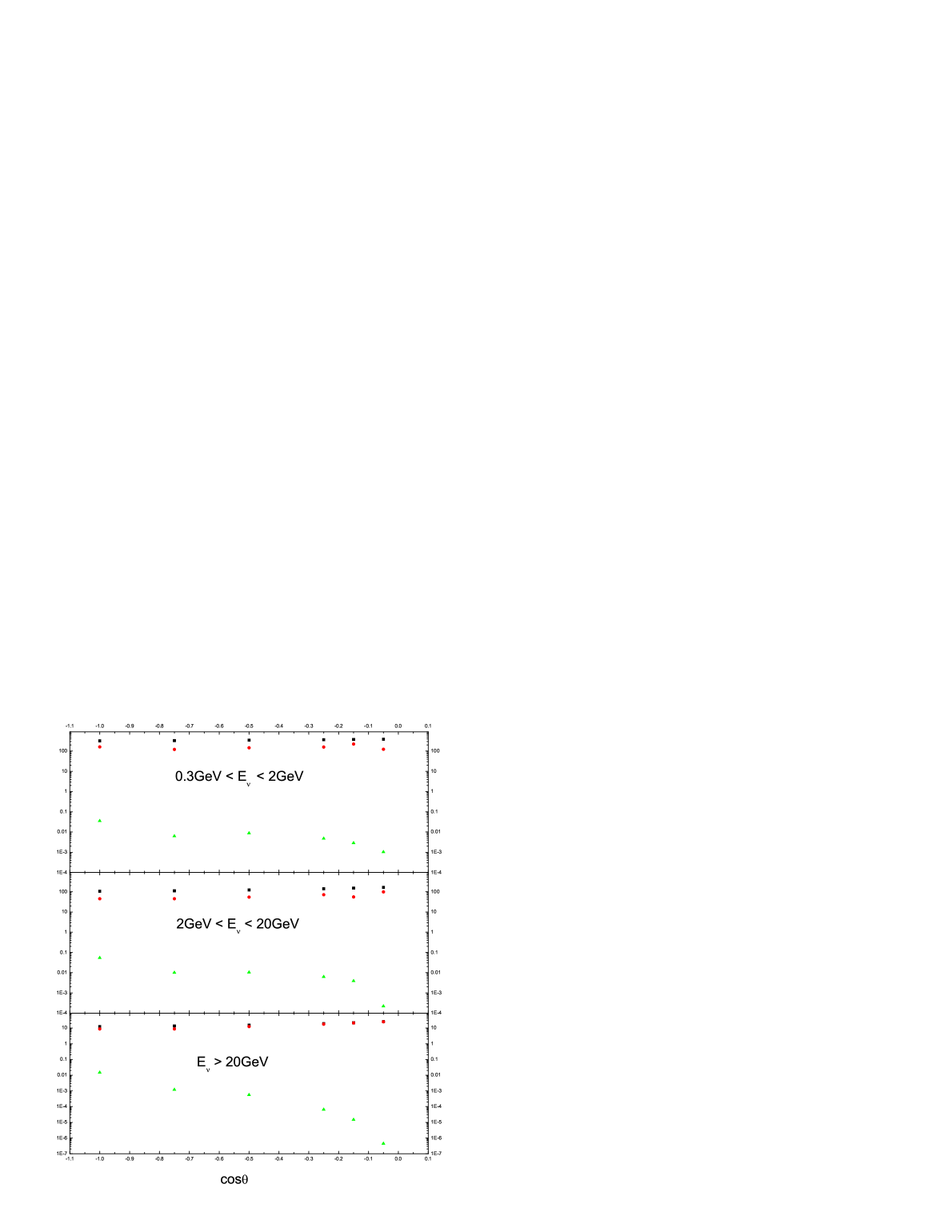
Figure 1: Event numbers plotted as a distribution with zenith angle $\cos\Theta$ in three neutrino energy bins. The square is Hondahonda expectation for no oscillations. The dot is given by substituting $\langle P\rangle$ for $P$ in Eq.(8) and up-triangle represents the variance defined in Eq.(9). These plots use the mass and mixing parameters: $\Delta m^{2}=2.0\times 10^{-3}\textrm{eV}^{2}$, $\sin^{2}2\theta=1.0$, $\sin^{2}\xi=0.19$nakaya , and neutrino travelling distance $L=l-2r\cos\Theta$, where $l$ is the neutrino production height in atmosphere(slant distance in km, listed ingaisser ) and $r=6371\textrm{km}$ is the Earth radius.

In summary, considering that the Earth matter density has uncertainty and this uncertainty has significant effects in some neutrino oscillation cases, such as the $CP$ violation in very long baseline neutrino oscillations and the day-night asymmetry for solar neutrinos, we study this uncertainty in the atmospheric neutrino oscillating scenario of $\nu_{\mu}\rightarrow\nu_{\tau}cos\xi+\nu_{s}sin\xi$, and analyze the effects caused by this uncertainty on the previous fitting results. We find that this uncertainty seems to have no significant effects and need not to modify the previous fitting results fortunately.

Acknowledgment: We thank Lian-Lou Shan, Kerry Whisnant, Bing-Lin Young and Xinmin Zhang for helpful discussions. We also thank Eligio Lisi for kind comments and suggestions. This work is supported partly by the National Natural Science Foundation of China under the Grant No. 90303004.

References

• (1) G.L. Fogli, E. Lisi, and A. Marrone, Phys. Rev. D 63, 053008 (2001).
• (2) S. Fukuda et. al., Phys. Rev. Lett. 85, 3999 (2000); A. Habig, hep-ex/0106025.
• (3) T. Nakaya, hep-ex/0209036.
• (4) L. Wolfenstein, Phys. Rev. D 17, 2369 (1978); S.P. Mikheyev and A.Y. Smirnov, Sov. J. Nucl. Phys. 42, 913 (1985).
• (5) R.J. Geller and T. Hara, Nucl.Instrum.Meth. A503 (2001) 187-191; B. Jacobsson et. al., Phys. Lett. B 532, 259 (2002).
• (6) A.M. Dziewonsky and D.L. Anderson, Phys. Earth Planet. Inter. 25, 297 (1981).
• (7) R. Jeanlow and S. Morris, Annu. Rev. Earth Planet. Sci. 14, 377 (1986); R. Jeanlow, ibid. 18, 357 (1990); F.T. Liu et. al., Geophys. J. Int. 101, 379 (1990); T.P. Yegorova et. al., ibid. 132, 283 (1998); B. Romanowicz, Geophys. Res. Lett. 28, 1107 (2001).
• (8) B.A. Bolt, Q. J. R. Astron. Soc. 32, 367 (1991).
• (9) L.Y. Shan, B.L. Young, and X. Zhang, Phys. Rev. D 66, 053012 (2002).
• (10) L.Y. Shan et. al., Phys. Rev. D 68, 013002 (2003); T. Ohlsson and W. Winter, Phys. Rev. D 68, 073007 (2003).
• (11) L.Y. Shan and X.M. Zhang, Phys. Rev. D 65, 113011 (2002).
• (12) V.D. Barger, T.J. Weiler, and K. Whisnant, Phys. Lett. B 427, 97 (1998); S.C. Gibbons, R.N. Mohapatra, S. Nandi, and A. Raychaudhuri, Phys. Lett. B 430, 296 (1998); N. Gaur, A. Ghosal, E. Ma, and P. Roy, Phys. Rev. D 58, 071301(R) (1998); V. Barger, S. Pakvasa, T.J. Weiler, and K. Whisnant, Phys. Rev. D 58, 093016 (1998).
• (13) A. Tarantola, Inverse Problem Theory, Methods for Data Fitting and Model Parameter Estimation (Elsevier, Amsterdam, 1987).
• (14) M. Honda, T. Kajita, K. Kasahara, and S. Midorikawa, Phys. Rev. D 52, 4985 (1995).
• (15) T.K. Gaisser and T. Stanev, Phys. Rev. D 57, 1977 (1998).