MZ-TH/05-24

Helicity Analysis of Semileptonic Hyperon Decays Including Lepton Mass Effects

A. Kadeer, J. G. Körner and U. Moosbrugger Institut für Physik, Johannes Gutenberg-Universität, D-55099 Mainz , Germany

Abstract

Using the helicity method we derive complete formulas for the joint angular decay distributions occurring in semileptonic hyperon decays including lepton mass and polarization effects. Compared to the traditional covariant calculation the helicity method allows one to organize the calculation of the angular decay distributions in a very compact and efficient way. In the helicity method the angular analysis is of cascade type, i.e. each decay in the decay chain is analyzed in the respective rest system of that particle. Such an approach is ideally suited as input for a Monte Carlo event generation program. As a specific example we take the decay $\Xi^{0}\to\Sigma^{+}+l^{-}+\bar{\nu}_{l}$  ($l^{-}=e^{-},\mu^{-}$) followed by the nonleptonic decay $\Sigma^{+}\to p+\pi^{0}$ for which we show a few examples of decay distributions which are generated from a Monte Carlo program based on the formulas presented in this paper. All the results of this paper are also applicable to the semileptonic and nonleptonic decays of ground state charm and bottom baryons, and to the decays of the top quark.

1 Introduction

Semileptonic hyperon decays have traditionally been analyzed in the rest frame of the decaying parent hyperon using fully covariant methods based on either four-component Dirac spinor methods [1, 2, 3, 4, 5, 6, 7] or on two-component Pauli spinor methods [8, 9, 10]. The latter method is particularly well suited for an implementation of a zero– [8] or a near zero–recoil [9, 10] approximation. In the present paper we employ helicity methods to analyze semileptonic hyperon decays. In the muonic mode it is quite important to incorporate lepton mass effects in the analysis since e.g. in the decay $\Xi^{0}\to\Sigma^{+}+l^{-}+\bar{\nu}_{l}$ the mass difference between the parent and daughter hyperon $M_{\Xi^{0}}-M_{\Sigma^{+}}=(1314.83-1189.37)\,\rm{MeV}=125.46\,{\rm MeV}$ is comparable to the muon mass $m_{\mu}=105.658\,\rm{MeV}$. The analysis proceeds in cascade fashion where every decay in the decay chain is analyzed in its respective rest frame. For the semileptonic decays $\Xi^{0}\to\Sigma^{+}(\to p+\pi^{0})+W^{-}_{\rm{off-shell}}(\to l^{-}+\bar{\nu}_{l})$ $(l=e^{-},\mu^{-})$ treated in this paper this means that the decay $\Xi^{0}\to\Sigma^{+}+W^{-}_{\rm{off-shell}}$ is analyzed in the $\Xi^{0}$ rest frame whereas the decays $\Sigma^{+}\to p+\pi^{0}$ and $W^{-}_{\rm{off-shell}}\to l^{-}+\bar{\nu}_{l}$ are analyzed in the $\Sigma^{+}$ and $W^{-}_{\rm{off-shell}}$ rest frames, respectively. In this way one obtains exact decay formulas with no approximations which are quite compact since they can be written in a quasi–factorized form.

Cascade–type analysis were quite popular some time ago in the strong interaction sector when analyzing the decay chains of the strong interaction baryonic and mesonic resonances (see e.g. [11, 12, 13, 14]). In the weak interaction sector cascade–type analysis were applied before to nonleptonic decays [15, 16, 17, 18, 19, 20, 21, 22], to semileptonic decays of heavy mesons and baryons [17, 18, 19, 23, 24, 25, 26, 27, 28, 29, 30], and to rare decays of heavy mesons [30, 31] and heavy baryons [32]. A new feature appears in semileptonic decays compared to nonleptonic decays when one includes lepton mass effects. In this case one has new interference contributions coming from the time-components of the vector and axial vector currents interfering with the usual three-vector components of the currents (see e.g. [18, 24]).

The results for the angular decay distributions in the semileptonic decays of heavy baryons given e.g. in [18, 28] can in fact be directly transcribed to the hyperon sector . However, the presentation in [18, 28] is rather concise and concentrates on results for angular decay distributions and their analysis rather than presenting the details of their derivations. In order to make the results more reproducible we decided to include the details of the derivations in this paper. This will enable the interested reader to e.g. convert the results of [18], which were derived for the $(l^{+},\nu_{l})$ case, to the $(l^{-},\bar{\nu}_{l})$ case discussed in this paper, or, to derive angular decay formula involving the decay $\Sigma^{+}\to p+\gamma$ instead of the decay $\Sigma^{+}\to p+\pi^{0}$ treated in this paper. At the same time we decided to recalculate all relevant decay formulas in order to provide another independent check of their correctness. In this way we discovered one error in [28] and two errors in [18].

In the simulation of semileptonic hyperon decays including the $\mu$–mode it is important to have a reliable and tested Monte Carlo (MC) program. Since hyperons are produced with nonzero polarization the MC program should also include polarization effects of the decaying parent hyperon. One of the motivations of starting this project was the fact that such a general purpose MC event generator has not been available up to now. Such an event generator should prove to be quite useful in the analysis of the huge amount of data on semileptonic hyperon decays that has been collected by the KTeV and the NA48 collaborations. We wrote and tested such a MC event generator based on the formulas written down in this paper. The present paper can be viewed as a documentation of the theoretical spin-kinematical input that goes into the MC program and, for the sake of reproducibility, the paper also describes how to derive the angular decay distributions entering the MC.

Although we frequently refer to the specific semileptonic cascade decay $\Xi^{0}\to\Sigma^{+}(\to p+\pi^{0})+W^{-}_{\rm{off-shell}}(\to l^{-}+\bar{\nu}_{l})$ the spin–kinematical analysis presented in this paper is quite general and can be equally well applied to the semileptonic decays of heavy charm and bottom baryons, and for that matter, also to the semileptonic decay of the top quark. In order to facilitate such further applications we have always included the necessary sign changes when going from the $(l^{-},\bar{\nu}_{l})$ case to the $(l^{+},\nu_{l})$ case as occurs e.g. in the semileptonic hyperon decay $\Sigma^{+}\to\Lambda+e^{+}+\nu_{e}$, in semileptonic $c\to s$ charm baryon decays or in semileptonic top quark decays [34, 35, 36, 37]. When sign changes are indicated the upper sign will always refer to the $(l^{-},\bar{\nu}_{l})$ case, which is the main concern of this paper, whereas the lower sign will refer to the $(l^{+},\nu_{l})$ case. We also mention that we have always assumed that the amplitudes are relatively real and have therefore dropped azimuthal correlation contributions coming from the imaginary parts. Put in a different language this means that we have not considered $T$–odd contributions in our angular analysis which could result from final state interaction effects or from truly $CP$–violating effects. By keeping the imaginary parts in the azimuthal correlation terms one can easily write down the relevant $T$–odd contributions if needed by using the formulas of this paper. This is discussed for a specific example in Appendix C.

The paper is structured as follows. In Sec. 2 we introduce the helicity amplitudes and relate them to a standard set of invariant form factors. In order to estimate the size of the helicity amplitudes for the $\Xi^{0}\to\Sigma^{+}$ current–induced trasition we provide some simple estimates for the invariant form factors and their $q^{2}$–dependence which we shall refer to as the minimal form factor model. In Sec. 3 we derive the unpolarized decay rate written in terms of bilinear forms of the helicity amplitudes. Sec. 4 contains some numerical results on branching ratios, the rate ratio $\Gamma(e)/\Gamma(\mu)$ and a lepton–side forward-backward asymmetry. In Sec. 5 we discuss single spin polarization effects including spin–momentum correlation effects between the polarization of the parent baryon and the momenta of the decay products. Sec. 6 treats momentum-momentum correlations between the momenta of the decay products in the cascade decay $\Xi^{0}\to\Sigma^{+}(\to p+\pi^{0})+W^{-}_{\rm{off-shell}}(\to l^{-}+\bar{\nu}_{l})$ for an unpolarized $\Xi^{0}$. In Sec. 7 we present a few sample distributions generated from the MC program written by us. Sec. 8 contains our summary and our conclusions.

We have collected some technical material in the appendices. In Appendix A we recount how the two-body decay of a polarized particle is treated in the helicity formalism. This two-body decay enters as a basic building block in our quasi-factorized master formulae in the main text which describe the various cascade–type angular decay distributions presented in this paper. In Appendix B we list explicit forms of the Wigner’s $d^{J}$–function for $J=1/2$ and $J=1$, which are needed in the present application. In Appendix C we go through a specific example and identify a specific $T$–odd term in the joint angular decay distribution written down in Sec. 6. The example is easily generalized to other cases. In Appendix D we finally list the full five–fold angular decay distribution for the cascade decay $\Xi^{0}\to\Sigma^{+}(\to p+\pi^{0})+W^{-}_{\rm{off-shell}}(\to l^{-}+\bar{\nu}_{l})$ for a polarized parent hyperon $\Xi^{0}$. The full five–fold angular decay distribution reduces to the decay distributions listed in the main text after integration or after setting the relevant parameters to zero.

2 The helicity amplitudes

The momenta and masses in the semileptonic hyperon decays are denoted by $B_{1}(p_{1},M_{1})\to B_{2}(p_{2},M_{2})+l(p_{l},m_{l})+\nu_{l}(p_{\nu},0)$. For the hadronic transitions described by the helicity amplitudes it is not necessary to distinguish between the cases $(l^{-},\bar{\nu}_{l})$ and $(l^{+},\nu_{l})$. The matrix elements of the vector and axial vector currents $J_{\mu}^{V,A}$ between the spin $1/2$ states are written as

$$M_{\mu}^{V} =\langle B_{2}|J_{\mu}^{V}|B_{1}\rangle=\bar{u}_{2}(p_{2})\bigg{[}F_{1}^{V}(q^{2})\gamma_{\mu}+\frac{F_{2}^{V}(q^{2})}{M_{1}}\sigma_{\mu\nu}q^{\nu}+\frac{F_{3}^{V}(q^{2})}{M_{1}}q_{\mu}\bigg{]}u_{1}(p_{1})\;,$$ (1)

$$M_{\mu}^{A} =\langle B_{2}|J_{\mu}^{A}|B_{1}\rangle=\bar{u}_{2}(p_{2})\bigg{[}F_{1}^{A}(q^{2})\gamma_{\mu}+\frac{F_{2}^{A}(q^{2})}{M_{1}}\sigma_{\mu\nu}q^{\nu}+\frac{F_{3}^{A}(q^{2})}{M_{1}}q_{\mu}\bigg{]}\gamma_{5}u_{1}(p_{1})\;,$$ (2)

where $q=p_{1}-p_{2}$ is the four–momentum transfer. As in [7] we take $\sigma_{\mu\nu}=\frac{1}{2}(\gamma_{\mu}\gamma_{\nu}-\gamma_{\nu}\gamma_{\mu})$ and $\gamma_{5}=-\left(\begin{array}[]{cc}0&1\\ 1&0\end{array}\right)$. The other $\gamma$ matrices are defined as in Bjorken-Drell.

Next we express the vector and axial vector helicity amplitudes $H_{\lambda_{2}\lambda_{W}}^{V,A}$ $(\lambda_{2}=\pm 1/2$; $\lambda_{W}=t,\pm 1,0$) in terms of the invariant form factors, where $\lambda_{W}$ and $\lambda_{2}$ are the helicity components of the $W_{\rm{off-shell}}$ and the daughter baryon, respectively. Since lepton mass effects are taken into account in this paper we need to retain the time–component “$t$” of the four-currents $J^{V,A}_{\mu}$. Concerning the transformation properties of the four components of the currents one notes that, in the rest frame of the $W_{\rm{off-shell}}$ ($\vec{q}=0$), the three space–components $\lambda_{W}=\pm 1,0$ transform as $J=1$ whereas the time-component transforms as $J=0$. In this paper we use a short–hand notation $\lambda_{W}=t,\pm 1,0$ for $\lambda_{W}=0(J=0);\pm 1,0(J=1)$. Whenever we write $\lambda_{W}=t$ this has to be understood as $\lambda_{W}=0(J=0)$.

One then needs to calculate the expressions

$$H^{V,A}_{\lambda_{2}\lambda_{W}}=M_{\mu}^{V,A}(\lambda_{2})\bar{\epsilon}^{*\mu}(\lambda_{W})\,\,.$$ (3)

We do not explicitly denote the helicity ($m$–quantum number) of the parent hyperon $\lambda_{1}$ in the helicity amplitudes since $\lambda_{1}$ is fixed by the relation $\lambda_{1}=\lambda_{2}-\lambda_{W}$. It is very important to detail the phase conventions when evaluating the expression in Eq. (3). This is because the angular decay distributions to be discussed later on contain interference contributions between different helicity amplitudes which depend on the relative signs of the helicity amplitudes. We shall work in the rest frame of the parent baryon $B_{1}$ with the daughter baryon $B_{2}$ moving in the positive $z$–direction. The baryon spinors are then given by [38]

$$\bar{u}_{2}(\pm{\textstyle\frac{1}{2}},p_{2}) = \sqrt{E_{2}+M_{2}}\left(\chi_{\pm}^{\dagger},\frac{\mp|\vec{p}_{2}|}{E_{2}+M_{2}}\chi_{\pm}^{\dagger}\right)\,,$$

$$u_{1}(\pm{\textstyle\frac{1}{2}},p_{1}) = \sqrt{2M_{1}}\left(\begin{array}[]{c}\chi_{\pm}\\ 0\end{array}\right)\,,$$ (6)

where $\chi_{+}=\left(\begin{array}[]{c}1\\ 0\end{array}\right)$ and $\chi_{-}=\left(\begin{array}[]{c}0\\ 1\end{array}\right)$ are the usual Pauli two-spinors. For the four polarization four-vectors of the currents we have [38]

$$\bar{\epsilon}^{\mu}(t) = \frac{1}{\sqrt{q^{2}}}\left(q_{0};0,0,-p\right)\,,$$

$$\bar{\epsilon}^{\mu}(\pm 1) = \frac{1}{\sqrt{2}}\left(0;\pm 1,-i,0\right)\,,$$

$$\bar{\epsilon}^{\mu}(0) = \frac{1}{\sqrt{q^{2}}}\left(p;0,0,-q_{0}\right)\,,$$ (7)

where $q^{\mu}=(q_{0};0,0,-p)$ is the momentum four–vector of the off–shell gauge boson $W_{\rm{off-shell}}$ in the $B_{1}$ rest frame. The energy of the off-shell $W$–boson $q_{0}$ and the magnitude of three–momentum of the daughter baryon $B_{2}$ (or the off-shell $W$–boson) $p$ in the rest system of the parent baryon $B_{1}$ are given by

$$q_{0} =\frac{1}{2M_{1}}(M_{1}^{2}-M_{2}^{2}+q^{2})\,,$$ (8)

$$p =|\vec{p}_{2}|=\frac{1}{2M_{1}}\sqrt{Q_{+}Q_{-}}\,,$$ (9)

where

$$Q_{\pm}=(M_{1}\pm M_{2})^{2}-q^{2}\,.$$ (10)

The bar over the polarization four-vectors reminds one that the $m$ quantum numbers of the currents are quantized along the negative $z$–direction. They are obtained from the polarization four-vectors quantized along the positive $z$–axis by a $180^{\circ}$ rotation around the $y$–axis (see [38]). Using the spinors in Eq. (2) and the polarization vectors Eq. (2) one obtains following vector helicity amplitudes ($\lambda_{1}=\lambda_{2}-\lambda_{W}$)

$$H_{\frac{1}{2}t}^{V} = \frac{\sqrt{Q_{+}}}{\sqrt{q^{2}}}\bigg{(}(M_{1}-M_{2})F_{1}^{V}+q^{2}/M_{1}F_{3}^{V}\bigg{)}\,,$$

$$H_{\frac{1}{2}1}^{V} = \sqrt{2Q_{-}}\bigg{(}-F_{1}^{V}-(M_{1}+M_{2})/M_{1}F_{2}^{V}\bigg{)}\,,$$

$$H_{\frac{1}{2}0}^{V} = \frac{\sqrt{Q_{-}}}{\sqrt{q^{2}}}\bigg{(}(M_{1}+M_{2})F_{1}^{V}+q^{2}/M_{1}F_{2}^{V}\bigg{)}\,,$$ (11)

and axial vector helicity amplitudes

$$H_{\frac{1}{2}t}^{A} = \frac{\sqrt{Q_{-}}}{\sqrt{q^{2}}}\bigg{(}-(M_{1}+M_{2})F_{1}^{A}+q^{2}/M_{1}F_{3}^{A}\bigg{)}\,,$$

$$H_{\frac{1}{2}1}^{A} = \sqrt{2Q_{+}}\bigg{(}F_{1}^{A}-(M_{1}-M_{2})/M_{1}F_{2}^{A}\bigg{)}\;\,,$$

$$H_{\frac{1}{2}0}^{A} = \frac{\sqrt{Q_{+}}}{\sqrt{q^{2}}}\bigg{(}-(M_{1}-M_{2})F_{1}^{A}+q^{2}/M_{1}F_{2}^{A}\bigg{)}\,.$$ (12)

From parity or from an explicit calculation one has

$$H_{-\lambda_{2},-\lambda_{W}}^{V} = H_{\lambda_{2},\lambda_{W}}^{V}\,$$

$$H_{-\lambda_{2},-\lambda_{W}}^{A} = -H_{\lambda_{2},\lambda_{W}}^{A}$$ (13)

When discussing the semileptonic transitions close to the zero recoil point it is advantageous to make use of the velocity transfer variable $\omega=v_{1}\cdot v_{2}$ where $v^{\mu}=p^{\mu}/M$. The velocity transfer variable can be expressed in terms of the usual momentum transfer variable $q^{2}$. One has

$$\omega=(M_{1}^{2}+M_{2}^{2}-q^{2})/(2M_{1}M_{2})\,,$$ (14)

or

$$q^{2}=(M_{1}-M_{2})^{2}-2M_{1}M_{2}(\omega-1)\,\,.$$ (15)

The maximal and minimal values of the velocity transfer variable $\omega$ are $\omega_{\rm{max}}=(M_{1}^{2}+M_{2}^{2}-m_{l}^{2})/(2M_{1}M_{2})$ and $\omega_{\rm{min}}=1$, respectively. The minimal value $\omega_{\rm{min}}=1$ is referred to as the zero recoil point since this is the point where the recoiling daughter baryon has no three–momentum. For the variables $Q_{\pm}$ defined in Sec. 2 one finds $Q_{\pm}=2M_{1}M_{2}(\omega\pm 1)$ which gives $p=M_{2}\sqrt{\omega^{2}-1}$ where $p$ is the momentum of the recoiling daughter baryon. The relevant expansion parameter close to the zero recoil point is thus $\sqrt{\omega-1}$. For example, at the zero recoil point only the helicity amplitudes $H_{\frac{1}{2}t}^{V}$ (allowed Fermi transition) and $H_{\frac{1}{2}0}^{A}=-H_{\frac{1}{2}1}^{A}/\sqrt{2}$ (allowed Gamov–Teller transition) survive. In the LS–coupling scheme with LS–amplitudes $T_{LS}$, these correspond to the $S$–wave transition amplitudes $T^{V}_{0\frac{1}{2}}$ and $T^{A}_{0\frac{1}{2}}$, respectively, where the orbital angular momentum $L$ is defined with respect to the relative orbital motion of the baryon $B_{2}$ and the $W^{-}_{\rm{off-shell}}$ in the rest frame of the baryon $B_{1}$. In the literature one can find very ingenious approximation formulae for various decay distributions and polarization observables which are based on a near zero recoil expansion [9, 10]. These are usually referred to as effective theories of semileptonic hyperon decays. In this paper we shall, however, not discuss zero recoil or near zero recoil approximations but we always retain the full structure of the physical observables without any approximations.

In order to get a feeling about the size of the helicity amplitudes we make a simple minimal ansatz for the invariant amplitudes at zero momentum transfer using $SU(3)$ symmetry. The analysis is greatly simplified by the fact that the C.G. coefficients for the $(n\to p)$–transition are the same as those for the $(\Xi^{0}\to\Sigma^{+})$–transition. One thus has $F_{1}^{V}(0)=1$ and $F_{1}^{A}(0)=1.267$ where the vector form factor $F_{1}^{V}(0)$ is protected from first order symmetry breaking effects by the Ademollo-Gatto theorem [39, 40]. For the magnetic form factor $F_{2}^{V}(0)$ we take $F_{2}^{V}(0)=M_{\Xi^{0}}(\mu_{p}-\mu_{n})/(2M_{p})=2.6$ as in [7], where $\mu_{p}$ and $\mu_{n}$ are the anomalous magnetic moments of the proton and neutron. The second class current contributions are set to zero, i.e. we take $F_{3}^{V}(0)=F_{2}^{A}(0)=0$. Note that a first class quark current can in principle populate the second class form factors $F_{3}^{V}$ and $F_{2}^{A}$ when $M_{1}\neq M_{2}$. For example, in the covariant spectator quark model calculation of [44, 45] one finds $F_{3}^{V}(0)=(M_{1}-M_{2})/(6M_{2})=0.0176$ and $F_{2}^{A}(0)=0$. However, since we are not including $SU(3)$ symmetry breaking effects for the other form factors we set $F_{3}^{V}$ and $F_{2}^{A}$ to zero for consistency reasons since they vanish in the $SU(3)$ symmetry limit. For $F_{3}^{A}(0)$ we use the Goldberger-Treiman relation $F_{3}^{A}(0)=M_{\Xi^{0}}(M_{\Xi^{0}}+M_{\Sigma^{+}})F_{1}^{A}(0)/(m_{K^{-}})^{2}=17.1$ (see e.g. [41]).

For the $q^{2}$–dependence of the invariant form factors we take a Veneziano–type ansatz which has given a good description of the $q^{2}$–dependence of the electromagnetic form factors of the neutron and proton [46]. We write

$$F_{i}^{V,A}(q^{2}) =F_{i}^{V,A}(0)\prod_{n=0}^{n_{i}}\frac{1}{1-\frac{q^{2}}{m_{V,A}^{2}+n\alpha^{{}^{\prime}-1}}}\approx F_{i}^{V,A}(0)\left(1+q^{2}\sum_{n=0}^{n_{i}}\frac{1}{m_{V,A}^{2}+n\alpha^{{}^{\prime}-1}}\right)\,.$$ (16)

For $F_{1}^{V}(q^{2})$ and $F_{2}^{V}(q^{2})$ we use $m_{V}=m_{K^{*}(892)}=0.892$ GeV which is the lowest lying strange vector meson with $J^{P}=1^{-}$ quantum numbers. Correspondingly we use $m_{A}=m_{K^{*}(1.270)}=1.273\,{\rm GeV}$ ($J^{P}=1^{+}$) for $F_{1}^{A}(q^{2})$ and $m_{A}=m_{K}=0.494\,{\rm GeV}$ ($J^{P}=0^{-}$) for $F_{3}^{A}(q^{2})$, respectively. The slope of the Regge trajectory is taken as $\alpha^{\prime}=0.9\,{\rm GeV}^{-2}$. The number of poles in Eq. (16) is determined by the large $q^{2}$ power counting laws. One thus has $n_{1}=1$ and $n_{2,3}=2$. For the slopes of the form factors we thus have 1.781, 2.113, 0.983 and 5.241 $\rm{GeV}^{-2}$ for $F_{1}^{V},F_{2}^{V},F_{1}^{A}$ and $F_{3}^{A}$, respectively. These values correspond to (“charge”) radii $\langle r^{2}\rangle$ of 0.416, 0.494, 0.230 and 1.224 ${\rm fm}^{2}$, respectively, for the four above form factors. The (“charge”) radii of the $F_{1}^{V}$ and $F_{1}^{A}$ form factors are close to the radii calculated in [47] using chiral input and a relativistic constituent quark model. The $q^{2}$–dependence of the form factors introduces only small effects since the range of $q^{2}$ is so small for the $\Xi^{0}\to\Sigma^{+}$ transitions. For the largest $q^{2}$–value $q^{2}_{\rm{max}}=(M_{1}-M_{2})^{2}$, the form factors have only increased by $2.8\%\,(F_{1}^{V})$, $3.3\%\,(F_{2}^{V})$, $1.5\%\,(F_{1}^{A})$ and $8.2\%\,(F_{3}^{A})$ from their $q^{2}=0$ values.

Based on these estimates for the invariant form factors we show in Fig. 1 a plot of the $q^{2}$–dependence of the six helicity amplitudes. For easier comparability we have plotted the quantities $\sqrt{q^{2}}H_{\lambda_{2}\lambda_{W}}^{V,A}$. Close to the lower boundary $q^{2}=m_{e}^{2}$ the longitudinal and scalar helicity amplitudes dominate, with $H_{\frac{1}{2}0}^{V}\approx H_{\frac{1}{2}t}^{V}$ and $H_{\frac{1}{2}0}^{A}\approx H_{\frac{1}{2}t}^{A}$. Close to the upper boundary at the zero recoil point $q^{2}=(M_{1}-M_{2})^{2}$, which is the relevant region for the $\mu$–mode, the orbital $S$–wave contributions $H_{\frac{1}{2}t}^{V}$ and $H_{\frac{1}{2}1}^{A}=-\sqrt{2}H_{\frac{1}{2}0}^{A}$ are the dominant amplitudes with $H_{\frac{1}{2}t}^{V}=-(F_{1}^{V}/F_{1}^{A})H_{\frac{1}{2}0}^{A}$ when $F_{3}^{V}=F_{2}^{A}=0$.

Figure 1: The $q^{2}$–dependence of the six independent helicity amplitudes $S(V,A):=\sqrt{q^{2}}H_{\frac{1}{2}t}^{V,A},\,T(V,A):=\sqrt{q^{2}}H_{\frac{1}{2}1}^{V,A}$ and $L(V,A):=\sqrt{q^{2}}H_{\frac{1}{2}0}^{V,A}$ multiplied by $\sqrt{q^{2}}$ for the $e$-mode (full range) and for the $\mu$–mode (to the right of the vertical line $q^{2}=m_{\mu}^{2}$). We also display the corresponding helicity amplitudes with the contributions of $F_{2}^{V}(q^{2})$ and $F_{3}^{A}(q^{2})$ switched off (dashed lines).

In Fig. 1 we also show plots of the helicity amplitudes where the contributions of the form factors $F_{2}^{V}(q^{2})$ and $F_{3}^{A}(q^{2})$ have been switched off. The difference is not discernible at the scale of the plot for the helicity form factors $H_{\frac{1}{2}0}^{V}$, $H_{\frac{1}{2}t}^{V}$, $H_{\frac{1}{2}1}^{A}$ and $H_{\frac{1}{2}0}^{A}$ and is small for $H_{\frac{1}{2}t}^{A}$. The difference is, however, sizeable for $H_{\frac{1}{2}1}^{V}$. This can be understood from Eq. (2) which shows that, even though $H_{\frac{1}{2}1}^{V}$ is small because it is proportional to $\sqrt{Q_{-}}$ and thus of overall order $O((M_{1}-M_{2})/M_{1})$, the relative contribution of $F_{2}^{V}$ to $H_{\frac{1}{2}1}^{V}$ is not suppressed by a factor of $O((M_{1}-M_{2})/M_{1})$ as it is in the other helicity form factors. Thus a measurement of the helicity form factor $H_{\frac{1}{2}1}^{V}$ would be ideally suited to determine the strength of $F_{2}^{V}$. In fact, in Sec. 4 we shall discuss a forward-backward asymmetry measure which is proportional to $H_{\frac{1}{2}1}^{V}$ and is thus well suited for a measurement of $F_{2}^{V}$.

We caution the reader that our ansatz for the form factors is only meant to implement the gross features of the dynamics of the semileptonic hyperon decays $\Xi^{0}\to\Sigma^{+}+l^{-}+\bar{\nu}_{l}$ which will eventually be superseded by the results of a careful analysis of the decay data. We shall nevertheless use the above minimal model for the $\Xi^{0}\to\Sigma^{+}$ form factors to calculate branching rates, the rate ratio $\Gamma(e)/\Gamma(\mu)$ and a forward-backward asymmetry in Sec. 4, the longitudinal and transverse polarizations of the daughter baryon and the lepton in Sec. 5 and a mean azimuthal correlation parameter in Sec. 6 for this decay. In Sec. 7 we also show some Monte Carlo plots which are again based on the minimal form factor model.

In the subsequent sections the rate and the angular decay distributions will mostly be written in terms of bilinear products of the sum of the vector and axial vector helicity amplitudes

$$H_{\lambda_{2}\lambda_{W}}=H_{\lambda_{2}\lambda_{W}}^{V}+H_{\lambda_{2}\lambda_{W}}^{A}\,,$$ (17)

since it is this combination which appears naturally in the master formulas describing the rate and the various decay distributions. One can of course rewrite the rate and the decay distributions in terms of bilinear products of the vector and axial vector helicity amplitudes $H_{\lambda_{2}\lambda_{W}}^{V}$ and $H_{\lambda_{2}\lambda_{W}}^{A}$. For the decay distributions this can be quite illuminating if one wishes to identify the overall parity nature of the observables that multiply the angular terms in the angular decay distributions.

3 Unpolarized decay rate

The differential decay rate is given by (see e.g. [24])

$$\frac{d\Gamma}{dq^{2}dE_{l}}=\frac{G_{F}^{2}}{(2\pi)^{3}}|V_{us}|^{2}\frac{1}{8M_{1}^{2}}L_{\mu\nu}H^{\mu\nu}\;,$$ (18)

where $L_{\mu\nu}$ is the usual lepton tensor ($\varepsilon_{0123}=+1$)

$$L^{\mu\nu}=p_{l}^{\mu}p_{\nu}^{\nu}+p_{l}^{\nu}p_{\nu}^{\mu}-\frac{q^{2}-m_{l}^{2}}{2}g^{\mu\nu}\pm i\varepsilon^{\mu\nu\alpha\beta}p_{l,\alpha}p_{\nu,\beta}\,\,.$$ (19)

As stated in the introduction the upper sign refers to the $(l^{-},\bar{\nu}_{l})$ case, whereas the lower sign refers to the $(l^{+},\nu_{l})$ case.

The hadron tensor $H_{\mu\nu}$ is given by the tensor product of the vector and axial vector matrix elements defined in Eqs. (1) and (2), cf.

$$H_{\mu\nu}=(M^{V}+M^{A})_{\mu}\,\,(M^{V}+M^{A})_{\nu}^{\dagger}\,\,.$$ (20)

Eq. (18) shows that $L_{\mu\nu}H^{\mu\nu}$ determines the dynamical weight function in the $(q^{2},E_{l})$ Dalitz plot (see e.g. the discussion in [43]). In a Monte Carlo generator one would thus have to generate events according to the weight $L_{\mu\nu}H^{\mu\nu}$ in the $(q^{2},E_{l})$ Dalitz plot.

The differential $q^{2}$–distribution can be obtained from Eq. (18) by $E_{l}$–integration, where the limits are given by (see e.g. [24])

$$E_{l}^{\pm}=\frac{1}{2q^{2}}\Big{(}q_{0}(q^{2}+m_{l}^{2})\pm p(q^{2}-m_{l}^{2})\Big{)}.$$ (21)

Finally, in order to get the total rate one has to integrate over $q^{2}$ in the limits $m_{l}^{2}\leqslant q^{2}\leqslant(M_{1}-M_{2})^{2}$.

On reversing the order of integrations, the differential lepton energy distribution can be obtained from Eq. (18) by $q^{2}$–integration. The relevant integration limits can be obtained from the inverse of Eq. (21). One obtains (see e.g. [24])

$$q^{2}_{\pm}=\frac{1}{a}(b\pm\sqrt{b^{2}-ac})\,\,,$$ (22)

where

$$a = M_{1}^{2}+m_{l}^{2}-2M_{1}E_{l}\,,$$

$$b = M_{1}E_{l}(M_{1}^{2}-M_{2}^{2}+m_{l}^{2}-2M_{1}E_{l})+m_{l}^{2}M_{2}^{2}\,,$$

$$c = m_{l}^{2}\Big{(}(M_{1}^{2}-M_{2}^{2})^{2}+m_{l}^{2}M_{1}^{2}-(M_{1}^{2}-M_{2}^{2})2M_{1}E_{l}\Big{)}\,.$$

Using $E_{l}({\rm max}):=E_{{\rm max}}=(M_{1}^{2}-M_{2}^{2}+m_{l}^{2})/(2M_{1})$ and $E_{l}({\rm min}):=E_{{\rm min}}=m_{l}$ one can simplify Eq. (22) to write

$$q^{2}_{\pm} =\frac{2M_{1}^{2}}{2M_{1}(E_{\rm{max}}-E_{l})+M_{2}^{2}}\bigg{(}(E_{\rm{max}}-E_{l})\Big{(}E_{l}\pm\sqrt{E_{l}^{2}-E_{\rm{min}}^{2}}\,\,\Big{)}+\frac{m_{l}^{2}M_{2}^{2}}{2M_{1}^{2}}\bigg{)}.$$ (23)

Finally, in order to get the total rate, one has to integrate over the lepton energy in the limits $m_{l}\leqslant E_{l}\leqslant(M_{1}^{2}-M_{2}^{2}+m_{l}^{2})/2M_{1}$.

As it turns out the two–dimensional integration becomes much simpler if one considers the two–fold differential rate with respect to the variables $q^{2}$ and $\cos\theta$ instead, where $\theta$ is the polar angle of the lepton in the $(l,\nu_{l})$ c.m. system relative to the momentum direction of the $W_{\rm{off-shell}}$. $E_{l}$ and $\cos\theta$ are related by (see e.g. [24])

$$\cos\theta=\frac{2q^{2}E_{l}-q_{0}(q^{2}+m_{l}^{2})}{p(q^{2}-m_{l}^{2})}\,.$$ (24)

Differentiating Eq. (24) one has

$$\frac{d\cos\theta}{dE_{l}}=\frac{2q^{2}}{p(q^{2}-m_{l}^{2})}\,,$$ (25)

which leads to the differential decay distribution

$$\frac{d\Gamma}{dq^{2}d\cos\theta}=\frac{G_{F}^{2}}{(2\pi)^{3}}|V_{us}|^{2}\frac{(q^{2}-m_{l}^{2})p}{16M_{1}^{2}q^{2}}L_{\mu\nu}H^{\mu\nu}\;.$$ (26)

It is clear from comparing Eqs. (18) and (26) that, when writing a Monte Carlo program, one should not generate events in the ($q^{2},\cos\theta$) Dalitz plot according to the weight $L_{\mu\nu}H^{\mu\nu}$.

The $\cos\theta$ dependence of $L_{\mu\nu}H^{\mu\nu}$ can be easily worked out by following the methods described in [24] which is based on the completeness relation for the polarization four–vectors

$$\sum_{m,m^{\prime}=t,\pm,0}\bar{\epsilon}^{\mu}(m)\bar{\epsilon}^{*\nu}(m^{\prime})g_{mm^{\prime}}=g^{\mu\nu}\,.$$ (27)

The tensor $g_{mm^{\prime}}=\mbox{diag}(+,-,-,-)$ is the spherical representation of the metric tensor where the components are ordered in the sequence $m,m^{\prime}=t,\pm 1,0$. One can then rewrite the contraction of the lepton and hadron tensors $L_{\mu\nu}H^{\mu\nu}$ as

$$L_{\mu\nu}H^{\mu\nu} =L^{\mu^{\prime}\nu^{\prime}}g_{\mu^{\prime}\mu}g_{\nu^{\prime}\nu}H^{\mu\nu}=\sum_{m,m^{\prime},n,n^{\prime}}L^{\mu^{\prime}\nu^{\prime}}\bar{\epsilon}_{\mu^{\prime}}(m)\bar{\epsilon}_{\mu}^{*}(m^{\prime})g_{mm^{\prime}}\bar{\epsilon}_{\nu^{\prime}}^{*}(n)\bar{\epsilon}_{\nu}(n^{\prime})g_{nn^{\prime}}H^{\mu\nu}$$

$$=\sum_{m,m^{\prime},n,n^{\prime}}\bigg{(}L^{\mu^{\prime}\nu^{\prime}}\bar{\epsilon}_{\mu^{\prime}}(m)\bar{\epsilon}_{\nu^{\prime}}^{*}(n)\bigg{)}\bigg{(}H^{\mu\nu}\bar{\epsilon}_{\mu}^{*}(m^{\prime})\bar{\epsilon}_{\nu}(n^{\prime})\bigg{)}\,g_{mm^{\prime}}g_{nn^{\prime}}\,\,.$$ (28)

We shall refer to the second and third lines of Eq. (3) as the semi-covariant representation of the angular decay distribution.

One has to remember that Eq. (3) refers to the differential rate of the decay of an unpolarized parent hyperon into a daughter baryon whose spin is not observed. This means that one has to take into account the additional conditions $\lambda_{1}=\lambda^{\prime}_{1}$ and $\lambda_{2}=\lambda^{\prime}_{2}$ in Eq. (3). Angular momentum conservation then implies that not all index pairs $m=m^{\prime}$ and $n=n^{\prime}$ in Eq. (3) can be realized. Taking angular momentum conservation into account one has diagonal contributions $m=m^{\prime}=n=n^{\prime}=t,\pm 1,0$ as well as nondiagonal contributions with $m=m^{\prime}=t$ and $n=n^{\prime}=0$ and vice versa.

The point of writing $L_{\mu\nu}H^{\mu\nu}$ in the factorized form of Eq. (3) is that each of the two factors in the second line of Eq. (3) is Lorentz invariant and can thus be evaluated in different Lorentz frames. The leptonic part will be evaluated in the $(l,\nu_{l})$ center–of–mass (c.m.) frame (or $W_{\rm{off-shell}}$–rest frame) bringing in the decay angle $\theta$, whereas the hadronic part will be evaluated in the $\Xi^{-}$ rest frame bringing in the helicity amplitudes defined in Sec. 2.

Turning to the $(l,\nu_{l})$ c.m system the lepton momenta in the $(x,y,z)$–system read (see Fig. 3)

$$p_{l}^{\mu} = (E_{l}\,;p_{l}\sin\theta,0,-p_{l}\cos\theta)\,,$$ (29)

$$p_{\nu}^{\mu} = p_{l}\,(1,-\sin\theta,0,\cos\theta)\,.$$

The angle $\theta$ is always measured with respect to the direction of the lepton $l$, regardless of whether we are dealing with the $(l^{-},\bar{\nu}_{l})$ or the $(l^{+},\nu_{l})$ case. Since the orientation in the $(x,y)$–plane need not be specified in the present problem we have chosen the lepton momenta to lie in the $(x,z)$–plane. $E_{l}$ and $p_{l}$ are the energy and the magnitude of the three-momentum of the charged lepton in the $(l,\nu_{l})$ c.m system, respectively, given by $E_{l}=(q^{2}+m_{l}^{2})/2\sqrt{q^{2}}$ and $p_{l}=(q^{2}-m_{l}^{2})/2\sqrt{q^{2}}$. The longitudinal and time-component polarization four–vectors take the form $\bar{\epsilon}^{\mu}(0)=(0;0,0,-1)$ and $\bar{\epsilon}^{\mu}(t)=(1;0,0,0)$ whereas the transverse parts are unchanged from Eq. (2). Using the explicit form of the lepton tensor Eq. (19) it is then not difficult to evaluate Eq. (3) in terms of the helicity amplitudes $H_{\lambda_{2}\lambda_{W}}$ of Sec. 2. One obtains

$$L_{\mu\nu}H^{\mu\nu} = \frac{2}{3}(q^{2}-m_{l}^{2})\;\bigg{[}\frac{3}{8}(1\mp\cos\theta)^{2}|H_{\frac{1}{2}1}|^{2}+\frac{3}{8}(1\pm\cos\theta)^{2}|H_{-\frac{1}{2}-1}|^{2}$$ (30)

$$+\;\frac{3}{4}\sin^{2}\theta(|H_{\frac{1}{2}0}|^{2}+|H_{-\frac{1}{2}0}|^{2})$$

$$+\;\frac{m_{l}^{2}}{2q^{2}}\;\Big{\{}\frac{3}{2}(|H_{\frac{1}{2}t}|^{2}+|H_{-\frac{1}{2}t}|^{2})+\frac{3}{4}(|H_{\frac{1}{2}1}|^{2}+|H_{-\frac{1}{2}-1}|^{2})\sin^{2}\theta$$

$$+\;\frac{3}{2}\cos^{2}\theta(|H_{\frac{1}{2}0}|^{2}+|H_{-\frac{1}{2}0}|^{2})-3\cos\theta(H_{\frac{1}{2}t}H_{\frac{1}{2}0}+H_{-\frac{1}{2}t}H_{-\frac{1}{2}0})\Big{\}}\;\bigg{]}\;,$$

where the $H_{\lambda_{2}\lambda_{W}}$ are the sums of the corresponding vector and axial vector helicity amplitudes defined in Eq. (17). We mention that the helicity flip factor $m_{l}/2q^{2}$ does not give rise to a singularity since $q^{2}\geq m_{l}^{2}$.

By explicit verification, or by hindsight, one can show that Eq. (3) can be written very compactly in terms of Wigner’s $d^{J}$–functions. One has what we shall refer to as our first master formula

$$L_{\mu\nu}H^{\mu\nu}= \frac{1}{8}\sum_{\lambda_{l},\lambda_{2},\lambda_{W},\lambda^{\prime}_{W},J,J^{\prime}}(-1)^{J+J^{\prime}}|h^{l}_{\lambda_{l}\lambda_{\nu}=\pm\frac{1}{2}}|^{2}\times$$

$$\times\delta_{\lambda_{2}-\lambda_{W},\lambda_{2}-\lambda^{\prime}_{W}}d_{\lambda_{W},\lambda_{l}\mp\frac{1}{2}}^{J}(\theta)d_{\lambda^{\prime}_{W},\lambda_{l}\mp\frac{1}{2}}^{J^{\prime}}(\theta)H_{\lambda_{2}\lambda_{W}}H_{\lambda_{2}\lambda^{\prime}_{W}}^{\ast}\;.$$ (31)

Except for the phase factor $(-1)^{J+J^{\prime}}$ the master formula can in fact be derived by repeated application of the basic two–body decay formula in Appendix A. The Kronecker $\delta$-function $\delta_{\lambda_{2}-\lambda_{W},\lambda_{2}-\lambda^{\prime}_{W}}$ in Eq. (3) expresses the fact that we are dealing with the decay of an unpolarized parent hyperon. One has to remember that $\lambda_{W}=0$ and $\lambda_{W}=t$ both refer to the helicity projection 0 (see Sec. 2). Therefore there are nondiagonal interference contributions between $J=1,\lambda_{W}=0$ and $J=0,\lambda_{W}=t$ because they are allowed by the angular momentum conservation condition $\lambda_{2}-\lambda_{W}=\lambda_{2}-\lambda^{\prime}_{W}$ implying $\lambda_{W}=\lambda^{\prime}_{W}$. The interference contributions carry an extra minus sign as can be seen from the phase factor $(-1)^{J+J^{\prime}}$ in Eq. (3). The phase factor $(-1)^{J+J^{\prime}}$ comes in because of the pseudo–Euclidean nature of the spherical metric tensor $g_{mm^{\prime}}$ defined after Eq. (27).

The sign change in the first line of Eq. (30) going from the $(l^{-},\bar{\nu}_{l})$ to the $(l^{+},\nu_{l})$ case can now be seen to result from the products of the relevant elements of the Wigner’s $d^{1}$–functions. For example, for $\lambda_{2}=1/2$, $\lambda_{W}=1$ the nonflip contributions $(\lambda_{l}=-\lambda_{\nu}=\mp 1/2)$ are proportional to $(d^{1}_{1,\mp 1})^{2}=({\textstyle\frac{1}{2}}(1\mp\cos\theta))^{2}$. There are no corresponding sign changes in the other lines of Eq. (30).

The $h_{\lambda_{l}\lambda_{\nu}}$ are the helicity amplitudes of the final lepton pair in the $(l,\nu)$ c.m. system. For example, for the $(l^{-},\bar{\nu})$ case with $\vec{p}_{l^{-}}$ along the positive $z$-axis, they can be worked out by using Eq. (2), the negative energy spinor of the massless antineutrino with helicity $\lambda_{\bar{\nu}}=\frac{1}{2}$ given by

$$v_{\bar{\nu}}({\textstyle\frac{1}{2}})=\sqrt{E_{\nu}}\left(\begin{array}[]{c}\chi_{+}\\ -\chi_{+}\end{array}\right)\,,$$ (32)

and the SM form of the lepton current ($\lambda_{W}=\lambda_{l^{-}}-\lambda_{\bar{\nu}}$)

$$h_{\lambda_{l^{-}}=\mp\frac{1}{2},\lambda_{\bar{\nu}}=\frac{1}{2}}=\bar{u}_{l^{-}}(\mp{\textstyle\frac{1}{2}})\gamma^{\mu}(1+\gamma_{5})v_{\bar{\nu}}({\textstyle\frac{1}{2}})\left\{{\epsilon_{\mu}(-1)\atop\epsilon_{\mu}(t),\epsilon_{\mu}(0)}\right\}\,.$$ (33)

We shall refer to the upper case $\lambda_{l^{-}}=-\frac{1}{2}$ as the nonflip transition and to the lower case $\lambda_{l^{-}}=\frac{1}{2}$ as the flip transition. Note the unconventional form of the SM lepton current which is due to the $\gamma_{5}$ definition in Sec. 2. The polarization four–vectors are given by $\epsilon^{\mu}(t)=(1;0,0,0)$, $\epsilon^{\mu}(0)=(0;0,0,1)$ and $\epsilon^{\mu}(\pm 1)=(0;\mp 1,-i,0)/\sqrt{2}$. The flip contribution is identical for $\lambda_{W}=t$ and $\lambda_{W}=0$. A similar expression can be written down for the case $(l^{+},\nu_{l})$ which we shall not work out in explicit form. For the moduli squared of the helicity amplitudes one finally obtains

$$\rm{nonflip}\,\,(\lambda_{W}=\mp 1):|h_{\lambda_{l}=\mp\frac{1}{2},\lambda_{\nu}=\pm\frac{1}{2}}|^{2} =8(q^{2}-m_{l}^{2})\;,$$ (34)

$$\rm{flip}\,\,(\lambda_{W}=t,0):|h_{\lambda_{l}=\pm\frac{1}{2},\lambda_{\nu}=\pm\frac{1}{2}}|^{2} =8\frac{m_{l}^{2}}{2q^{2}}(q^{2}-m_{l}^{2})\;.$$ (35)

The notation in Eqs.(34) and (35) (and elsewhere in the paper) is such that the upper and lower signs refer to the configurations $(l^{-},\bar{\nu}_{l})$ and $(l^{+},\nu_{l})$, respectively. In Eq. (3) the sum over $J,J^{\prime}$ runs over $0$ and $1$ and the index $\lambda_{W},\lambda^{\prime}_{W}$ runs over the four components $t,\pm 1,0$. As remarked on before one has to remember to include the interference contribution from $(J=0;\lambda_{W}=t)$ and $(J=1;\lambda_{W}=0)$ giving an extra minus sign. The matrix $d^{1}_{mm^{\prime}}$, finally, is Wigner’s $d^{1}$–function ($d^{0}_{mm^{\prime}}=1$ for $m,m^{\prime}=t$) listed in Appendix B.

The form Eq. (3) readily affords a physical interpretation. $H_{\lambda_{2}\lambda_{W}}H_{\lambda_{2}\lambda^{\prime}_{W}}^{\ast}$ determines the density matrix of the $W_{\rm{off-shell}}$ (which happens to be block-diagonal in the present application). The density matrix is then “rotated” into the direction of the lepton in the $(l,\nu_{l})$ c.m. system with the help of the $d^{1}$–functions whence the squared helicity amplitudes $|h_{\lambda_{l}\lambda_{\nu}}|^{2}$ determine the helicity dependent rates into the lepton pair.

Performing the sum in Eq. (3) $(\lambda_{l}=\pm 1/2;\lambda_{W}=t,\pm 1,0;J=0,1;J^{\prime}=0,1;\lambda_{2}=\pm 1/2)$ one recalculates Eq. (30). Note that the flip contribution proportional to $m_{l}^{2}/2q^{2}$ and nonflip contributions are clearly separated in Eq. (30). This separation facilitates the determination of the longitudinal polarization of the lepton to be discussed in Sec. 5.

The differential rate $d\Gamma/dq^{2}$ is obtained from Eqs. (26) and (30) by $\cos\theta$–integration which, in a sense, is trivial. One obtains

$$\frac{d\Gamma}{dq^{2}}= \frac{1}{3}\frac{G_{F}^{2}}{(2\pi)^{3}}|V_{us}|^{2}\frac{(q^{2}-m_{l}^{2})^{2}p}{8M_{1}^{2}q^{2}}\bigg{[}|H_{\frac{1}{2}1}|^{2}+|H_{-\frac{1}{2}-1}|^{2}+|H_{\frac{1}{2}0}|^{2}+|H_{-\frac{1}{2}0}|^{2}$$

$$+\;\frac{m_{l}^{2}}{2q^{2}}\;\Big{\{}3\Big{(}\,|H_{\frac{1}{2}t}|^{2}+|H_{-\frac{1}{2}t}|^{2}\,\Big{)}+|H_{\frac{1}{2}1}|^{2}+|H_{-\frac{1}{2}-1}|^{2}+\;|H_{\frac{1}{2}0}|^{2}+|H_{-\frac{1}{2}0}|^{2}\Big{\}}\;\bigg{]}\;.$$ (36)

The remaining $q^{2}$–integration ($m_{l}^{2}\leqslant q^{2}\leqslant(M_{1}-M_{2})^{2}$) has to be done numerically because of the nontrivial $q^{2}$–dependence of the invariant form factors.

A check on Eq. (3) is afforded by recalculating the Standard Model (SM) formula for semileptonic free quark decay $q_{1}\to q_{2}+l+\nu$ setting $F_{1}^{V}(q^{2})=F_{1}^{A}(q^{2})=1$ and $F_{2,3}^{V,A}=0$ in Eq. (3). One obtains

$$\frac{d\Gamma^{SM}}{d\hat{q}^{2}} =\Gamma_{0}\frac{(\hat{q}^{2}-\eta^{2})^{2}}{\hat{q}^{4}}4\hat{p}\bigg{(}-2\hat{q}^{4}+\hat{q}^{2}(1+\rho^{2})+(1-\rho^{2})^{2}$$

$$\quad+\frac{\eta^{2}}{2\hat{q}^{2}}\Big{\{}-2\hat{q}^{4}-2\hat{q}^{2}(1+\rho^{2})+4(1-\rho^{2})^{2}\Big{\}}\bigg{)}\,,$$ (37)

where we have introduced scaled variables according to $\hat{p}=p/M_{1}$, $\hat{q}^{2}=q^{2}/M_{1}^{2}$, $\rho^{2}=M_{2}^{2}/M_{1}^{2}$ and $\eta^{2}=m_{l}^{2}/M_{1}^{2}$, and where $\hat{p}=\frac{1}{2}(1+\rho^{4}+\hat{q}^{4}-2\rho^{2}-2\hat{q}^{2}-2\rho^{2}\hat{q}^{2})^{1/2}$ is the scaled magnitude of the daughter baryon’s three momentum in the rest frame of the parent baryon. Also we have introduced the Born term rate

$$\Gamma_{0}=\frac{G_{F}^{2}|V_{us}|^{2}M_{1}^{5}}{192\pi^{3}}\,,$$ (38)

which represents the Standard Model decay of a massive parent fermion into three massless fermions, i.e. $M_{1}\neq 0$ and $M_{2},m_{l},m_{\nu}=0$. The result Eq. (3) agrees with the SM result given e.g. in [42].

The $\hat{q}^{2}$–integration of Eq. (3) can now be done analytically. One obtains $\big{(}\eta^{2}\leqslant\hat{q}^{2}\leqslant(1-\rho)^{2}\big{)}$

$$\Gamma^{SM}= \Gamma_{0}\bigg{[}L\Big{(}\frac{1}{2}-7\rho^{2}-7\rho^{4}+\rho^{6}+6\eta^{2}\rho^{2}-7\eta^{4}\rho^{2}\Big{)}$$

$$-24\rho^{4}(1-\eta^{4})\ln\Big{(}\frac{1+\rho^{2}-\eta^{2}-L}{2\rho}\Big{)}\;+(\rho\leftrightarrow\eta)\bigg{]}\,\,,$$ (39)

where $L=(1+\rho^{4}+\eta^{4}-2\rho^{2}-2\eta^{2}-2\rho^{2}\eta^{2})^{1/2}$. Eq. (3) again agrees with the result given in e.g. [42]. The symmetrization $\rho\leftrightarrow\eta$ in Eq. (3) must be done for both the logarithmic and nonlogarithmic terms. The symmetry of the rate expression in Eq. (3) under the exchange $(\rho\leftrightarrow\eta)$ reflects the simple Fierz property of the SM $(V-A)$ coupling. We mention that a less symmetric form of Eq. (3) has been written down in [48].

We conclude this section with a comment on the relative merits of the two equivalent decay formulas in Eqs. (3) and (3). In the semi–covariant representation Eq. (3) the origin of the phase factor $(-1)^{J+J^{\prime}}$ is clearly identified. Also, Eq. (3) does not depend on the phase conventions chosen for the polarization four-vectors since they always enter in squared form. This is different in the master formula in Eq. (3) and the master formulas written down in the following sections. They depend on the correct choice of phases for the polarization four-vectors and for the matrix elements of Wigner’s $d^{J}$–functions. Judging from the fact that there exist different conventions for these phases in the literature the reader can appreciate what a hazardous enterprise it can be to get all the signs correct in the angular decay distributions if one has to rely solely on master formulas without explication of phase conventions. Whereas the signs of the polar correlations can usually be checked by angular momentum considerations there is no easy way to check on the signs of the azimuthal correlations to be discussed in the subsequent sections. In fact, we have repeatedly used the semi–covariant representation Eq. (3) to check on the correctness of the phase conventions for the polarization four-vectors and Wigner’s $d^{J}$–functions used in the different master formulas in this paper.

4 Some numerical results

4.1 Total semileptonic rates

In order to obtain the total semileptonic rate we numerically integrate the differential rate Eq. (3) over $q^{2}$ in the range $m_{l}^{2}\leqslant q^{2}\leqslant(M_{1}-M_{2})^{2}$ using the minimal model form factors described in Sec. 2. For the $e$-mode one obtains

$$\Gamma(\Xi^{0}\to\Sigma^{+}+e^{-}+\bar{\nu}_{e})=|V_{us}|^{2}\,\,1.169\cdot 10^{-17}\,{\rm GeV}$$ (40)

This translates into a branching ratio of

$$BR(\Xi^{0}\to\Sigma^{+}+e^{-}+\bar{\nu}_{e})=2.513\cdot 10^{-4}$$ (41)

where we have used central PDG values for the lifetime of the $\Xi^{0}$ ($\tau(\Xi^{0})=2.90\cdot 10^{-10}s$) and the CKM matrix element $V_{us}$ ($V_{us}=0.2255$) [49]. The branching ratio (41) agrees very well with the experimental branching ratio $BR(\Xi^{0}\to\Sigma^{+}+e^{-}+\bar{\nu}_{e})=(2.53\pm 0.08)\cdot 10^{-4}$ [49].

For the $\mu$–mode we obtain

$$\Gamma(\Xi^{0}\to\Sigma^{+}+\mu^{-}+\bar{\nu}_{\mu})=|V_{us}|^{2}\,\,9.893\cdot 10^{-20}\,{\rm GeV}\,,$$ (42)

which corresponds to a branching ratio of

$$BR(\Xi^{0}\to\Sigma^{+}+\mu^{-}+\bar{\nu}_{\mu})=2.127\cdot 10^{-6}\,.$$ (43)

In the PDG listings one finds $BR(\Xi^{0}\to\Sigma^{+}+\mu^{-}+\bar{\nu}_{\mu})=(4.6\,{+1.8\atop-1.4})\,\cdot 10^{-6}$ [49]. The NA48 collaboration has published a preliminary result on this branching ratio which reads $(2.2\pm 0.3\pm 0.2)\cdot 10^{-6}$ (102 events) [50, 51] using a much larger data sample than that of the KTeV Collaboration (nine events) [52] on which the PDG value is based on. Our branching ratio (43) nicely agrees with the NA48 value but disagrees with the KTeV value by more than one standard deviation.

As it turns out one can get quite close to the exact results on the total semileptonic rates in a simplified setting. The resulting formulas are quite useful for a first assessment of the dominant dynamics of semileptonic hyperon decays. First, one neglects the contributions of the form factors $F_{2,3}^{V,A}$ since they contribute at most at $O((M_{1}-M_{2})/M_{1})$. For the remaining two form factors $F_{1}^{V}$ and $F_{1}^{A}$ we neglect the $q^{2}$–dependence since their $q^{2}$–variation in the allowed $q^{2}$–range is is only of $O(2\%)$ (see Sec. 2). With these simplifying assumptions the $q^{2}$–integration of the differential rate in Eq. (3) can be done analytically. The result is again written in terms of the scaled variables $\rho^{2}=M_{2}^{2}/M_{1}^{2}$ and $\eta^{2}=m_{l}^{2}/M_{1}^{2}$, and the form $L=(1+\rho^{4}+\eta^{4}-2\rho^{2}-2\eta^{2}-2\rho^{2}\eta^{2})^{1/2}$. One has

$$\Gamma/\Gamma_{0}=\frac{1}{2}\bigg{(}|F_{1}^{V}|^{2}R(\rho,\eta)+|F_{1}^{A}|^{2}R(-\rho,\eta)\bigg{)}\,,$$ (44)

where

$$R(\rho,\eta) = L\Big{(}A+A(\rho\leftrightarrow\eta)-B\Big{)}$$ (45)

$$-24\rho^{3}\Big{(}(1-\eta^{2})^{2}+\rho^{2}+\rho(1-\eta^{4})\Big{)}\ln E$$

$$-24\eta^{4}(1-\rho^{2})(1-\rho+\rho^{2})\ln E(\rho\leftrightarrow\eta)\,,$$

and where we have used the abbreviations

$$A = \frac{1}{2}-7\rho^{2}-7\rho^{4}+\rho^{6}+6\eta^{2}\rho^{2}-7\eta^{2}\rho^{4}\,,$$

$$B = 2\rho(1-5\eta^{2}-2\eta^{4}+10\rho^{2}-5\rho^{2}\eta^{2}+\rho^{4})\,,$$

$$E = \frac{1+\rho^{2}-\eta^{2}-L}{2|\rho|}\,.$$ (46)

Upon setting $F_{1}^{V}=F_{1}^{A}=1$ in Eq. (44) one reproduces the SM rate in Eq. (3).

Numerically, one has $BR(\Xi^{0}\to\Sigma^{+}+e^{-}+\bar{\nu}_{e})=2.451\cdot 10^{-4}$ and $BR(\Xi^{0}\to\Sigma^{+}+\mu^{-}+\bar{\nu}_{\mu})=2.061\cdot 10^{-6}$ using the approximate result Eq. (44) which is off the exact result in Eqs. (41) and (43) by $-2.4\%$ and $-3.1\%$, respectively. These deviations from the exact model figures provide a measure of the importance of the form factors $F_{2}^{V}$ and $F_{3}^{A}$, and the $q^{2}$–dependence of the form factors.

Considering the fact that $(M_{1}-M_{2})$ is small compared to $(M_{1}+M_{2})$ we expand Eq. (44) in the variable $\delta=(M_{1}-M_{2})/(M_{1}+M_{2})=(1-\rho)/(1+\rho)$ where $\delta=0.0501$ in the case discussed in this paper. One obtains (see also [54])

$$\Gamma/\Gamma_{0} = \frac{512}{5}\frac{1}{(1+\delta)^{8}}\left[|F_{1}^{V}|^{2}\,\Big{(}1+3\,\frac{|F_{1}^{A}|^{2}}{|F_{1}^{V}|^{2}}\Big{)}\,r(x)\,\,\delta^{5}+O(\delta^{7})\right]$$ (47)

$$= \frac{2}{5}(1-\rho)^{5}(1+\rho)^{3}|F_{1}^{V}|^{2}\left(1+3\,\frac{|F_{1}^{A}|^{2}}{|F_{1}^{V}|^{2}}\right)r(x)+O\big{(}(1-\rho)^{7}\big{)}\,.$$

The coefficient of the remaining $\delta^{7}$–term and the higher order terms in the small $\delta$ expansion Eq. (47) do not have as simple a structure as the remaining terms in Eq. (47) but can be calculated to be quite small ($0.1\%$ and $0.3\%$, respectively, in the $e$– and $\mu$–mode in the present case). It is curious that the next-to-next correction to Eq. (47) is $O(\delta^{9})$. The function $r(x)$ in Eq. (47) is given by

$$r(x)=\frac{\sqrt{1-x^{2}}}{2}\left(2-9x^{2}-8x^{4}\right)-\frac{15}{2}x^{4}\ln\frac{1-\sqrt{1-x^{2}}}{x}\,\,,$$ (48)

where $x=\eta/(1-\rho)$. The overall factor $(1+\delta)^{-8}$ in Eq. (47) can be seen to arise from power counting in Eq. (45) considering the fact that $\rho$ and $\eta$ are proportional to $(1+\delta)^{-1}$.

The small $\delta$–expansion Eq. (47) is quite remarkable on two accounts. First, it is quite accurate since the corrections to Eq. (47) set in only at $O(\delta^{7})$ and not at $O(\delta^{6})$ as one would naively expect, i.e. the corrections to Eq. (47) are only of $O(\delta^{2}=0.00251)$. From Eq. (47) one can quickly appreciate that the rate measurement is quite sensitive to the ratio $F_{1}^{A}/F_{1}^{V}$. Second, it is quite remarkable that Eq. (47) factorizes into a lepton mass independent and lepton mass dependent term. This will be very useful for a quick estimate of the rate ratio $\Gamma(e)/\Gamma(\mu)$ to be discussed in the next subsection.

4.2 The rate ratio $\Gamma(e)/\Gamma(\mu)$

Of interest is the rate ratio $\Gamma(e)/\Gamma(\mu)$ which has been measured by the KTeV collaboration. Dividing the $e$-mode rate in Eq. (40) by the $\mu$–mode rate in Eq. (42) we obtain

$$\Gamma(e)/\Gamma(\mu)=118.13\;\;(55.6^{+22.2}_{-16.7}\,\cite[cite]{[\@@bibref{}{ktev05}{}{}]})\,.$$ (49)

We have added the corresponding published experimental rate ratio and its errors from the KTeV collaboration in brackets. The KTeV value is off by more than two standard deviations from the calculated value in Eq. (49). We mention that the NA48 Collaboration cites a preliminary value of $114.1\pm 19.4$ for the rate ratio $\Gamma(e)/\Gamma(\mu)$ [50, 51] which is in very good agreement with the calculated result in Eq. (49).

Using the simplified form in Eq. (44) we calculate $\Gamma(e)/\Gamma(\mu)=118.96$ which is quite close to the full model value in Eq. (49).

Finally, we consider the small $\delta$–approximation of Eq. (44) given by Eq. (47). Since the small $\delta$–approximation factors into a lepton mass independent part and a lepton mass dependent part $r(x)$ the rate ratio $\Gamma(e)/\Gamma(\mu)$ is simply given by the ratio $r(x_{e})/r(x_{\mu})$. In particular this shows that, at this level of approximation, the rate ratio does not depend on the actual values of $F_{1}^{V}(0)$ and $F_{1}^{A}(0)$. This in turn implies that a measurement of the rate ratio $\Gamma(e)/\Gamma(\mu)$ does not reveal much of the dynamics of semileptonic hyperon decays except for a test of $e$–$\mu$–universality. Numerically, one obtains

$$\Gamma(e)/\Gamma(\mu)=r(x_{e})/r(x_{\mu})=118.71\,,$$ (50)

which is quite close to the corresponding ratio of $118.96$ calculated in the simplified setting according to formula Eq. (44) as one would expect from the quality of the small $\delta$–approximation Eq. (47).

4.3 Forward-backward asymmetry

A very useful measure is the forward-backward asymmetry of the lepton in the $W^{-}_{\rm{off-shell}}$ rest frame (or $(l,\nu_{l})$ c.m. frame) defined by

$$A_{FB}(q^{2}) =\frac{d\Gamma/dq^{2}({\it forward})-d\Gamma/dq^{2}({\it backward})}{d\Gamma/dq^{2}({\it forward})+d\Gamma/dq^{2}({\it backward})}$$

$$:=\frac{N(q^{2})}{D(q^{2})}\,.$$ (51)

The numerator factor can be calculated from Eqs. (26) and (30) and reads

$$N(q^{2})= \frac{G_{F}^{2}}{(2\pi)^{3}}|V_{us}|^{2}\frac{(q^{2}-m_{l}^{2})^{2}p}{8M_{1}^{2}q^{2}}\left[\mp H_{\frac{1}{2}1}^{V}H_{\frac{1}{2}1}^{A}-2\frac{m_{l}^{2}}{2q^{2}}(H_{\frac{1}{2}t}^{V}H_{\frac{1}{2}0}^{V}+H_{\frac{1}{2}t}^{A}H_{\frac{1}{2}0}^{A})\right]\,.$$

The denominator factor is simply given by the differential rate Eq. (3), i.e. $D(q^{2})=d\Gamma/dq^{2}$.

For $m_{l}=0$ (which is realized for the $e$–mode for all practical purposes) the forward-backward asymmetry can be seen to be directly proportional to the helicity amplitude $H_{\frac{1}{2}1}^{V}$ and is thus very sensitive to the ratio of form factors $F_{2}^{V}/F_{1}^{V}$ as discussed in Sec. 2. In the $\mu$–mode there is in addition some sensitivity to the helicity amplitude $H_{\frac{1}{2}t}^{A}$ which implies a certain sensitivity to the form factor ratio $F_{3}^{A}/F_{1}^{A}$. Looking at the size and signs of the helicity amplitudes in Fig. 1 one finds that the forward-backward asymmetry is positive for the $\Xi^{0}\to\Sigma^{+}$ transition in the $e$–mode and negative for the $\mu$–mode.

When averaging $A_{FB}(q^{2})$ over $q^{2}$ the $q^{2}$ integration has to be done separately in the numerator and the denominator of Eq. (4.3). Using again the minimal form factor model of Sec. 2 we obtain

$$\langle A_{FB}\rangle(e{\rm-mode})=0.081\,\,(0.014)\,,$$ (52)

where we have added the corresponding value with $F_{2}^{V}$ switched off in brackets. The big difference between the two numbers in Eq. (52) underscores the sensitivity of the forward–backward measure to the form factor ratio $F_{2}^{V}/F_{1}^{V}$. For the $\mu$–mode one obtains

$$\langle A_{FB}\rangle(\mu{\rm-mode})=-0.082\,\,(-0.115;-0.087)\,,$$ (53)

where the two figures in brackets refer to $F_{2}^{V}$ and $F_{3}^{A}$, respectively, being switched off. There still is a sensitivity to the ratio $F_{2}^{V}/F_{1}^{V}$, but at a much reduced level compared to the $e$–mode. The second number in the brackets of Eq. (53) indicates that there is a very small sensitivity to the ratio $F_{3}^{A}/F_{1}^{A}$.

5 Single spin polarization effects

5.1 Polarization of the daughter baryon

The lepton-hadron contraction $L_{\mu\nu}H^{\mu\nu}$ given in Eqs. (30) and (3) can be separated into contributions of positive and negative helicities of the daughter baryon denoted by $L_{\mu\nu}H^{\mu\nu}_{\pm\pm}$. They are given by

$$L_{\mu\nu}H^{\mu\nu}_{++}(\theta)= \frac{2}{3}(q^{2}-m_{l}^{2})\;\bigg{[}\frac{3}{8}(1\mp\cos\theta)^{2}|H_{\frac{1}{2}1}|^{2}+\;\frac{3}{4}\sin^{2}\theta|H_{\frac{1}{2}0}|^{2}$$

$$+\;\frac{m_{l}^{2}}{2q^{2}}\;\bigg{\{}\frac{3}{2}|H_{\frac{1}{2}t}|^{2}+\frac{3}{4}|H_{\frac{1}{2}1}|^{2}\sin^{2}\theta$$

$$+\;\frac{3}{2}\cos^{2}\theta|H_{\frac{1}{2}0}|^{2}-3\cos\theta H_{\frac{1}{2}t}H_{\frac{1}{2}0}\bigg{\}}\;\bigg{]}\,,$$ (54)

$$L_{\mu\nu}H^{\mu\nu}_{--}(\theta)= \frac{2}{3}(q^{2}-m_{l}^{2})\;\bigg{[}\frac{3}{8}(1\pm\cos\theta)^{2}|H_{-\frac{1}{2}-1}|^{2}+\;\frac{3}{4}\sin^{2}\theta|H_{-\frac{1}{2}0}|^{2}$$

$$+\frac{m_{l}^{2}}{2q^{2}}\;\bigg{\{}\frac{3}{2}|H_{-\frac{1}{2}t}|^{2}+\frac{3}{4}|H_{-\frac{1}{2}-1}|^{2}\sin^{2}\theta$$

$$+\;\frac{3}{2}\cos^{2}\theta|H_{-\frac{1}{2}0}|^{2}-3\cos\theta H_{-\frac{1}{2}t}H_{-\frac{1}{2}0}\bigg{\}}\;\bigg{]}\,.$$ (55)

This allows one to compute the component $P_{z}$ of the polarization vector along the direction of $\vec{p}_{2}$ in the rest system of $B_{1}$. One obtains

$$P_{z}(\theta)=\frac{L_{\mu\nu}H^{\mu\nu}_{++}-L_{\mu\nu}H^{\mu\nu}_{--}}{L_{\mu\nu}H^{\mu\nu}_{++}+L_{\mu\nu}H^{\mu\nu}_{--}}\,.$$ (56)

On average one has $\langle P_{z}\rangle=-0.65$ and $\langle P_{z}\rangle=-0.33$, respectively, for the $e^{-}$–mode and $\mu^{-}$–modes.

In a similar vein the polarization of the daughter baryon in the $x$–direction can be obtained from Eq. (3) by leaving the helicity label $\lambda_{2}$ unsummed. The product of helicity amplitudes now reads $H_{\lambda_{2}\lambda_{W}}H_{\lambda^{\prime}_{2}\lambda^{\prime}_{W}}^{\ast}$ and the Kronecker $\delta$ turns into $\delta_{\lambda_{2}-\lambda_{W},\,\lambda^{\prime}_{2}-\lambda^{\prime}_{W}}$ because, again, the parent baryon is taken to be unpolarized. As before, $\lambda_{W}=t$ and $\lambda_{W}=0$ have zero helicity but transform as $J=1$ and $J=0$, respectively. One obtains

$$P_{x}(\theta)=\frac{2L_{\mu\nu}H^{\mu\nu}_{+-}}{L_{\mu\nu}H^{\mu\nu}_{++}+L_{\mu\nu}H^{\mu\nu}_{--}},$$ (57)

where

$$2L_{\mu\nu}H^{\mu\nu}_{+-}(\theta)= -\frac{2}{3}(q^{2}-m_{l}^{2})\bigg{[}\frac{3}{2\sqrt{2}}\sin\theta(\pm 1-\cos\theta)H_{\frac{1}{2}1}H_{-\frac{1}{2}0}$$

$$+\frac{3}{2\sqrt{2}}\sin\theta(\pm 1+\cos\theta)H_{\frac{1}{2}0}H_{-\frac{1}{2}-1}$$

$$+\frac{m_{l}^{2}}{2q^{2}}\Big{\{}\frac{3}{\sqrt{2}}\sin\theta\cos\theta(H_{\frac{1}{2}1}H_{-\frac{1}{2}0}-H_{\frac{1}{2}0}H_{-\frac{1}{2}-1})$$

$$-\frac{3}{\sqrt{2}}\sin\theta(H_{\frac{1}{2}1}H_{-\frac{1}{2}t}-H_{\frac{1}{2}t}H_{-\frac{1}{2}-1})\Big{\}}\bigg{]}\;.$$ (58)

Of course, if one does not define a transverse reference direction the specification of $P_{x}$ does not make physical sense per se. Such a transverse reference direction is e.g. provided by the transverse momentum of the lepton in the semileptonic decay. In fact, we shall see in Sec. 6 how the density matrix of the daughter baryon enters the joint angular decay distribution of the cascade decay $\Xi^{0}\to\Sigma^{+}(\to p+\pi^{+})+l^{-}+\bar{\nu}_{l}$ where the transverse reference direction is defined by the decay $\Sigma^{+}\to p+\pi^{+}$. The polarization component $P_{y}$ is zero because we assume that the invariant amplitudes and thereby the helicity amplitudes are relatively real. On average one has $\langle P_{x}\rangle=-0.57$ and $\langle P_{x}\rangle=-0.17$, respectively, for the $e^{-}$–mode and $\mu^{-}$–modes.

5.2 Polarization of the lepton

The lepton–side flip– and nonflip–contributions to $L_{\mu\nu}H^{\mu\nu}$ are clearly identifiable as can be seen by an inspection of Eqs. (3) and (3). One can thus directly write down the longitudinal polarization of the lepton for the decay of an unpolarized parent hyperon at no extra cost. One has

$$P_{z}^{(l)}=\pm\frac{L_{\mu\nu}H^{\mu\nu}({\it flip})-L_{\mu\nu}H^{\mu\nu}({\it nonflip})}{L_{\mu\nu}H^{\mu\nu}({\it flip})+L_{\mu\nu}H^{\mu\nu}({\it nonflip})}\,.$$ (59)

For the decay $\Xi^{0}\to\Sigma^{+}+l^{-}+\bar{\nu}_{l}$ the longitudinal polarization of the electron is $\approx-100\%$ over most of the range of $q^{2}$ because $m_{e}\approx 0$. This changes only for $q^{2}$–values very close to the threshold $q^{2}=m_{e}^{2}$. For the $\mu^{-}$–mode the longitudinal polarization is quite small and negative and remains smaller than $\sim 30\%$ in magnitude over the whole $q^{2}$–range as Fig. 2 shows. On average one has $\langle P^{(\mu^{-})}_{z}\rangle=-0.18$. Judging from the fact that $P_{z}^{(\mu^{-})}$ is small the helicity flip and nonflip contributions are of almost equal importance for the $\mu^{-}$–mode.

It is important to realize that the longitudinality of the polarization $P_{z}^{(l)}$ is defined with respect to the momentum direction of the lepton in the $(l,\nu_{l})$ c.m. system and not with respect to the momentum direction of the lepton in the rest system of the parent baryon $\Xi^{0}$. If one needs to avail of the longitudinal polarization in the latter frame this can also be done using the helicity method as has been shown in [27].

As before, the transverse polarization of the lepton can also be obtained from Eq. (3) by leaving the helicity label $\lambda_{l}$ in Eq. (3) unsummed. One then obtains the density matrix of the lepton which we write as $(L_{\mu\nu}H^{\mu\nu})_{\lambda_{l}\lambda_{l^{\prime}}}$. This allows one to extract also the transverse polarization of the lepton $P_{x}^{(l)}$. One obtains (see also [42])

$$P_{x}^{(l)}(\theta)=\frac{2(L_{\mu\nu}H^{\mu\nu})_{+-}}{(L_{\mu\nu}H^{\mu\nu})_{++}+(L_{\mu\nu}H^{\mu\nu})_{--}}\,.$$ (60)

In order to evaluate Eq. (60) for the $(l^{-},\bar{\nu})$ case one needs the relation $h_{\frac{1}{2}\frac{1}{2}}=\sqrt{m_{l}^{2}/2q^{2}}\,\,h_{-\frac{1}{2}\frac{1}{2}}$. In Fig. 2 we show the $q^{2}$–dependence of the transverse polarization of the $\mu^{-}$ in the decay $\Xi^{0}\to\Sigma^{+}+l^{-}+\bar{\nu}_{l}$. The transverse polarization starts off at rather high positive values close to $q^{2}_{\rm{min}}=m_{\mu}^{2}$ and drops to zero at the zero recoil point $q^{2}_{\rm{max}}=(M_{1}-M_{2})^{2}$. For the $e^{-}$ the transverse polarization is practically zero over the whole $q^{2}$–range. Because of the lack of structure in the $e^{-}$–case we do not show a plot of the polarization of the electron.

Figure 2: Longitudinal and transverse polarization of the $\mu^{-}$ in the $(\mu^{-},\bar{\nu}_{\mu})$ c.m. system.

5.3 Decay of a polarized parent baryon

In this subsection we consider the decay of a polarized parent baryon and in turn determine the angular decay distributions of the leptonic side and the hadronic side relative to the polarization of the parent baryon. The polarization of the parent baryon is described by the density matrix

$$\mathrm{\rho_{\lambda_{1}\lambda_{1}^{{}^{\prime}}}(\theta_{P})}=\frac{1}{2}\left(\begin{array}[]{cc}1+\mathrm{P}\cos{\theta_{\mathrm{P}}}&\mathrm{P}\sin{\theta_{\mathrm{P}}}\\ \mathrm{P}\sin{\theta_{\mathrm{P}}}&1-\mathrm{P}\cos{\theta_{{\mathrm{P}}}}\end{array}\right)\,,$$ (61)

where we have assumed that the polarization vector of the parent baryon lies in the $(x,z)$–plane with positive $x$–component as shown in Figs. 3 and 4. The rows and columns of the matrix in Eq. (61) are labeled in the order $(1/2,-1/2)$.

5.3.1 Lepton side as polarization analyzer

Figure 3: Definition of the polar angles $\theta$ and $\theta_{P}$, and the azimuthal angle $\chi$ describing the decay of a polarized $\Xi^{0}$ using the lepton side as polarization analyzer. $\vec{P}$ denotes the polarization vector of the $\Xi^{0}$. The coordinate system $(x_{l},y_{l},z_{l})$ is obtained from the coordinate system $(x,y,z)$ by a $180^{\circ}$ rotation around the $y$–axis.

The angular decay distribution is a straightforward generalization of Eq. (30) where one now has to include the density matrix of the decaying parent baryon $B_{1}$. Also, the rotation of the density matrix of the $W_{\rm{off-shell}}$ into the direction of the lepton now involves also the azimuthal angle $\chi$. This brings in the phase factor $e^{i(\lambda_{W}-\lambda^{\prime}_{W})(\pi-\chi)}$. The appropriate angle entering the phase factor is $(\pi-\chi)$ since the azimuthal angle has to be specified in the leptonic $(x_{l},y_{l})$–plane (see Fig. 3). Using Appendix A, one obtains the master formula

$$W(\theta,\chi,\theta_{P})\propto \sum_{\lambda_{l},\lambda_{2},\lambda_{W},\lambda^{\prime}_{W},J,J^{\prime}}\rho_{\lambda_{2}-\lambda_{W},\lambda_{2}-\lambda^{\prime}_{W}}(\theta_{P})(-1)^{J+J^{\prime}}|h^{l}_{\lambda_{l}\lambda_{\nu}=\pm 1/2}|^{2}e^{i(\lambda_{W}-\lambda^{\prime}_{W})(\pi-\chi)}\times$$

$$\times d^{J}_{\lambda_{W},\lambda_{l}-\lambda_{\nu}}(\theta)d^{J^{\prime}}_{\lambda^{\prime}_{W},\lambda_{l}-\lambda_{\nu}}(\theta)H_{\lambda_{2}\lambda_{W}}H^{*}_{\lambda_{2}\lambda^{\prime}_{W}}\,,$$ (62)

where $\lambda_{\nu}=\pm 1/2$ ($\lambda_{\nu}=1/2$ for $(l^{-},\bar{\nu}_{l})$ and $\lambda_{\nu}=-1/2$ for $(l^{+},\nu_{l})$).

Doing the helicity sums and putting in the correct normalization one obtains

$$\frac{d\Gamma}{dq^{2}d\cos\theta d\chi d\cos\theta_{P}}=\frac{1}{6}\frac{G_{F}^{2}}{(2\pi)^{4}}|V_{us}|^{2}\frac{(q^{2}-m_{l}^{2})^{2}p}{8M_{1}^{2}q^{2}}\times$$

$$\quad\times\bigg{[}\,\frac{3}{8}(1\mp\cos\theta)^{2}|H_{\frac{1}{2}1}|^{2}(1-P\cos\theta_{P})+\frac{3}{8}(1\pm\cos\theta)^{2}|H_{-\frac{1}{2}-1}|^{2}(1+P\cos\theta_{P})$$

$$\quad+\frac{3}{4}\sin^{2}\theta\Big{(}|H_{\frac{1}{2}0}|^{2}(1+P\cos\theta_{P})+|H_{-\frac{1}{2}0}|^{2}(1-P\cos\theta_{P})\Big{)}$$

$$\quad\pm\frac{3}{2\sqrt{2}}P\sin\theta\cos\chi\sin\theta_{P}\Big{(}(1\mp\cos\theta)H_{\frac{1}{2}1}H_{\frac{1}{2}0}+(1\pm\cos\theta)H_{-\frac{1}{2}-1}H_{-\frac{1}{2}0}\Big{)}$$

$$\quad+\frac{m_{l}^{2}}{2q^{2}}\bigg{\{}\,\frac{3}{2}|H_{\frac{1}{2}t}|^{2}(1+P\cos\theta_{P})+\frac{3}{2}|H_{-\frac{1}{2}t}|^{2}(1-P\cos\theta_{P})$$

$$\quad-3\cos\theta\Big{(}H_{\frac{1}{2}t}H_{\frac{1}{2}0}(1+P\cos\theta_{P})+H_{-\frac{1}{2}t}H_{-\frac{1}{2}0}(1-P\cos\theta_{P})\Big{)}$$

$$\quad+\frac{3}{2}\cos^{2}\theta\Big{(}|H_{\frac{1}{2}0}|^{2}(1+P\cos\theta_{P})+|H_{-\frac{1}{2}0}|^{2}(1-P\cos\theta_{P})\Big{)}$$

$$\quad+\frac{3}{4}\sin^{2}\theta\Big{(}|H_{\frac{1}{2}1}|^{2}(1-P\cos\theta_{P})+|H_{-\frac{1}{2}-1}|^{2}(1+P\cos\theta_{P})\Big{)}$$

$$\quad-\frac{3}{\sqrt{2}}P\sin\theta\cos\chi\sin\theta_{P}(H_{\frac{1}{2}1}H_{\frac{1}{2}t}-H_{-\frac{1}{2}-1}H_{-\frac{1}{2}t})$$

$$\quad+\frac{3}{\sqrt{2}}P\sin\theta\cos\theta\cos\chi\sin\theta_{P}(H_{\frac{1}{2}1}H_{\frac{1}{2}0}-H_{-\frac{1}{2}-1}H_{-\frac{1}{2}0})\bigg{\}}\bigg{]}\,.$$ (63)

A similar result was published in [33]. However, our result in Eq. (5.3.1) does not agree with the corresponding result in [33].

5.3.2 Hadron side as polarization analyzer

Following the familiar procedure of building up the cascade decay in a quasi-factorized form one obtains the master formula

$$W(\theta_{B},\phi_{B},\theta_{P})\propto \sum_{\lambda_{l},\lambda_{W},\lambda^{\prime}_{W},J,J^{\prime},\lambda_{2},\lambda_{2}^{\prime},\lambda_{3}}(-1)^{J+J^{\prime}}\rho_{\lambda_{2}-\lambda_{W},\lambda^{\prime}_{2}-\lambda^{\prime}_{W}}(\theta_{P})H_{\lambda_{2}\lambda_{W}}H^{*}_{\lambda^{\prime}_{2}\lambda^{\prime}_{W}}\times$$

$$\times\int^{2\pi}_{0}d\phi_{l}\int^{1}_{-1}d\cos\theta\,\,|h^{l}_{\lambda_{l}\lambda_{\nu}=\pm 1/2}|^{2}e^{i(\lambda_{W}-\lambda^{\prime}_{W})\phi_{l}}\times$$

$$\times d^{J}_{\lambda_{W},\lambda_{l}-\lambda_{\nu}}(\theta)d^{J^{\prime}}_{\lambda^{\prime}_{W},\lambda_{l}-\lambda_{\nu}}(\theta)e^{i(\lambda_{2}-\lambda^{\prime}_{2})\phi_{B}}d^{\frac{1}{2}}_{\lambda_{2}\lambda_{3}}(\theta_{B})d^{\frac{1}{2}}_{\lambda_{2}^{\prime}\lambda_{3}}(\theta_{B})\,\,|h^{B}_{\lambda_{3}0}|^{2}\,\,,$$ (64)

where the $h^{B}_{\lambda_{3}0}$ are the helicity amplitudes of the decay $B_{2}\to B_{3}+\pi$. Latter decay is as usual characterized by the asymmetry parameter

$$\alpha_{B}=\frac{|h^{B}_{\frac{1}{2}0}|^{2}-|h^{B}_{-\frac{1}{2}0}|^{2}}{|h^{B}_{\frac{1}{2}0}|^{2}+|h^{B}_{-\frac{1}{2}0}|^{2}}\,\,.$$ (65)

Figure 4: Definition of the polar angles $\theta_{B}$ and $\theta_{B}$ and the azimuthal angle $\phi_{B}$ in the cascade decay of a polarized $\Xi^{0}$ using the hadron side as polarization analyzer.

The asymmetry parameter for the nonleptonic decay $\Sigma^{+}\to p+\pi^{0}$ relevant to this paper is given by $\alpha_{B}=-0.980{+0.017\atop-0.015}$ [49]. Note that the phase factor in Eq. (5.3.2) now is $\rm{exp}[i(\lambda_{2}-\lambda^{\prime}_{2})\phi_{B}]$ which is appropriate for the azimuthal angle $\phi_{B}$ measured relative to the $(x,z)$–plane (see Fig. 4).

Doing the helicity sum and the integration in Eq. (5.3.2), and putting in the correct normalization one obtains

$$\frac{d\Gamma}{dq^{2}d\!\cos\theta_{B}d\phi_{B}d\!\cos\theta_{P}}= B(B_{2}\to B_{3}+\pi)\frac{1}{12}\frac{G_{F}^{2}}{(2\pi)^{4}}|V_{us}|^{2}\frac{(q^{2}-m_{l}^{2})^{2}p}{8M_{1}^{2}q^{2}}\times$$ (66)

$$\times\bigg{[}(1+\frac{m_{l}^{2}}{2q^{2}})(1+\alpha_{B}\cos\theta_{B})(1-P\cos\theta_{P})|H_{\frac{1}{2}1}|^{2}$$

$$+(1+\frac{m_{l}^{2}}{2q^{2}})(1-\alpha_{B}\cos\theta_{B})(1+P\cos\theta_{P})|H_{-\frac{1}{2}-1}|^{2}$$

$$+(1+\frac{m_{l}^{2}}{2q^{2}})(1+\alpha_{B}\cos\theta_{B})(1+P\cos\theta_{P})|H_{\frac{1}{2}0}|^{2}$$

$$+(1+\frac{m_{l}^{2}}{2q^{2}})(1-\alpha_{B}\cos\theta_{B})(1-P\cos\theta_{P})|H_{-\frac{1}{2}0}|^{2}$$

$$+2P\alpha_{B}\sin\theta_{B}\cos\phi_{B}\sin\theta_{P}H_{\frac{1}{2}0}H_{-\frac{1}{2}0}$$

$$+\frac{m_{l}^{2}}{2q^{2}}\bigg{\{}(1+\alpha_{B}\cos\theta_{B})(1+P\cos\theta_{P})\,3\,|H_{\frac{1}{2}t}|^{2}$$

$$+(1-\alpha_{B}\cos\theta_{B})(1-P\cos\theta_{P})\,3\,|H_{-\frac{1}{2}t}|^{2}$$

$$+2P\alpha_{B}\sin\theta_{B}\cos\phi_{B}\sin\theta_{P}(H_{\frac{1}{2}0}H_{-\frac{1}{2}0}+3H_{\frac{1}{2}t}H_{-\frac{1}{2}t})\bigg{\}}\bigg{]}\,\,,$$ (67)

where $B(B_{2}\to B_{3}+\pi)$ is the branching fraction of the nonleptonic decay $B_{2}\to B_{3}+\pi$.

6 Joint angular decay distribution

Following the familiar procedure the joint angular decay distribution for the semileptonic cascade decay $B_{1}\to B_{2}(\to B_{3}+\pi)+l+\nu_{l}$ of an unpolarized parent baryon $B_{1}$ can be derived from the master formula

$$W(\theta,\chi,\theta_{B})\propto \sum_{\lambda_{l},\lambda_{W},\lambda^{\prime}_{W},J,J^{\prime},\lambda_{2},\lambda_{2}^{\prime},\lambda_{3}}(-1)^{J+J^{\prime}}|h^{l}_{\lambda_{l}\lambda_{\nu}=\pm 1/2}|^{2}e^{i(\lambda_{W}-\lambda^{\prime}_{W})(\pi-\chi)}\delta_{\lambda_{2}-\lambda_{W},\lambda^{\prime}_{2}-\lambda^{\prime}_{W}}\times$$

$$\times d^{J}_{\lambda_{W},\lambda_{l}-\lambda_{\nu}}(\theta)d^{J^{\prime}}_{\lambda^{\prime}_{W},\lambda_{l}-\lambda_{\nu}}(\theta)H_{\lambda_{2}\lambda_{W}}H^{*}_{\lambda^{\prime}_{2}\lambda^{\prime}_{W}}\,d^{\frac{1}{2}}_{\lambda_{2}\lambda_{3}}(\theta_{B})d^{\frac{1}{2}}_{\lambda_{2}^{\prime}\lambda_{3}}(\theta_{B})|h^{B}_{\lambda_{3}0}|^{2}\,\,.$$ (68)

Figure 5: Definition of the polar angles $\theta$ and $\theta_{B}$, and the azimuthal angle $\chi$ in the joint angular decay distribution of an unpolarized $\Xi^{0}$ in the cascade decay $\Xi^{0}\to\Sigma^{+}(\to p+\pi^{0})+l^{-}+\bar{\nu}_{l}$. The coordinate system $(x_{l},y_{l},z_{l})$ is obtained from the coordinate system $(x,y,z)$ by a $180^{\circ}$ rotation around the $y$–axis.

The polar angles $\theta$, $\theta_{B}$ and the azimuthal angle $\chi$ are defined in Fig. 5. The Kronecker $\delta$ in Eq. (6) expresses the fact that we are dealing with the decay of an unpolarized parent hyperon which implies $\lambda_{2}-\lambda_{W}=\lambda^{\prime}_{2}-\lambda^{\prime}_{W}$.

When writing down the corresponding normalized decay distribution we shall as before assume that the helicity amplitudes are relatively real. One obtains

$$\frac{d\Gamma}{dq^{2}d\cos\theta d\chi d\cos\theta_{B}} =B(B_{2}\to B_{3}+\pi)\frac{1}{6}\frac{G_{F}^{2}}{(2\pi)^{4}}|V_{us}|^{2}\frac{(q^{2}-m_{l}^{2})^{2}p}{8M_{1}^{2}q^{2}}\times$$

$$\times\bigg{[}\frac{3}{8}(1\mp\cos\theta)^{2}|H_{\frac{1}{2}1}|^{2}(1+\alpha_{B}\cos\theta_{B})+\frac{3}{8}(1\pm\cos\theta)^{2}|H_{-\frac{1}{2}-1}|^{2}(1-\alpha_{B}\cos\theta_{B})$$

$$\quad+\frac{3}{4}\sin^{2}\theta\Big{(}|H_{\frac{1}{2}0}|^{2}(1+\alpha_{B}\cos\theta_{B})+|H_{-\frac{1}{2}0}|^{2}(1-\alpha_{B}\cos\theta_{B})\Big{)}$$

$$\quad\pm\frac{3}{2\sqrt{2}}\alpha_{B}\sin\theta\cos\chi\sin\theta_{B}\Big{(}(1\mp\cos\theta)H_{-\frac{1}{2}0}H_{\frac{1}{2}1}+(1\pm\cos\theta)H_{\frac{1}{2}0}H_{-\frac{1}{2}-1}\Big{)}$$

$$\quad+\frac{m_{l}^{2}}{2q^{2}}\bigg{\{}\frac{3}{2}|H_{\frac{1}{2}t}|^{2}(1+\alpha_{B}\cos\theta_{B})+\frac{3}{2}|H_{-\frac{1}{2}t}|^{2}(1-\alpha_{B}\cos\theta_{B})$$

$$\quad-3\cos\theta\Big{(}H_{\frac{1}{2}t}H_{\frac{1}{2}0}(1+\alpha_{B}\cos\theta_{B})+H_{-\frac{1}{2}t}H_{-\frac{1}{2}0}(1-\alpha_{B}\cos\theta_{B})\Big{)}$$

$$\quad+\frac{3}{2}\cos^{2}\theta\Big{(}|H_{\frac{1}{2}0}|^{2}(1+\alpha_{B}\cos\theta_{B})+|H_{-\frac{1}{2}0}|^{2}(1-\alpha_{B}\cos\theta_{B})\Big{)}$$ (69)

$$\quad+\frac{3}{4}\sin^{2}\theta\Big{(}|H_{\frac{1}{2}1}|^{2}(1+\alpha_{B}\cos\theta_{B})+|H_{-\frac{1}{2}-1}|^{2}(1-\alpha_{B}\cos\theta_{B})\Big{)}$$

$$\quad-\frac{3}{\sqrt{2}}\alpha_{B}\sin\theta\cos\chi\sin\theta_{B}(H_{-\frac{1}{2}t}H_{\frac{1}{2}1}-H_{\frac{1}{2}t}H_{-\frac{1}{2}-1})$$

$$\quad+\frac{3}{\sqrt{2}}\alpha_{B}\sin\theta\cos\theta\cos\chi\sin\theta_{B}(H_{-\frac{1}{2}0}H_{\frac{1}{2}1}-H_{\frac{1}{2}0}H_{-\frac{1}{2}-1})\bigg{\}}\bigg{]}\,\,.$$ (70)

We have performed several checks on the correctness of the signs of the azimuthal correlation terms by using the semi–covariant representation Eq. (3) and even doing a full-fledged covariant calculation. The overall sign of the nonflip azimuthal correlation terms (sixth and seventh line in Eq. (6)) corrects the sign mistake in [28]. Note the reciprocity of the angular decay distributions Eq. (5.3.1) and Eq. (6). One obtains Eq. (6) from Eq. (5.3.1) by the substitutions $(1+sign\{\lambda_{2}-\lambda_{W}\}P\cos\theta_{P}\to(1+sign\{\lambda_{2}\}\alpha_{B}\cos\theta_{B})$ for the polar correlation terms and $P\sin\theta_{P}H_{\lambda_{2}\lambda_{W}}H_{\lambda_{2}\lambda^{\prime}_{W}}\to\alpha_{B}\sin\theta_{B}H_{\lambda_{2}\lambda_{W}}H_{-\lambda_{2}\lambda^{\prime}_{W}}$ in the azimuthal correlation terms.

Eq. (6) can be cast into a form where the dependence on the polarization vector of the daughter baryon becomes explicit. One has

$$\frac{d\Gamma}{dq^{2}d\cos\theta d\chi d\cos\theta_{B}}= B(B_{2}\to B_{3}+\pi)\frac{1}{4}\frac{G_{F}^{2}}{(2\pi)^{4}}|V_{us}|^{2}\frac{(q^{2}-m_{l}^{2})p}{8M_{1}^{2}q^{2}}L_{\mu\nu}H^{\mu\nu}\times$$

$$\times\left(1+P_{z}\alpha_{B}\cos\theta_{B}+P_{x}\alpha_{B}\cos(\pi-\chi)\sin\theta_{B}\right)\,,$$ (71)

where $L_{\mu\nu}H^{\mu\nu}$, $P_{z}$ and $P_{x}$ are given in Eqs. (30), (56) and (57), respectively. When integrating Eq. (6) over $\cos\theta$, $\cos\theta_{B}$ and $q^{2}$ one can define a mean azimuthal correlation parameter $\langle\gamma\,\rangle$ through the relation $\Gamma\sim 1+\langle\gamma\,\rangle\cos\chi$. Using again the minimal form factor model of Sec. 2 one finds the numerical values $\langle\gamma\,\rangle=-0.44$ and $\langle\gamma\,\rangle=-0.13$ in the $e$– and $\mu$–modes, respectively, for the mean azimuthal correlation parameter.

At zero–recoil one finds a rather simple expression for the above azimuthal correlation parameter. It reads

$$\gamma_{\rm zero\,recoil}=\frac{\alpha_{B}\pi^{2}}{16}\frac{1-2\sqrt{2}\frac{m_{l}^{2}}{2q^{2}}H_{\frac{1}{2}t}^{V}/H_{\frac{1}{2}1}^{A}}{1+\frac{m_{l}^{2}}{2q^{2}}(1+2|H_{\frac{1}{2}t}^{V}|^{2}/|H_{\frac{1}{2}1}^{A}|^{2})}\,.$$ (72)

which gives $\gamma=-0.61$ and $\gamma=-0.17$, respectively, in the $e$– and $\mu$–mode in the minimal form factor model described in Sec. 2. Eq. (72) shows that, in the $e$–mode and at zero recoil, the azimuthal correlation parameter is independent of the form factors as stated before in [28]. In the $\mu$–mode, however, the azimuthal correlation parameter at zero recoil does depend on the form factors through the ratio $H_{\frac{1}{2}t}^{V}/H_{\frac{1}{2}1}^{A}$. Since $H_{\frac{1}{2}t}^{V}/H_{\frac{1}{2}1}^{A}=F_{1}^{V}/(\sqrt{2}F_{1}^{A})$ at zero recoil (assuming $F_{3}^{V}=F_{2}^{A}=0$) this would afford the opportunity to determine the ratio $F_{1}^{V}/F_{1}^{A}$ through a zero recoil or near zero recoil measurement of the azimuthal correlation parameter in the $\mu$–mode.

7 Monte Carlo event generation and sample plots

In this section we present a few sample distributions generated from our event generator in order to demonstrate the viability of our generator. As dynamical input for the form factors we used the minimal form factor model described at the end of Sec. 2, or slight variations on it. Of course, any other dynamical model can be used as input in the event generator. For the angular decay distribution we used the full five-fold decay distribution from Appendix D describing the full decay chain $\Xi^{0}(\uparrow)\to\Sigma^{+}(\to p+\pi^{0})+W^{-}_{\rm{off-shell}}(\to l^{-}+\bar{\nu}_{l})$. Masses and the decay asymmetry parameter are taken from [49].

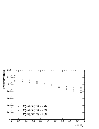
Figure 6: Angle between the electron and the neutrino in the $\Xi^{0}$ rest frame for different values of the ratio $F_{1}^{A}(0)/F_{1}^{V}(0)$.

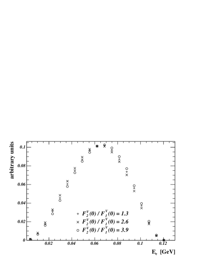
Figure 7: Energy spectrum of the electron for different values of the ratio $F_{2}^{V}(0)/F_{1}^{V}(0)$ in the $\Xi^{0}$ rest frame.

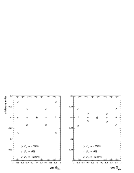
Figure 8: Left: Angle between $\Sigma^{+}$ and $x$ axis in the $\Xi^{0}$ rest frame. Right: Angle between proton and $x$ axis in the $\Sigma^{+}$ rest frame for different initial state polarizations of the $\Xi^{0}$ hyperon.

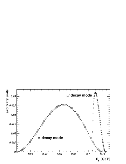
Figure 9: Comparison of lepton spectra for the e– and $\mu$–mode

The implementation was done as follows. We first generated the 3-body phase space of the primary decay $\Xi^{0}\to\Sigma^{+}+W^{-}_{\rm{off-shell}}$ using the widely used function genbod from the CERNLIB [72] library. Without loss of generality, the axis of the initial state polarization of the parent baryon was chosen to point along the lab $x$–axis. The momenta of the decay products of the secondary decays $\Sigma^{+}\to p+\pi^{0}$ and $W^{-}_{\rm{off-shell}}\to l^{-}+\bar{\nu}_{l}$ were generated with uniformly distributed directions. Since the secondary decays are two-body decays, the moduli of the respective momenta are fixed. The resulting momentum vectors were used to obtain the angles and momenta needed to calculate the value of the matrix element. This result was multiplied by the phase space factor of the primary decay returned by the genbod routine. Applying an acceptance-rejection method, the whole procedure was repeated until a generated event was no longer discarded.

In Fig. 6 we show a plot of the dependence of the rate on the angle between the electron and the neutrino in the $\Xi^{0}$ rest frame. In order to exhibit the sensitivity of this distribution to the form factor ratio $F_{1}^{A}(0)/F_{1}^{V}(0)$ we also show corresponding distributions with slightly varied form factor ratios. We mention that the distribution Fig. 6 and the following distributions are normalized to unity.

In Fig. 7 we show the electron energy spectrum and its dependence on the form factor ratio $F_{2}^{V}(0)/F_{1}^{V}(0)$. In Fig. 8 we show plots of the angular dependence of the angle between the $\Sigma^{+}$ and the $x$ axis in the $\Xi^{0}$ rest frame (left) and between the proton and the $x$ axis in the $\Sigma^{+}$ rest frame (right) for different polarizations of the parent $\Xi^{0}$ hyperon. In order to demonstrate the dependence on lepton mass effects, in Fig. 9 we show the energy spectra of the electron and the muon in the rest frame of the parent $\Xi^{0}$.

8 Summary and conclusions

We have worked out the angular decay distributions that govern the semileptonic cascade decay $\Xi^{0}\to\Sigma^{+}(\to p+\pi^{0})+W^{-}_{\rm{off-shell}}(\to l^{-}+\bar{\nu}_{l})$ using a cascade-type analysis. The cascade-type analysis has certain advantages, the main advantage being that one obtains the decay distributions in a compact quasi-factorized form. This leads to rather compact forms for the decay distributions. In our analysis we have included lepton mass effects as well as polarization effects of the decaying parent hyperon. We have always indicated the necessary sign changes when going from the $(l^{-},\bar{\nu}_{l})$ case to the $(l^{+},\nu_{l})$ case. Our angular decay formulae are thus applicable also to the semileptonic hyperon decay $\Sigma^{+}\to\Lambda+e^{+}+\nu_{e}$, or to semileptonic charm baryon decays induced by the transition $c\to s+l^{+}+\nu_{l}$ and also to the decays $t\to b+l^{+}+\nu_{l}$ . It should be clear that our angular decay formula are also applicable to the corresponding nonleptonic baryon decays involving vector mesons $(\lambda_{W}=\pm,0)$ or pseudoscalar mesons $(\lambda_{W}=t)$. In this case one has to omit the interference contributions between the time-component and the space-components of the currents.

Of interest are also the corresponding semileptonic antihyperon decays. The angular decay distributions of semileptonic antihyperon decays can be obtained from the corresponding angular decay distributions of the semileptonic hyperon decays by the replacements $H_{\lambda_{2}\lambda_{W}}(B)\to H_{\lambda_{2}\lambda_{W}}(\bar{B})$, $\alpha_{B}\to\alpha_{\bar{B}}$ and changing from the $(l^{-},\bar{\nu}_{l})$ to the $(l^{+},\nu_{l})$ case (or vice versa). Neglecting again $CP$–violating effects one has from $CP$-invariance $H_{\lambda_{2},\lambda_{W}}(\bar{B})=H_{-\lambda_{2},-\lambda_{W}}(B)$ and $\alpha_{\bar{B}}=-\alpha_{B}$. One can verify that the decay distributions in Eqs. (5.3.1), (66) and (6) are form invariant under $H_{\lambda_{2}\lambda_{W}}\to H_{-\lambda_{2}-\lambda_{W}}$, $\alpha_{B}\to-\alpha_{B}$ and $P\to-P$ as follows from $CP$–invariance. We mention that the NA48 collaboration has recently observed the decay $\overline{\Xi^{0}}\to\overline{\Sigma^{+}}e^{+}\nu_{e}$ and, based on 555 events, have given a branching ratio of $(2.55\pm 0.14_{{\rm stat}}\pm 0.10_{{\rm syst}})\cdot 10^{-4}$ for this semileptonic antihyperon decay [53].

We have summed over the helicity states of the final particles assuming that their polarization go unobserved. This corresponds to taking the trace of the density matrix of the final particles. It is clear that one can equally well calculate the density matrix of the final state particles by leaving the relevant helicity index unsummed. This was illustrated for the density matrix of the final lepton in the semileptonic decay process.

Doing the helicity sums in the master formulas listed in this paper by hand can become quite cumbersome. However, this task can be automated and can be left to the computer. The relevant Mathematica codes can be obtained from A. Kadeer. We mention also that the helicity frame analysis used in this paper can be easily transcribed to a transversality frame analysis (see e.g. [24]) where the $z$–axis is perpendicular to the hadron plane . In fact, any choice of $z$–axis in the analysis will provide the same total amount of information on the dynamics of the process entailed in the invariant amplitudes. It is then a question of experimental exigency of whether to analyze angular decay distributions in the helicity frame or the transversality frame, or, for that matter, in any other frame.

For the sake of conciseness we have written our results in terms of bilinear products of the helicity amplitudes $H_{\lambda_{2}\lambda_{W}}=H_{\lambda_{2}\lambda_{W}}^{V}+H_{\lambda_{2}\lambda_{W}}^{A}$ instead of bilinear products of the vector and axial vector helicity amplitudes $H_{\lambda_{2}\lambda_{W}}^{V}$ and $H_{\lambda_{2}\lambda_{W}}^{A}$. Writing the decay distributions in terms of $H_{\lambda_{2}\lambda_{W}}^{V}$ and $H_{\lambda_{2}\lambda_{W}}^{A}$ can be quite illuminating if one wishes to identify the overall parity nature of the observables that multiply the angular terms in the angular decay distributions.

We have formulated a minimal form factor model assuming $SU(3)$ symmetry at zero momentum transfer and a canonical $q^{2}$–dependence of the form factors. We have used this minimal form factor model to numerically calculate a few observables such as branching rates, the rate ratio $\Gamma(e)/\Gamma(\mu)$, a lepton–side forward-backward asymmetry, the longitudinal and transverse polarizations of the daughter baryon and the lepton and a mean azimuthal correlation parameter in the decay $\Xi^{0}\to\Sigma^{+}(\to p+\pi^{0})+l^{-}+\bar{\nu}_{l}$.

We have written a Monte Carlo event generator which is based on the angular decay distributions derived in this paper. Among others, the event generator allows one to generate events in the parent baryon rest frame. The MC program can be obtained from Rainer Wanke of the NA48 Collaboration (Rainer.Wanke@uni-mainz.de). We have presented a few decay distributions and correllations based on this event generator. We have, however, not systematically investigated which observables would be optimal to obtain the maximal possible information on the underlying dynamics encapsuled in the invariant form factors or the helicity amplitudes. A discussion of these issues also using parent baryon rest frame decays can be found in e.g. [7].

We did not provide an in–depth analysis of the dynamics of semileptonic hyperon decays as is necessary if one wants to extract a value of the CKM matrix element $V_{us}$ from semileptonic hyperon decay data. This issue was discussed in [56, 57, 58, 59]. We mention that there has been some recent progress in the dynamical description of strangeness changing semileptonic hyperon transition form factors from the lattice community [60, 61, 62] and in the framework of chiral symmetry [47, 66] including the explicit calculation of chiral corrections [63, 64, 65].

We finally emphasize that we have not included $CP$–violating effects or radiative corrections in our analysis. The latter can be included using the results of [7]. It will be interesting to find out how the radiative corrections will affect the angular decay distributions.

Acknowledgements: One of the authors (J. G. K.) acknowledges discussions, and e-mail and fax exchanges with I. Shipsey on whose insistence the sign mistake of the azimuthal correlation term in [28] was discovered and rectified. J. G. K. would also like to thank K. Zalewski for sharing his many insights into the subject of angular decay distributions in particle physics. U.M. would like to thank E.C. Swallow for valuable discussions. A. Kadeer acknowledges the support of the DFG (Germany) through the Graduiertenkolleg “Eichtheorien” at the University of Mainz.

Appendix A Two-body decay of a polarized particle in the helicity formalism

In deriving the two–body decay of a polarized spin $J$ particle in the helicity formalism we shall closely follow the approach of [67, 68]. Consider the two particle decay $a\to b+c$ of a spin $J_{a}$ particle where the polarization of particle $a$ in the frame $(x_{0},y_{0},z_{0})$ is given by $\rho^{0}_{\lambda_{a}\lambda^{\prime}_{a}}$. Consider a second frame $(x,y,z)$ obtained from $(x_{0},y_{0},z_{0})$ by the rotation $R(\theta,\phi,0)$ and whose $z$–axis is defined by particle $b$. The polarization density matrix $\rho$ in the frame $(x,y,z)$ is obtained by a “rotation” of the density matrix $\rho^{0}$ from the frame $(x_{0},y_{0},z_{0})$ to the frame $(x,y,z)$. The rate for $a\to b+c$ is then given by the the sum of the decay probabilities $|H_{\lambda_{b}\lambda_{c}}|^{2}$ (with $\lambda_{a}=\lambda_{b}-\lambda_{c}$) weighted by the diagonal terms of the density matrix $\rho$ of particle a in the frame $(x,y,z)$. Thus we find

$$\Gamma_{a\to b+c}(\theta,\phi)\propto\sum_{\lambda_{a},\lambda^{\prime}_{a},\lambda_{b},\lambda_{c}} |H_{\lambda_{b}\lambda_{c}}|^{2}D^{J*}_{\lambda_{a},\lambda_{b}-\lambda_{c}}(\theta,\phi)\,\rho^{0}_{\lambda_{a},\lambda^{\prime}_{a}}D^{J}_{\lambda^{\prime}_{a},\lambda_{b}-\lambda_{c}}(\theta,\phi)\,$$ (A1)

where

$$D^{J}_{m,m^{\prime}}(\theta,\phi)=e^{-im\phi}d^{J}_{m\,m^{\prime}}(\theta)\,\,.$$ (A2)

All the master formulas written down in this paper can be obtained by a repeated application of the basic two-body formula Eq. (A1).

Appendix B Wigner’s $d^{J}$–functions for J=1/2 and J=1

For definiteness we list explicit forms for the two $d^{J}$–functions of Wigner used in this paper. We use the convention of Rose [69] which is also the convention of [49] . One has

$$d^{1/2}_{mm^{\prime}}(\theta)=\left(\begin{array}[]{cc}\cos\theta/2&-\sin\theta/2\\ \sin\theta/2&\cos\theta/2\end{array}\right)$$ (B1)

for $J={\textstyle\frac{1}{2}}$ and

$$d^{1}_{mm^{\prime}}(\theta)=\left(\begin{array}[]{ccc}\frac{1}{2}(1+\cos\theta)&-\frac{1}{\sqrt{2}}\sin\theta&\frac{1}{2}(1-\cos\theta)\\ \frac{1}{\sqrt{2}}\sin\theta&\cos\theta&-\frac{1}{\sqrt{2}}\sin\theta\\ \frac{1}{2}(1-\cos\theta)&\frac{1}{\sqrt{2}}\sin\theta&\frac{1}{2}(1+\cos\theta)\end{array}\right)\vspace{0.5cm}$$ (B2)

for $J=1$. The rows and columns are labeled in the order $(1/2,-1/2)$ and $(1,0,-1)$, respectively.

Appendix C $T$–odd contributions

In the main text we have assumed that the invariant form factors and thereby the helicity amplitudes are relatively real. If one allows for relative phases between the helicity amplitudes one will obtain so–called $T$–odd contributions in the angular decay distributions. They appear in the azimuthal correlation terms as can be seen by the following example taken from the joint angular decay distribution in Sec. 6. One of the azimuthal correlation terms derives from the helicity configurations $(\lambda_{2}=-1/2,\lambda_{W}=0;\lambda^{\prime}_{2}=1/2,\lambda^{\prime}_{W}=1)$ and $(\lambda_{2}=1/2,\lambda_{W}=1;\lambda^{\prime}_{2}=-1/2,\lambda^{\prime}_{W}=0)$. Picking out the relevant terms in the master formula Eq. (6) one has

$$H_{\frac{1}{2}1}H^{*}_{-\frac{1}{2}0}\,e^{i(\pi-\chi)}+H_{-\frac{1}{2}0}H^{*}_{\frac{1}{2}1}\,e^{-i(\pi-\chi)}=-2\cos\!\chi\,\rm{Re}(H_{\frac{1}{2}1}H^{*}_{-\frac{1}{2}0})-2\sin\!\chi\,\rm{Im}(H_{\frac{1}{2}1}H^{*}_{-\frac{1}{2}0})\,\,.$$ (C1)

The $\cos\!\chi$ dependent term already appears in Eq. (6) whereas the $\sin\!\chi$ dependent term has been dropped in Eq. (6) because of the relative reality assumption for the helicity amplitudes. Adding the relevant $\theta$ and $\theta_{B}$ dependent trigonometric functions in the above azimuthal correlation term one has the two angle dependent $T$–odd terms ($\sin\theta\sin\!\chi\sin\theta_{B}\,\rm{Im}(H_{\frac{1}{2}1}H^{*}_{-\frac{1}{2}0}$)) and ($\cos\theta\sin\theta\sin\!\chi\sin\theta_{B}\,\rm{Im}(H_{\frac{1}{2}1}H^{*}_{-\frac{1}{2}0}$)) proportional to $\sin\!\chi$.

Next we rewrite the product of angular factors in terms of scalar and pseodoscalar products using the momentum representations in the $(x,y,z)$–system (see Fig. 5). For the normalized momenta one has $(\hat{p}^{2}=1)$

$$\hat{p}_{l^{-}} = (\sin\theta\cos\chi,\sin\theta\sin\chi,-\cos\theta)\,,$$ (C2)

$$\hat{p}_{W} = (0,0,-1)\,,$$

$$\hat{p}_{\Sigma^{+}} = (0,0,1)\,,$$

$$\hat{p}_{p} = (\sin\theta_{B},0,\cos\theta_{B})\,,$$

where the momenta have unit length indicated by a hat notation. The above T–odd angular factors can then be rewritten as

$$\sin\theta\sin\chi\sin\theta_{B} = \hat{p}_{W}\!\cdot\left(\hat{p}_{l^{-}}\!\times\hat{p}_{p}\right)\,,$$ (C3)

$$\cos\theta\sin\theta\sin\chi\sin\theta_{B} = (\hat{p}_{l^{-}}\cdot\hat{p}_{W})\,[\,\hat{p}_{W}\cdot\left(\,\hat{p}_{l^{-}}\!\times\hat{p}_{p}\right)]\,.$$

Under time reversal ($t\to-t$) one has $(p\to-p)$. Since the $T$–odd momenta invariants in Eq. (C3) involve an odd number of momenta they change sign under time reversal. This has led to the notion of the so–called $T$–odd obsevables. Observables that multiply $T$–odd momentum invariants are called $T$–odd obsevables. They can be contributed to by true $CP$–violating effects or by final state interaction effects unless either or both change all helicity amplitudes by the same common phase. One may distinguish between the two sources of $T$–odd effects by comparing with the corresponding antihyperon decays since phases from $CP$–violating effects change sign whereas phases from final state interaction effects do not change sign when going from hyperon to antihyperon decays.

From the above example it should be clear how to obtain the $T$–odd contributions from the master formulas for the other cases. In practise what one has to do is to add terms where the real part of the bilinear forms of helicity amplitudes is replaced by the corresponding imaginary part and the cosine of the azimuthal angle is replaced by the sine with a possible sign change.

Appendix D Full five-fold angular decay distribution

In this appendix we write down the full five-fold angular decay distribution for the semileptonic cascade decay of a polarized hyperon. There are now altogether three polar angles $\theta$, $\theta_{B}$ and $\theta_{P}$, where $\theta_{P}$ describes the polar orientation of the polarization vector of the parent hyperon as shown in Fig. 10 (which is directly taken from [18]). Since there are now two planes in the cascade decay, there is one more azimuthal angle which we choose as $\phi_{l}$ as shown in Fig. 11. It is important to note that Fig. 11 shows a special configuration where the momentum of the proton lies in the first quadrant and the momentum of the lepton lies in the second quadrant. It is clear that, for this special configuration, the three azimuthal angles $\phi_{l},\phi_{B}$ and $\chi$ add up to $\pi$ ($\phi_{l}+\phi_{B}+\chi=\pi$). For other configurations it may happen that the three angles add up to $\pi+\rm{mod}(2\pi)$ if the rotation sense of the angles in Fig. 11 is kept. This will be of no consequence for the angular decay distribution which is invariant under azimuthal $2\pi$ shifts.

The full five-fold angular decay distribution can be directly taken from [18] after including the appropriate sign changes going from the $(l^{+},\nu_{l})$ to the $(l^{-},\bar{\nu}_{l})$ case. We have simplified the corresponding expressions in [18] by assuming as before that the helicity amplitudes are real. For completeness we shall also write down the decay distribution in explicit form using Wigner’s $d^{J}$–functions as before. One has the master formula

$$W(\theta,\theta_{P},\theta_{B},\phi_{B},\phi_{l})\propto \sum_{\lambda_{l},\lambda_{W},\lambda^{\prime}_{W},J,J^{\prime},\lambda_{2},\lambda_{2}^{\prime},\lambda_{3}}(-1)^{J+J^{\prime}}|h^{l}_{\lambda_{l}\lambda_{\nu=\pm 1/2}}|^{2}e^{i(\lambda_{W}-\lambda^{\prime}_{W})\phi_{l}}\times$$

$$\times\rho_{\lambda_{2}-\lambda_{W},\lambda^{\prime}_{2}-\lambda^{\prime}_{W}}(\theta_{P})d^{J}_{\lambda_{W},\lambda_{l}-\lambda_{\nu}}(\theta)d^{J^{\prime}}_{\lambda^{\prime}_{W},\lambda_{l}-\lambda_{\nu}}(\theta)H_{\lambda_{2}\lambda_{W}}H^{*}_{\lambda^{\prime}_{2}\lambda^{\prime}_{W}}\times$$

$$\times e^{i(\lambda_{2}-\lambda^{\prime}_{2})\phi_{B}}d^{\frac{1}{2}}_{\lambda_{2}\lambda_{3}}(\theta_{B})d^{\frac{1}{2}}_{\lambda_{2}^{\prime}\lambda_{3}}(\theta_{B})|h^{B}_{\lambda_{3}0}|^{2}\,.$$ (D1)

Figure 10: Definition of the three polar angles $\theta$, $\theta_{B}$ and $\theta_{P}$ in the semileptonic decay of a polarized $\Xi^{0}$ into $\Sigma^{+}+l^{-}+\bar{\nu}_{l}$ followed by the nonleptonic decay $\Sigma^{+}\to p+\pi^{0}$. The polarization vector of the parent baryon $\vec{P}$ lies in the $(x,z)$–plane with positive $P_{x}$ component.

Figure 11: Definition of the three azimuthal angles $\phi_{l}$, $\phi_{B}$ and $\chi$ ($\phi_{l}+\phi_{B}+\chi=\pi$) in the semileptonic decay of a polarized $\Xi^{0}$. Fig. 11 is a view of Fig. 10 from the right along the negative $z$–direction. $\vec{p}_{l}^{T}$ and $\vec{p}_{p}^{T}$ denote the transverse components of the momentum of the lepton and proton, respectively.

For the normalized five-fold angular decay distribution one finds

$$\frac{d\Gamma}{dq^{2}d\cos\theta_{B}d\cos\theta d\cos\theta_{P}d\chi d\phi_{l}} =B(B_{2}\to B_{3}+M)\frac{1}{12}\frac{G_{F}^{2}}{(2\pi)^{5}}|V_{us}|^{2}\frac{(q^{2}-m_{l}^{2})^{2}p}{8M_{1}^{2}q^{2}}\times$$

$$\times\bigg{[}b_{00}^{00}+3\cos\theta\ b_{00}^{01}+\cos{\theta_{B}}\ b_{00}^{10}$$

$$+(\frac{3}{2}\cos^{2}{\theta}-\frac{1}{2})\ b_{00}^{02}$$

$$-3\sqrt{2}\sin{\theta}\cos{\phi_{l}}\ b_{01}^{01}$$

$$-2\sin{\theta_{B}}\cos{\phi_{B}}\ b_{10}^{10}$$

$$-\frac{3}{\sqrt{2}}\sin{2\theta}\cos{\phi_{l}}\ b_{01}^{02}$$

$$+3\cos{\theta}\cos{\theta_{B}}\ b_{00}^{11}$$

$$+(\frac{3}{2}\cos^{2}{\theta}-\frac{1}{2})\cos{\theta_{B}}\ b_{00}^{12}$$

$$-\frac{3}{2}\sqrt{2}\sin{\theta}\sin{\theta_{B}}\cos{\chi}\ b_{11}^{11}$$

$$-\frac{3}{4}\sqrt{2}\sin{\theta_{B}}\sin{2\theta}\cos{\chi}\ b_{11}^{12}$$

$$+\frac{3}{2}\sin^{2}\theta\sin{\theta_{B}}\cos(\chi-\phi_{l})\ b_{12}^{12}$$

$$-6\cos{\theta}\sin{\theta_{B}}\ \cos\phi_{B}\ b_{10}^{11}$$

$$-3\sqrt{2}\sin{\theta}\cos{\theta_{B}}\cos{\phi_{l}}\ b_{01}^{11}$$

$$-\frac{3}{2}\sqrt{2}\sin{2\theta}\cos{\theta_{B}}\cos{\phi_{l}}\ b_{01}^{12}$$

$$-\sin{\theta_{B}}(3\cos^{2}{\theta}-1)\cos\phi_{B}b_{10}^{12}\,\,\,\bigg{]}\,.$$ (D2)

It is important that the rotation sense of the azimuthal angles in Fig. 11 is kept. We have used the relation $\phi_{l}+\phi_{B}+\chi=\pi+\rm{mod}(2\pi)$ to rewrite $\cos(\phi_{B}+\phi_{l})=-\cos\chi$ and $\cos(\phi_{B}+2\phi_{l})=-\cos(\chi-\phi_{l})$. Note that Eq. (D) contains the redundant angle $\phi_{B}$. As before one can reexpress $\cos\phi_{B}$ as $\cos\phi_{B}=-\cos(\phi_{l}+\chi)$.

The coefficients $b^{kl}_{ij}$ in Eq. (D) are given by

$$b_{00}^{00}= \Big{(}(1+\epsilon)(|H_{-\frac{1}{2}-1}|^{2}+|H_{\frac{1}{2}0}|^{2})+3\epsilon|H_{\frac{1}{2}t}|^{2}\Big{)}\,\rho_{\frac{1}{2}\frac{1}{2}}$$

$$+\Big{(}(1+\epsilon)(|H_{\frac{1}{2}1}|^{2}+|H_{-\frac{1}{2}0}|^{2})+3\epsilon|H_{-\frac{1}{2}t}|^{2}\Big{)}\rho_{-\frac{1}{2}-\frac{1}{2}},$$

$$b_{00}^{01}= \frac{1}{2}\Big{(}\mp|H_{\frac{1}{2}1}|^{2}-4\epsilon\ H_{-\frac{1}{2}0}H_{-\frac{1}{2}t}\Big{)}\,\rho_{-\frac{1}{2}-\frac{1}{2}}$$

$$-\frac{1}{2}\Big{(}\mp|H_{-\frac{1}{2}-1}|^{2}+4\epsilon\ H_{\frac{1}{2}0}H_{\frac{1}{2}t}\Big{)}\,\rho_{\frac{1}{2}\frac{1}{2}}\,,$$

$$b_{00}^{10}= \alpha_{B}\Big{(}(1+\epsilon)(-|H_{-\frac{1}{2}-1}|^{2}+|H_{\frac{1}{2}0}|^{2})+3\epsilon|H_{\frac{1}{2}t}|^{2}\Big{)}\rho_{\frac{1}{2}\frac{1}{2}}$$

$$-\alpha_{B}\Big{(}(1+\epsilon)(|H_{-\frac{1}{2}0}|^{2}\!-\!|H_{\frac{1}{2}1}|^{2})\!+\!3\epsilon|H_{-\frac{1}{2}t}|^{2}\Big{)}\rho_{-\frac{1}{2}-\frac{1}{2}},$$

$$b_{00}^{02}= \frac{1-2\epsilon}{2}\Big{(}-2|H_{-\frac{1}{2}0}|^{2}+|H_{\frac{1}{2}1}|^{2}\Big{)}\,\rho_{-\frac{1}{2}-\frac{1}{2}}$$

$$+\frac{1-2\epsilon}{2}\Big{(}|H_{-\frac{1}{2}-1}|^{2}-2|H_{\frac{1}{2}0}|^{2}\Big{)}\,\rho_{\frac{1}{2}\frac{1}{2}}\,,$$

$$b_{01}^{01}= \frac{1}{2}\Big{(}2\epsilon H_{-\frac{1}{2}t}H_{-\frac{1}{2}-1}\pm H_{-\frac{1}{2}0}H_{-\frac{1}{2}-1}$$

$$-2\epsilon H_{\frac{1}{2}1}H_{\frac{1}{2}t}\pm H_{\frac{1}{2}1}H_{\frac{1}{2}0}\Big{)}\,\rho_{\frac{1}{2}-\frac{1}{2}}\,,$$

$$b_{10}^{10}= -\alpha_{B}\Big{(}3\epsilon H_{\frac{1}{2}t}H_{-\frac{1}{2}t}+(1+\epsilon)H_{\frac{1}{2}0}H_{-\frac{1}{2}0}\Big{)}\,\rho_{-\frac{1}{2}\frac{1}{2}}\,,$$

$$b_{01}^{02}= \frac{1-2\epsilon}{2}\Big{(}H_{-\frac{1}{2}0}H_{-\frac{1}{2}-1}-H_{\frac{1}{2}1}H_{\frac{1}{2}0}\Big{)}\,\rho_{\frac{1}{2}-\frac{1}{2}}\,,$$

$$b_{00}^{11}= \frac{\alpha_{B}}{2}\Big{(}\mp|H_{\frac{1}{2}1}|^{2}+4\epsilon\ H_{-\frac{1}{2}0}H_{-\frac{1}{2}t}\Big{)}\,\rho_{-\frac{1}{2}-\frac{1}{2}}$$

$$+\frac{\alpha_{B}}{2}\Big{(}\mp|H_{-\frac{1}{2}-1}|^{2}-4\epsilon\ H_{\frac{1}{2}0}H_{\frac{1}{2}t}\Big{)}\,\rho_{\frac{1}{2}\frac{1}{2}}\,,$$

$$b_{00}^{12}= \frac{\alpha_{B}}{2}(1-2\epsilon)\Big{(}2|H_{-\frac{1}{2}0}|^{2}+|H_{\frac{1}{2}1}|^{2}\Big{)}\,\rho_{-\frac{1}{2}-\frac{1}{2}}$$

$$-\frac{\alpha_{B}}{2}(1-2\epsilon)\Big{(}|H_{-\frac{1}{2}-1}|^{2}+2|H_{\frac{1}{2}0}|^{2}\Big{)}\,\rho_{\frac{1}{2}\frac{1}{2}}\,,$$

$$b_{11}^{11}= \alpha_{B}\Big{(}2\epsilon H_{\frac{1}{2}1}H_{-\frac{1}{2}t}\mp H_{\frac{1}{2}1}H_{-\frac{1}{2}0}\Big{)}\,\rho_{-\frac{1}{2}-\frac{1}{2}}$$

$$+\alpha_{B}\Big{(}-2\epsilon H_{\frac{1}{2}t}H_{-\frac{1}{2}-1}\mp H_{\frac{1}{2}0}H_{-\frac{1}{2}-1}\Big{)}\,\rho_{\frac{1}{2}\frac{1}{2}}\,,$$

$$b_{11}^{12}= \alpha_{B}(1-2\epsilon)\Big{(}H_{\frac{1}{2}1}H_{-\frac{1}{2}0}\,\rho_{-\frac{1}{2}-\frac{1}{2}}-H_{\frac{1}{2}0}H_{-\frac{1}{2}-1}\,\rho_{\frac{1}{2}\frac{1}{2}}\Big{)}\,,$$

$$b_{12}^{12}= -\alpha_{B}(1-2\epsilon)H_{\frac{1}{2}1}H_{-\frac{1}{2}-1}\,\rho_{\frac{1}{2}-\frac{1}{2}}\,,$$

$$b_{10}^{11}= \alpha_{B}\,\epsilon\,\Big{(}H_{\frac{1}{2}0}H_{-\frac{1}{2}t}+H_{\frac{1}{2}t}H_{-\frac{1}{2}0}\Big{)}\,\rho_{-\frac{1}{2}\frac{1}{2}}\,,$$

$$b_{01}^{11}= \frac{\alpha_{B}}{2}\Big{(}-2\epsilon H_{-\frac{1}{2}t}H_{-\frac{1}{2}-1}\mp H_{-\frac{1}{2}0}H_{-\frac{1}{2}-1}$$

$$-2\epsilon H_{\frac{1}{2}1}H_{\frac{1}{2}t}\pm H_{\frac{1}{2}1}H_{\frac{1}{2}0}\Big{)}\,\rho_{\frac{1}{2}-\frac{1}{2}}\,,$$

$$b_{01}^{12}= -\frac{\alpha_{B}}{2}(1-2\epsilon)\Big{(}H_{-\frac{1}{2}0}H_{-\frac{1}{2}-1}+H_{\frac{1}{2}1}H_{\frac{1}{2}0}\Big{)}\,\rho_{\frac{1}{2}-\frac{1}{2}}\,,$$

$$b_{10}^{12}= \alpha_{B}(1-2\epsilon)H_{\frac{1}{2}0}H_{-\frac{1}{2}0}\,\rho_{-\frac{1}{2}\frac{1}{2}}\,.$$ (D3)

We have introduced the abbreviation $\epsilon=m_{l}^{2}/2q^{2}$ for the leptonic flip suppression factor. As in the main text the upper signs in the coefficients $b^{kl}_{ij}$ hold for the case $(l^{-},\bar{\nu}_{l})$ relevant to the cascade decay $\Xi^{0}\to\Sigma^{+}(\to p+\pi^{0})+l^{-}+\bar{\nu}_{l}$ treated in this paper. The lower signs hold for the case $(l^{+},\nu_{l})$ discussed in [18]. Finally, $\rho_{\lambda_{1}\lambda_{1}^{{}^{\prime}}}$ is the spin density matrix of the parent hyperon given in Eq. (61).

We have performed various checks on Eq. (D). First we found it to agree with the angular decay distribution derived from the master formula Eq. (D). We further checked that Eq. (D) reduces to the decay distributions listed in the main text after integration or after setting the relevant parameters to zero. We thus checked that Eq. (D) reduces to Eq. (6) when setting $P=0$. There is a factor of $4\pi$ from the integration over $\cos\theta_{P}$ and $\phi_{l}$. Further Eq. (D) reduces to Eq. (5.3.1) when setting $\alpha_{B}=0$, dropping the branching ratio factor $B(B_{2}\to B_{3}+M)$ and replacing $\phi_{l}$ by $(\pi-\chi)$. Also there is a factor $4\pi$ from the integration over $\cos\theta_{B}$ and $\phi_{B}$. Finally, Eq. (D) reduces to Eq. (66) when integrating over $\phi_{l}$ and $\cos\theta$. As mentioned before we have assumed that the helicity amplitudes (or the invariant amplitudes) are relatively real. Nonzero relative phases between the helicity amplitudes could arise from final state interaction effects or from extensions of the SM that bring in $CP$–violating phases (see e.g. [70, 71]). In such a case one would have to keep the full phase structure contained in the master formula Eq. (D) or in the original version of Eq. (D) listed in [18].

References

• [1] C.H. Albright, Phys. Rev. 115 (1959) 750.
• [2] D.R. Harrington, Phys. Rev. 120 (1960) 1482.
• [3] M.M. Nieto, Rev. Mod. Phys. 40 (1968) 140.
• [4] I. Bender, V. Linke and H. J. Rothe, Z. Phys. 212 (1968) 190.
• [5] V. Linke, Nucl. Phys. B 12 (1969) 669.
• [6] V. Linke, Nucl. Phys. B 23 (1970) 376.
• [7] A. Garcia and P. Kielanowski, The Beta Decay of Hyperons, Lecture Notes in Physics Vol. 222 (Springer-Verlag, Berlin, 1985).
• [8] W. Alles, Nuovo Cimento 26 (1962) 1429.
• [9] J. M. Watson and R. Winston, Phys. Rev.  181 (1969) 1907.
• [10] S. Bright, R. Winston, E. C. Swallow and A. Alavi-Harati, Phys. Rev. D 60 (1999) 117505 [Erratum-ibid. D 62 (2000) 059904].
• [11] A. Kotański and K. Zalewski, Nucl. Phys. B 4 (1968) 559.
• [12] A. Kotański, B. Sredniawa and K. Zalewski, Nucl. Phys. B 23 (1970) 541.
• [13] A. Kotański and K. Zalewski, Nucl. Phys. B 22 (1970) 317.
• [14] J. Dabkowski, Nucl. Phys. B 33 (1971) 621.
• [15] J. G. Körner and G. R. Goldstein, Phys. Lett. B 89 (1979) 105.
• [16] G. Kramer and W. F. Palmer, Phys. Rev. D 45 (1992) 193.
• [17] J. G. Körner and H. W. Siebert, Ann. Rev. Nucl. Part. Sci.  41 (1991) 511.
• [18] P. Bialas, J. G. Körner, M. Krämer and K. Zalewski, Z. Phys. C 57 (1993) 115.
• [19] J. G. Körner, M. Krämer and D. Pirjol, Prog. Part. Nucl. Phys.  33 (1994) 787, arXiv: hep-ph/9406359.
• [20] S. Shulga, arXiv: hep-ph/0501207.
• [21] Z. J. Ajaltouni, E. Conte and O. Leitner, Phys. Lett. B 614 (2005) 165.
• [22] O. Leitner, Z. J. Ajaltouni and E. Conte, Nucl. Phys. A 755 (2005) 435.
• [23] J. G. Körner and G. A. Schuler, Z. Phys. C 38 (1988) 511 [Erratum-ibid. C 41 (1989) 690].
• [24] J. G. Körner and G. A. Schuler, Z. Phys. C 46 (1990) 93.
• [25] K. Hagiwara, A. D. Martin and M. F. Wade, Phys. Lett. B 228 (1989) 144.
• [26] K. Hagiwara, A. D. Martin and M. F. Wade, Nucl. Phys. B 327 (1989) 569.
• [27] K. Hagiwara, A.D. Martin and M.F. Wade, Z. Phys. C 46 (1990) 299.
• [28] J. G. Körner and M. Krämer, Phys. Lett. B 275 (1992) 495.
• [29] P. Bialas, K. Zalewski and J. G. Körner, Z. Phys. C 59 (1993) 117.
• [30] A. Ali and A. S. Safir, Eur. Phys. J. C 25 (2002) 583, arXiv: hep-ph/0205254.
• [31] A. Faessler, T. Gutsche, M. A. Ivanov, J. G. Körner and V. E. Lyubovitskij, Eur. Phys. J. directC 4 (2002) 18.
• [32] T. M. Aliev and M. Savci, arXiv: hep-ph/0507324.
• [33] P.H. Frampton and W.K. Tung, Phys. Rev. D3 (1971) 1114.
• [34] M. Fischer, S. Groote, J. G. Körner, M. C. Mauser and B. Lampe, Phys. Lett. B 451 (1999) 406.
• [35] M. Fischer, S. Groote, J. G. Körner and M. C. Mauser, Phys. Rev. D 63 (2001) 031501.
• [36] M. Fischer, S. Groote, J. G. Körner and M. C. Mauser, Phys. Rev. D 65 (2002) 054036.
• [37] H. S. Do, S. Groote, J. G. Körner and M. C. Mauser, Phys. Rev. D 67 (2003) 091501.
• [38] P.R. Auvil and J.J. Brehm, Phys. Rev. 145 (1966) 1152.
• [39] R. E. Behrends and A. Sirlin, Phys. Rev. Lett.  4 (1960) 186.
• [40] M. Ademollo and R. Gatto, Phys. Rev. Lett.  13 (1964) 264.
• [41] N. Brene et al., Phys. Lett. 11 (1964) 344.
• [42] S. Balk, J. G. Körner and D. Pirjol, Eur. Phys. J. C1 (1998) 221.
• [43] E. Byckling and K. Kajantie, Particle Kinematics, (John Wiley and Sons, 1973).
• [44] F. Hussain and J. G. Körner, Z. Phys. C 51 (1991) 607.
• [45] F. Hussain, J. G. Körner and R. Migneron, Phys. Lett. B 248 (1990) 406 [Erratum-ibid. B 252 (1990) 723].
• [46] J. G. Körner and M. Kuroda, Phys. Rev. D 16 (1977) 2165.
• [47] A. Faessler, T. Gutsche, B. R. Holstein, M. A. Ivanov, J. G. Körner and V. E. Lyubovitskij, arXiv: 0809.4159 [hep-ph].
• [48] J.L. Cortes, X.Y. Pham and A. Tonsi, Phys. Rev. D25 (1982) 188.
• [49] Particle Data Group, C. Amsler et al, Phys. Lett. B667 (2008) 1.
• [50] C. Lazzeroni [NA48 Collaboration], PoS HEP2005 (2006) 096.
• [51] R. Wanke, In the Proceedings of International Conference on Heavy Quarks and Leptons (HQL 06), Munich, Germany, 16-20 Oct 2006, pp 006, arXiv: hep-ex/0702019.
• [52] The KTeV Collaboration, E. Abouzaid et al, Phys. Rev. Lett.  95 (2005) 081801, arXiv: hep-ex/0504055.
• [53] J. R. Batley et al. [NA48/I Collaboration], Phys. Lett.  B 645 (2007) 36, arXiv: hep-ex/0612043.
• [54] H. Pietschmann, Weak Interactions -  Formulae, Results and Derivations, (Springer Verlag, 1983).
• [55] J. W. Hinson et al. [CLEO Collaboration], Phys. Rev. Lett.  94 (2005) 191801.
• [56] R. Flores-Mendieta, E. Jenkins and A. V. Manohar, Phys. Rev. D 58 (1998) 094028.
• [57] N. Cabibbo, E. C. Swallow and R. Winston, Phys. Rev. Lett.  92 (2004) 251803.
• [58] N. Cabibbo, E. C. Swallow and R. Winston, Ann. Rev. Nucl. Part. Sci.  53 (2003) 39.
• [59] V. Mateu and A. Pich, arXiv: hep-ph/0509045.
• [60] D. Guadagnoli, V. Lubicz, M. Papinutto and S. Simula, Nucl. Phys.  B 761 (2007) 63, arXiv: hep-ph/0606181.
• [61] S. Sasaki and T. Yamazaki, PoS LAT2006 (2006) 092, arXiv: hep-lat/0610082.
• [62] H. W. Lin, arXiv: 0707.3647 [hep-ph].
• [63] G. Villadoro, Phys. Rev.  D 74 (2006) 014018, arXiv: hep-ph/0603226.
• [64] A. Lacour, B. Kubis and U. G. Meissner, JHEP 0710 (2007) 083, arXiv: 0708.3957 [hep-ph].
• [65] F. J. Jiang and B. C. Tiburzi, Phys. Rev.  D 77 (2008) 094506, arXiv: 0801.2535 [hep-lat].
• [66] T. Ledwig, A. Silva, H. C. Kim and K. Goeke, arXiv: 0806.4072 [hep-ph].
• [67] J. D. Jackson, in “High Energy Physics”, 1965 Les Houches lectures, p. 325, (Gordon and Breach, New York, 1966).
• [68] W. K. Tung, Group Theory in Physics, (World Scientific, Philadelphia, Singapore, 1985).
• [69] M. E. Rose, Elementary Theory of Angular Momentum, (Wiley, New York, 1957).
• [70] J. G. Körner, K. Schilcher and Y. L. Wu, Phys. Lett. B 242 (1990) 119.
• [71] J. G. Körner, K. Schilcher and Y. L. Wu, Z. Phys. C 55 (1992) 479.
• [72] The function genbod can be obtained from http://cernlib.web.cern.ch/cernlib/.