Big Bang Nucleosynthesis Constraints on Universal Extra Dimensions and Varying Fundamental Constants

Abstract

The successful prediction of light element abundances from Big Bang Nucleosynthesis (BBN) has been a pillar of the standard model of Cosmology. Because many of the relevant reaction rates are sensitive to the values of fundamental constants, such as the fine structure constant and the strong coupling constant, BBN is a useful tool to probe and to put constraints on possible cosmological variations of these constants, which arise naturally from many versions of extra-dimensional theories. In this paper, we study the dependences of fundamental constants on the radion field of the universal extra dimension model, and calculate the effects of such varying constants on BBN. We also discussed the possibility that the discrepancy between BBN and the Wilkinson Microwave Anisotropy Probe (WMAP) data on the baryon-to-photon ratio can be reduced if the volume of the extra dimensions was slightly larger - by $\mathcal{O}(10^{-3})$ - at the BBN era compared to its present value, which would result in smaller gauge couplings at BBN by the same factor.

I INTRODUCTION

The standard Big Bang Nucleosynthesis (BBN) theory is a successful marriage between standard Friedmann cosmology and nuclear physics, explaining the origin and abundances of the light elements D, ⁴He, ³He and ⁷Li. Its only one input parameter, the baryon-to-photon ratio $\eta=n_{b}/n_{\gamma}$ (where $n_{b}$ and $n_{\gamma}$ are respectively the number density of baryons and photons) has now been determined by the observations of the Wilkinson Microwave Anisotropy Probe (WMAP) with rather good accuracy Spergel (2003), so that there are essentially no free parameters in this scenario. Because the BBN predictions are sensitive to a set of physical quantities which depend on various fundamental constants such as the gauge couplings, the Yukawa couplings and gravitational constant (see Sections III and IV for details), it would provide stringent constraints on the cosmological variations of these constants. For example, in Bergstrom (1999); Avelino (2001); Nollett (2002) the authors use BBN to constrain the change of fine structure constant, in Dixit (1988); Scherrer (1993); Yoo (2003) constraints on the change of Higgs vacuum expectation value are considered, and the effects of a varying strong coupling are discussed in e.g. Flambaum (2002); Kneller (2003); the variation of gravitational constant has also been investigated Casas (1992); Serna (1992); Santiago (1997); Damour (1999); Clifton (2005) in the context of BBN. Besides, there is another reason for the interests in the interplay between varying fundamental constants and BBN: in contrast to the excellent consistency between BBN theory and observation with $\eta$ given by WMAP for the deuteron (D) abundance, the predicted ⁴He and ⁷Li abundances are smaller than the results implied by WMAP Cyburt (2003); Steigman (2003); it is then suggested that the variations of fundamental constants such as the fine structure constant Nollett (2002); Ichikawa (2004) or the deuteron binding energy $B_{d}$ Dmitriev (2004) ($B_{d}$ itself is certainly not a fundamental constant, but its variation possibly originates from some other fundamental constants as suggested in Yoo (2003)) etc. might partly or completely solve this discrepancy.

The theoretical investigations of varying fundamental constants date back to the early work of Dirac in 1930’s, and have re-aroused great attentions because of the recent discovery of Webb et al. Webb (1999); Murphy (2001) that the quasar absorption lines at redshifts of $z$ = 1 $\sim$ 3 suggest a small evolution of the fine structure constant between that period and present. Although variations of the fundamental constants do not occur in the standard model (SM) of particle physics, the two leading paradigms of the physics beyond SM, namely the string theory Polchinski (1998) and the Kaluza Klein theory Overduin (1997), generally predict such variations. In these scenarios a dilaton field or the size of extra dimensions may evolve cosmologically; thus until their vacuum expectation values (VEV) are fixed, there might be a co-variation of several fundamental constants. This picture is similar to the discussions in grand unified theories (GUTs) Langacker (2002); Calmet (2002) and implies that considerations of one varying constant alone may be incomplete, although indeed such a co-variation itself is in general rather model-dependent (see Campbell (1995); Ichikawa (2002) for one case derived from string theory). For a detailed discussion of the theoretical and observational (experimental) aspects of varying fundamental constants, see Uzan (2003).

The recent interests in the extra dimensional theories have stimulated other considerations of varying fundamental constants. Of the frequently discussed extra dimension models, the original ADD ADD (1999) and RS RS (1999) brane models do not induce changes in the gauge couplings even though their moduli fields evolve Brax (2003, 2003) because of the conformal invariance of the gauge kinetic terms (see however Palma (2003) for an alternative), and so in this work we will concentrate on the universal extra dimension (UED) model, in which the fields can propagate in all dimensions. This model was first proposed in Appelquist (2001) and became extremely interesting for cosmology since it was found later that it predicted the presence of a stable massive particle, the lightest KK partner (LKP), which is a natural dark matter candidate (see Servant (2002); Kong (2005) and references therein for details). Our purpose in this work is twofold: firstly, we study how the fundamental constants in the low energy effective theory change if the size of the universal extra dimensions, the radion field, undergoes a slow cosmological evolution and to what extent the changes are allowed by the BBN observations; secondly, we show that if the volume of the extra space at the time of BBN is slightly larger than its present value, the discrepancy between BBN and WMAP discussed above may be reduced.

The arrangement of this work is the following: in Section II we derive the effective low energy actions for the gravitational and matter sectors in the model; then we shall find the radion dependences of the fundamental constants in Section III. In Section IV we briefly review the standard BBN, point out the most relevant physical quantities for its prediction and relate these quantities to the radion field. Section V contains the numerical results of this work, which are obtained by modifying the standard code of BBN Kawano (1992) and including the effects discussed in Section IV. Finally Section VI is devoted to discussion and conclusion. Throughout this work we assume 3 species of massless neutrinos as in the standard BBN and adopt the units $\hbar=c=1$.

II THE LOW ENERGY 4-DIMENSIONAL EFFECTIVE ACTIONS

Let us consider a general $4+n$ dimensional model, with $n$ being the number of the (universal) extra dimensions (although there may also be large extra dimensions, we do not consider them in this work). The full line element is given as:

$$ds^{2}=G_{AB}dX^{A}dX^{B}=g_{\mu\nu}dx^{\mu}dx^{\nu}+h_{ab}dy^{a}dy^{b},$$ (1)

where $\mu$, $\nu$ = 0, 1, 2, 3 label the four ordinary dimensions, $a$, $b$ = $4,\cdot\cdot\cdot,3+n$ denote extra dimensions and $A,B=0,1,2,\cdot\cdot\cdot,3+n$ the whole spacetime. For simplicity we shall not consider cross terms such as $G_{a\mu}$ in Eq. (1). The extra dimensions are assumed to compactify on an orbifold, and their coordinates $y_{a}$ take values in the range [0, 1]. The quantities $h_{ab}$ have dimensions of [Length]² since $y_{a}$ are dimensionless in our choice.

Because the energy range we are interested in is much lower than the inverse size of the universal extra dimensions, which is thought to be larger than several hundred GeV’s, it is adequate to consider only the zero modes of the metric. Then the effective 4-dimensional action (in the gravitational sector) can be obtained by dimensionally reducing Eq. (1) as:

$$S_{\mathrm{Gravity}} = \frac{1}{\kappa_{4+n}^{2}}\int d^{4+n}X\sqrt{|G|}R_{4+n}[G]$$ (2)

$$= \frac{1}{\kappa_{4}^{2}}\int d^{4}xd^{n}y\sqrt{|g|}\frac{\sqrt{|h|}}{V_{0}}\left[R_{4}\left[g\right]-\frac{1}{4}\partial_{\mu}h^{ab}\partial^{\mu}h_{ab}-\frac{1}{4}h^{ab}\partial_{\mu}h_{ab}\cdot h^{cd}\partial^{\mu}h_{cd}\right],$$

in which $|g|$, $|h|$ and $|G|$ are respectively the determinants of the metrics of the ordinary dimensions, the extra dimensions and the whole spacetime. $R_{4}[g]$ and $R_{4+n}[G]$ are the Ricci scalars of the ordinary 4 and the total $4+n$ dimensional spacetimes. $\kappa_{4},\kappa_{4+n}$ are related to the 4 and $4+n$ dimensional Planck masses via $\kappa_{4}^{2}=2M_{4}^{2}$ and $\kappa_{4+n}^{2}=2M_{4+n}^{2+n}$, while they themselves are connected by a volume suppression $\kappa_{4+n}^{2}=\kappa_{4}^{2}\cdot V$, with $V$ being a measure of the extra space volume whose present-day value is denoted by $V_{0}$ in Eq. (2) (Note that because of the specified choice of $V_{0}$ and because the higher dimensional quantity $\kappa_{4+n}$ is treated as a constant, the $\kappa_{4}$ above also takes its currently measured value and is a constant rather than a variable).

The effective 4-dimensional curvature term is not canonical in Eq. (2); to make it so, let us take the conformal transformation

$$g_{\mu\nu}\rightarrow e^{2\phi}g_{\mu\nu}$$ (3)

and choose the field $\phi$ to satisfy

$$\frac{\sqrt{|h|}}{V_{0}}e^{2\phi}=1.$$ (4)

Then we obtain the effective 4-dimensional gravitational action in the Einstein frame:

$$S_{\mathrm{Gravity}}=\frac{1}{\kappa_{4}^{2}}\int d^{4}x\sqrt{|g|}\left[R_{4}-\frac{1}{4}\partial_{\mu}h^{ab}\partial^{\mu}h_{ab}+\frac{1}{8}h^{ab}\partial_{\mu}h_{ab}\cdot h^{cd}\partial^{\mu}h_{cd}\right].$$ (5)

We shall make a further assumption that the extra dimension(s) are homogeneous and isotropic, i.e. the metric of the extra space takes the following form:

$$h_{ab}=\mathrm{diag}(-b^{2},-b^{2},\cdot\cdot\cdot,-b^{2}),$$ (6)

and then the action Eq. (5) could be rewritten as

$$S_{\mathrm{Gravity}}=\int d^{4}x\sqrt{|g|}\left[\frac{1}{\kappa_{4}^{2}}R_{4}+\frac{1}{2}g^{\mu\nu}\partial_{\mu}\sigma\partial_{\nu}\sigma\right]$$ (7)

by defining a new scalar field, the radion $\sigma$:

$$\sigma\equiv\frac{1}{\kappa_{4}}\sqrt{\frac{n+2}{n}}\mathrm{log}\frac{b^{n}}{V_{0}}.$$ (8)

Now we turn to the matter sector of the effective 4-dimensional action, first considering the scalar fields. The action of a $4+n$ dimensional scalar field $\tilde{\varphi}$ (all the quantities with tilde are higher dimensional in this work) is given by:

$$S_{\tilde{\varphi}}=\int d^{4+n}X\sqrt{|G|}\left[\frac{1}{2}G^{AB}\partial_{A}\tilde{\varphi}\partial_{B}\tilde{\varphi}-\tilde{U}(\tilde{\varphi})\right].$$ (9)

Since we are only considering the zero-mode theory and the zero-modes of the fields are independent of the extra dimensional coordinates (see Appendix A), we define a 4-dimensional scalar field (which has the correct dimension) $\varphi$ from $\tilde{\varphi}$:

$$\varphi(x)\equiv\sqrt{V_{0}}\tilde{\varphi}(x,y).$$ (10)

With this new field, the action Eq. (9) could be rewritten as

$$S_{\varphi}=\int d^{4}x\sqrt{|g|}\frac{\sqrt{|h|}}{V_{0}}\left[\frac{1}{2}g^{\mu\nu}\partial_{\mu}\varphi\partial_{\nu}\varphi-U(\varphi)\right],$$ (11)

where the new potential is related to the old one by

$$U(\varphi)\equiv V_{0}\tilde{U}(\tilde{\varphi}).$$ (12)

Then the same conformal transformation Eqs. (3) and (4) transforms Eq. (11) into the following canonical form of the effective action:

$$S_{\varphi}=\int d^{4}x\sqrt{|g|}\left\{\frac{1}{2}g^{\mu\nu}\partial_{\mu}\varphi\partial_{\nu}\varphi-\mathrm{exp}\left[-\kappa\sqrt{\frac{n}{n+2}}\sigma\right]U(\varphi)\right\}.$$ (13)

Note that from now on we will use $\kappa$ instead of $\kappa_{4}$ for simplicity.

The same technique could be applied to gauge fields, whose higher dimensional action is given as

$$S_{\mathrm{Gauge}}=-\int d^{4}xd^{n}y\sqrt{|g|}\sqrt{|h|}\frac{1}{4\tilde{g}^{2}}\tilde{F}^{rAB}\tilde{F}_{AB}^{r},$$ (14)

where $\tilde{g}$ is the $4+n$ dimensional gauge coupling constant and $\tilde{F}_{AB}^{r}$ are the corresponding gauge field strengths. Taking the following redefinitions of the zero-mode gauge field

$$F_{\mu\nu}^{r}\equiv\sqrt{V_{0}}\tilde{F}_{\mu\nu}^{r},\ F_{ab}^{r}\equiv 0,$$ (15)

and the conformal transformation Eqs. (3), (4), we finally obtain the effective 4-dimensional action in the Einstein frame as:

$$S_{\mathrm{Gauge}}=-\int d^{4}x\sqrt{|g|}\frac{1}{4\tilde{g}^{2}}\mathrm{exp}\left[\kappa\sqrt{\frac{n}{n+2}}\sigma\right]F^{r\mu\nu}F_{\mu\nu}^{r}.$$ (16)

One can obtain the effective action for the Dirac fermion field similarly:

$$S_{\Psi}=\int d^{4}x\sqrt{|g|}\left\{\mathrm{exp}\left[-\frac{\kappa}{2}\sqrt{\frac{n}{n+2}}\sigma\right]e_{d}^{\mu}\bar{\Psi}i\Gamma^{d}D_{\mu}\Psi+\mathrm{exp}\left[-\kappa\sqrt{\frac{n}{n+2}}\sigma\right]m\bar{\Psi}\Psi\right\},$$ (17)

where $e_{d}^{\mu}$ is the vierbein and $\Gamma^{d}$ are the Dirac matrices in the tangent space embedded in the $4+n$ dimensional flat spacetime. The fermion mass $m=y\langle H\rangle$ is acquired from the Higgs mechanism with the Yukawa coupling constant $y$ and Higgs scalar field VEV $\langle H\rangle=v$, which connect to their higher dimensional counterparts by $y=\tilde{y}/\sqrt{V_{0}}$ and $v=\sqrt{V_{0}}\tilde{v}$.

To make the kinetic part of the fermion action Eq. (17) canonical, we rescale the field as

$$\psi\equiv\mathrm{exp}\left[-\frac{\kappa}{4}\sqrt{\frac{n}{n+2}}\sigma\right]\Psi,$$ (18)

and then by the conformality of the coupling of massless Weyl fermions, Eq. (17) becomes:

$$S_{\psi}=\int d^{4}x\sqrt{|g|}\left\{e_{d}^{\mu}\bar{\psi}i\Gamma^{d}D_{\mu}\psi+\mathrm{exp}\left[-\frac{\kappa}{2}\sqrt{\frac{n}{n+2}}\sigma\right]m\bar{\psi}\psi\right\}.$$ (19)

Our results above are equal to those of Mazumdar (2004) when there are no large extra dimensions in their model.

III RADION DEPENDENCE OF FUNDAMENTAL CONSTANTS

If there is a slow cosmological evolution of the extra dimensional size between the time of BBN and now, then some or all of the fundamental constants in the particle physics standard model will be changed and these changes may alter the results of the standard BBN. Because the standard BBN is sensitively dependent on fundamental constants, these changes, if exist, would be constrained stringently by BBN. Furthermore, they have the potential of slightly modifying some aspects of the standard BBN and improving the agreements between theoretical calculation and observations. This section is devoted to how the fundamental constants depend on the size of the extra dimensions (or equally the radion field), and in the next section we shall consider how BBN is influenced by these varying constants.

As we are considering the system in the Einstein frame, the (4-dimensional) Planck mass will stay constant. Because only dimensionless quantities such as the ratios of masses are physically significant, we shall take the Planck mass as a reference scale while expressing the variations of other quantities with dimension of mass such as $\Lambda_{\mathrm{QCD}}$.

The Higgs boson is a scalar field; therefore its radion dependence, as described by Eq. (13), is solely through an overall rescaling of the radion potential. As a result, the Higgs VEV, which is determined by minimizing the potential, will not be modified by the evolution of the radion. We shall take it to be a constant in the following calculation. Consequently, the radion dependence of fermion masses, as indicated by Eq. (19), should be due to the radion dependence of the 4-dimenioanl Yukawa coupling constant $y$. Let $y_{\mathrm{BBN}}$ and $y_{\mathrm{NOW}}$ denote the Yukawa couplings at the time of BBN and now, and then from Eq. (19) we have:

$$\frac{y_{\mathrm{BBN}}}{y_{\mathrm{NOW}}}=\frac{\mathrm{exp}\left[-\frac{\kappa}{2}\sqrt{\frac{n}{n+2}}\sigma_{\mathrm{BBN}}\right]}{\mathrm{exp}\left[-\frac{\kappa}{2}\sqrt{\frac{n}{n+2}}\sigma_{\mathrm{NOW}}\right]}=\mathrm{exp}\left[-\frac{\kappa}{2}\sqrt{\frac{n}{n+2}}\sigma_{\mathrm{BBN}}\right]\equiv\rho^{-\frac{1}{2}},$$ (20)

where we have used the definition $\rho\equiv V_{\mathrm{BBN}}/V_{\mathrm{NOW}}=V_{\mathrm{BBN}}/V_{0}$. In deriving Eq. (20) we used the definition Eq. (8) of the radion field. The quantity $\rho$ is useful for our purpose because it shows that the variations of Yukawa coupling constants (and other radion-relating quantities we shall consider later) depend only on the volume of the extra space, irrespective of how many extra dimensions there are.

In the standard model, the Fermi constant $G_{\mathrm{F}}$ is not a real fundamental constant Dixit (1988); rather, it could be expressed as:

$$G_{\mathrm{F}}=\frac{g_{2}^{2}}{M_{\mathrm{W}}^{2}}=\frac{g_{2}^{2}}{g_{2}^{2}\langle H\rangle^{2}}=\frac{1}{\langle H\rangle^{2}},$$ (21)

in which $g_{2}$ is the coupling constant of the SU(2) gauge group and $M\mathrm{{}_{W}}$ is the mass of the weak gauge boson. In the extension of the standard model to UED scenario, relation Eq. (21) still holds, but with the Higgs field and weak gauge boson replaced by their corresponding zero Kaluza-Klein modes (see Appendix A) and $g_{2}$ by the effective 4-dimensional SU(2) gauge coupling constant. Therefore we conclude that the Fermi constant is unaltered by the time evolution of the radion field.

The effective gauge couplings could be read from Eq. (16) as:

$$g^{2}=\tilde{g}^{2}\mathrm{exp}\left[-\kappa\sqrt{\frac{n}{n+2}}\sigma\right].$$ (22)

Eq. (22) means that

$$\frac{\alpha_{i,\mathrm{BBN}}}{\alpha_{i,\mathrm{NOW}}}=\rho^{-1},$$ (23)

where $i$ = 1, 2, 3 corresponds to the U(1), SU(2) and SU(3) gauge groups respectively, and the frequently used coupling constants $\alpha_{i}$ are related to $g_{i}$ by $\alpha_{i}=g_{i}^{2}/4\pi$. The fine structure constant $\alpha_{\mathrm{EM}}$ is obtained as a combination of the electroweak couplings, $\alpha^{-1}_{\mathrm{EM}}=5\alpha_{1}^{-1}/3+\alpha_{2}^{-1}$. Since $\alpha_{1}$ and $\alpha_{2}$ have the same radion dependence described by Eq. (23), we have:

$$\frac{\alpha_{\mathrm{EM,BBN}}}{\alpha_{\mathrm{EM,NOW}}}=\rho^{-1}.$$ (24)

Finally let us consider the influence of the radion evolution on the strong coupling. The quantity more relevant to our calculation is the QCD scale parameter $\Lambda_{\mathrm{QCD}}$, which is defined by the relation $\alpha_{\mathrm{S}}(\Lambda_{\mathrm{QCD}})=\infty$. Since $\alpha_{\mathrm{S}}=\alpha_{3}$, the change of the strong coupling constant is given by Eq. (23). To obtain a relation between it and the change in $\Lambda_{\mathrm{QCD}}$, we use the one-loop renormalization group equation for QCD governing the running of $\alpha_{\mathrm{S}}$:

$$\alpha_{\mathrm{S}}^{-1}(E)=\alpha_{\mathrm{S}}^{-1}(E_{0})-\frac{1}{2\pi}\left[-11+\frac{2}{3}n_{\mathrm{F}}\right]\mathrm{log}\frac{E}{E_{0}},$$ (25)

where $E$ and $E_{0}$ are any energy scales at which the values of $\alpha_{\mathrm{S}}$ are measured and $n_{\mathrm{F}}$ the number of quark flavors lighter than $E$. We shall choose the specified energy scale $E_{0}$ to be the weak $Z$ boson mass, $M\mathrm{{}_{Z}}$ = 91.2 GeV . The present measured value of $\alpha_{\mathrm{S}}$ at this energy scale is $\alpha_{\mathrm{S}}(M\mathrm{{}_{Z}})=0.119\pm 0.002$. Then the value of $E$ at which $\alpha_{\mathrm{S}}^{-1}(E)\rightarrow 0$, i.e. $E=\Lambda\mathrm{{}_{QCD}}$, could be solved to be

$$\Lambda_{\mathrm{QCD}}=M_{\mathrm{Z}}\left[\frac{m_{b}m_{c}}{M_{\mathrm{Z}}^{2}}\right]^{\frac{2}{27}}\mathrm{exp}\left[-\frac{2\pi}{9\alpha_{\mathrm{S}}(M_{\mathrm{Z}})}\right].$$ (26)

In deriving Eq. (26) we have made the assumption that $\Lambda_{\mathrm{QCD}}$ lies between the strange and charm quark masses $m_{s}$ and $m_{c}$ Dent (2003, 2003b). Note that unlike some previous works, we choose not to calculate the variations of the gauge couplings from the variation of a unified gauge coupling here, because we are concerned with the time-evolutions of the effective 4-dimenional gauge coupling constants at energy scales far below the inverse size of the extra dimensions, beyond which the field theory should be higher dimensional (or effectively the higher order KK modes should be taken into account).

Using Eq. (23) and Eq. (26), we get the relation between $\Lambda\mathrm{{}_{QCD,BBN}}$ and $\Lambda\mathrm{{}_{QCD,NOW}}$:

$$\frac{\Lambda\mathrm{{}_{QCD,BBN}}}{\Lambda\mathrm{{}_{QCD,NOW}}}=\rho^{-\frac{2}{27}}\mathrm{exp}\left[\frac{2\pi}{9\alpha_{\mathrm{S,NOW}}(M_{\mathrm{Z}})}(1-\rho)\right].$$ (27)

IV VARIATIONS OF QUANTITIES RELEVANT FOR BBN CALCULATION

In this section we will briefly review the standard BBN theory (for more details see, e.g. Kolb (1990); SKM (1993); Sarkar (1996); Serpico (2004)) and discuss how its predictions are influenced by the variations of the fundamental constants considered in the previous section. Since some of these effects have been discussed in the existing literatures, we will not present them in details here.

At very early times ($T\gg$ 1 MeV or $t\ll$ 1 s), the energy density of the universe is dominated by the photons, neutrinos and relativistic electron-positron plasma, with a negligible contribution from the baryons (mainly protons and neutrons). These particles scatter frequently and are kept in thermal equilibrium. In addition, the rates of the weak interactions

$$\nu_{e}+n \leftrightarrow p+e^{-}$$

$$e^{+}+n \leftrightarrow p+\bar{\nu_{e}}$$

$$n \leftrightarrow p+e^{-}+\bar{\nu_{e}},$$ (28)

are far greater than the expansion rate of the universe, which is given by the Friedmann equation

$$H^{2}=\frac{8\pi G}{3}\varrho_{\mathrm{total}},$$ (29)

where $\varrho\mathrm{{}_{total}}$ is the total energy density of the universe. As a result, there is also a chemical equilibrium among these particles so that the ratio between the number densities of neutrons and protons is

$$\frac{n_{n}}{n_{p}}\approx\mathrm{exp}\left[-\frac{m_{np}}{T}\right],$$ (30)

in which $m_{np}\equiv m_{n}-m_{p}$ is the mass difference between neutron and proton. Eq. (30) is valid because in the standard BBN theory there is no lepton asymmetry and because of the charge neutrality of the universe Kolb (1990).

As the temperature drops, the rates of weak interactions Eq. (28) decrease and become unable to keep neutrons and protons in equilibrium. This begins to occur at a temperature of $\sim 2\ \text{MeV}$ SKM (1993). After that, the actual $n/p$ ratio will still be decreasing due to the free neutron decay and strong $n-p$ reactions, until finally (essentially) all the neutrons have been processed into nulcei and their number density becomes constant.

At least down to the temperature $\sim 0.8\ \text{MeV}$ the nuclear reactions are capable of keeping the nuclei D, ${}^{3}\text{H}$, ${}^{3}\text{He}$, ${}^{4}\text{He}$ in both kinetic and chemical equilibrium or the nuclear statistical equilibrium (NSE) with corresponding abundances Kolb (1990)

$$Y_{A}=g_{A}\left[\zeta(3)^{A-1}\pi^{\frac{1-A}{2}}2^{\frac{3A-5}{2}}\right]A^{\frac{5}{2}}\left(\frac{T}{m_{N}}\right)^{\frac{3}{2}(A-1)}\eta^{A-1}Y_{p}^{Z}Y_{n}^{A-Z}\mathrm{exp}\left[\frac{B_{A}}{T}\right],$$ (31)

where $g_{A}$ is the number of degrees of freedom of the nuclear species $(A,Z)$, $m_{N}$ the nucleon mass, $B_{A}$ the binding energy of $(A,Z)$, $\eta$ the baryon-to-photon ratio and $\zeta$ the Riemann zeta function. Because $\eta$ is of order $10^{-10}$, Eq. (31) says that the equilibrium abundances of the light nuclei are very small at high temperatures.

With the temperature decreasing further, the nuclear abundances provided by the reactions fall short of that required to maintain the equilibrium and depart from NSE, firstly for the heavier nuclei and later for lighter ones. The departure from NSE leads directly to the result that the back reaction rates become much smaller than the forward ones and are essentially switched off Kneller (2003). By $T\sim 0.2$ MeV, only the deuteron abundance is still held in NSE and the abundances for all other composite nuclei are many orders of magnitude lower than their NSE values; some complex nuclei have been synthesized but the amounts are yet negligible. Then the heavier nuclei (${}^{4}\mathrm{He}$, ${}^{3}\mathrm{He}$, ${}^{3}\text{H}$) abundances begin to follow the deuteron NSE value. Finally, the deuteron bottleneck is passed at $T\sim 0.1$ MeV and a significant amount of deuterium is produced; the free neutrons are mostly rapidly assimilated into ${}^{4}\mathrm{He}$, in which process some ${}^{3}\mathrm{He}$ and ${}^{3}\text{H}$ are synthesized as the reaction ashes. These produced nuclei interact and lead to the production of tiny abundances of ${}^{7}\mathrm{Li}$, ${}^{6}\mathrm{Li}$ and ${}^{7}\mathrm{Be}$, the last of which is finally turned into ${}^{7}\mathrm{Li}$ by the electron capture process.

At the end of BBN nearly all free neutrons are incorporated in ${}^{4}\mathrm{He}$, and so the final ${}^{4}\mathrm{He}$ abundance is very sensitive to the neutron-to-proton ratio at freeze-out and the duration between the freeze-out and the commence of BBN (for some neutrons decay in this period). According to the review above, then, the final ${}^{4}\mathrm{He}$ abundance will be varied if at the time of BBN we have nonstandard values for the neutron-proton mass difference $m_{np}$, the weak interaction rates and (or) the cosmic expansion rate, the last of which will be present in the case of a varying gravitational constant or a varying energy density of some fluid component in the universe. In contrast, the final yields of other complex elements depend strongly on the various relevant nuclear reaction rates. Thus we have to make clear how all these crucial physical quantities may be modified with the varying fundamental constants as discussed in the above section.

IV.1 Neutron-proton Mass Difference

The neutron-proton mass difference is given phenomenologically as Ichikawa (2002)

$$m_{np}=m_{n}-m_{p}=m_{d}-m_{u}-\alpha_{\mathrm{EM}}m_{\mathrm{EM}}$$ (32)

with $m_{d}$, $m_{u}$ and $\alpha_{\mathrm{EM}}m_{\mathrm{EM}}$ being respectively the down quark mass, up quark mass and electromagnetic self energy difference, in which $m_{\mathrm{EM}}$ is determined by strong interactions and proportional to the QCD scale $\Lambda_{\mathrm{QCD}}$. The quark masses are not exactly measured but could be calculated knowing the electromagnetic contribution as $\sim 0.76$ MeV and the mass difference $m_{np}\sim 1.293$ MeV PDG (2000) to be $\sim 2.053$ MeV. In the present model, since all the quantities appearing in Eq. (32) may change as the radion field evolves and the variations of quark masses come completely from variations of the Yukawa couplings, the neutron-proton mass difference at the time of BBN is evaluated as

$$m_{np,\mathrm{BBN}}\doteq 2.053\frac{y_{\mathrm{BBN}}}{y_{\mathrm{NOW}}}-0.76\frac{\alpha_{\mathrm{EM,BBN}}}{\alpha_{\mathrm{EM,NOW}}}\frac{\Lambda_{\mathrm{QCD,BBN}}}{\Lambda_{\mathrm{QCD,NOW}}},$$ (33)

which could be expressed in terms of $\rho$ by using Eqs. (20), (24) and (27).

The formulae Eqs. (32) and (33) are frequently used while considering $m_{np}$’s fundamental-constant-dependences, e.g. Ichikawa (2002, 2004); Yoo (2003); Kneller (2003); Bergstrom (1999); Nollett (2002).

IV.2 Weak Interaction Rates

The weak rates of the neutron-proton inter-conversions can be estimated using the Fermi theory. The $n\rightarrow p$ and $p\rightarrow n$ rates are the summation of the rates of three forward and backward reactions in Eq. (28) respectively and could be expressed as Kolb (1990):

$$\Gamma(n\rightarrow p)= A \int_{1}^{\infty}d\epsilon\frac{\epsilon(\epsilon-q)^{2}(\epsilon^{2}-1)^{1/2}}{\left[1+\mathrm{exp}(-\epsilon z_{e})\right]\left\{1+\mathrm{exp}\left[(\epsilon-q)z_{\nu}\right]\right\}}$$ (34)

$$+ A\int_{1}^{\infty}d\epsilon\frac{\epsilon(\epsilon+q)^{2}(\epsilon^{2}-1)^{1/2}}{\left[1+\mathrm{exp}(\epsilon z_{e})\right]\left\{1+\mathrm{exp}\left[-(\epsilon+q)z_{\nu}\right]\right\}},$$

$$\Gamma(p\rightarrow n)= A \int_{1}^{\infty}d\epsilon\frac{\epsilon(\epsilon-q)^{2}(\epsilon^{2}-1)^{1/2}}{\left[1+\mathrm{exp}(\epsilon z_{e})\right]\left\{1+\mathrm{exp}\left[(q-\epsilon)z_{\nu}\right]\right\}}$$ (35)

$$+ A\int_{1}^{\infty}d\epsilon\frac{\epsilon(\epsilon+q)^{2}(\epsilon^{2}-1)^{1/2}}{\left[1+\mathrm{exp}(-\epsilon z_{e})\right]\left\{1+\mathrm{exp}\left[(\epsilon+q)z_{\nu}\right]\right\}},$$

where we have used dimensionless quantities $q=m_{np}/m_{e}$, $\epsilon=E_{e}/m_{e}$, $z_{\nu}=m_{e}/T_{\nu}$ and $z_{e}=m_{e}/T$ with $m_{e}$ being the electron mass, $T_{\nu}$ and $T$ respectively the temperatures of the neutrinos and the electromagnetic plasma. $A$ is a normalization factor determined by the requirement that at zero temperature $\Gamma(n\rightarrow p+e^{-}+\bar{\nu_{e}})=\tau_{n}^{-1}$ where $\tau_{n}$ is the neutron lifetime. This means that:

$$A=\tau_{n}^{-1}\lambda(q)^{-1}\propto G_{\mathrm{F}}^{2}m_{e}^{5}$$ (36)

where

$$\lambda(q)=\int_{1}^{q}d\epsilon\ \epsilon(\epsilon-q)^{2}(\epsilon^{2}-1)^{1/2}.$$ (37)

We have shown above that the Fermi constant $G_{\mathrm{F}}$ is independent of the radion field, and so the variations of weak rates at BBN from their current values originate from the changes of $m_{e}$ and $q$, or equivalently from the changes of the Yukawa coupling, the fine structure constant and the QCD scale $\Lambda_{\mathrm{QCD}}$. It is then straightforward to calculate the neutron lifetime and weak interaction rates at different values of $\rho$ with the aid of Eqs. (20), (24), (27), (33) and (36). In our calculation we have done the explicit numerical integrations of Eqs. (34) and (35) in the BBN code to take into account the effects of an evolving radion. For this purpose $A$ is obtained by firstly computing $A_{\text{NOW}}$ using Eq. (37) and the measured value of $\tau_{n,\text{NOW}}$, and then calculating $A_{\text{BBN}}$ with the aid of Eq. (36). We have not evaluated explicitly the various corrections to the weak rates Serpico (2004), which are left for future work; instead we use the Wagoner’s approximation, i.e., reducing the $n\leftrightarrow p$ rates by $2\%$. The difference between these two treatments is estimated by Lopez and Turner Serpico (2004) to be $\sim 0.5\%$ for ${}^{4}\text{He}$, which lies well within its observational uncertainty (see below).

IV.3 Expansion Rate of the Universe

Because we are working in the Einstein frame, the gravitational constant will not change. However, the change of the electron (and also positron) mass does induce a variation of the energy density stored in the electron-positron plasma because the energy density and pressure both depend on the electron mass Fowler (1964):

$$\varrho_{e^{+}}+\varrho_{e^{-}} = \frac{2}{\pi^{2}}m_{e}^{4}\sum_{n=1}^{\infty}(-)^{n+1}\mathrm{cosh}(n\phi_{e})\frac{1}{nz_{e}}\left[\frac{3}{4}K_{3}(nz_{e})+\frac{1}{4}K_{1}(nz_{e})\right],$$ (38)

$$p_{e^{+}}+p_{e^{-}} = \frac{2}{\pi^{2}}m_{e}^{4}\sum_{n=1}^{\infty}\frac{(-)^{n+1}}{nz_{e}}\mathrm{cosh}(n\phi_{e})\frac{1}{nz_{e}}K_{2}(nz_{e}),$$ (39)

in which $\phi_{e}$ is the electron chemical potential and $K_{i}$ ($i$ = 1, 2, 3) are the hyperbolic Bessel functions Abramowitz (1964). In the actual calculations we truncate the infinite summations in Eqs. (38) and (39) to retain only the first 5 terms as in Kawano (1992).

Since this energy density is an important part in the total energy budget of the universe, we expect that the expansion rate will change also according to Eq. (29), though this effect is not significant. Note that the variation of $\Lambda_{\mathrm{QCD}}$ will cause the masses of all the nucleons and nuclei to be different from their present-day (i.e. the standard BBN) values, acting as another source of nonstandard energy density. However, because the contribution of baryons to the total energy density is negligible, here we simply ignore this effect.

IV.4 Nuclear Reaction Rates

The nuclear reactions relevant to BBN could be divided roughly into the charged-particle-induced and the neutron-induced ones, the former of which are characterized by the Coulomb barrier penetration since the two charged particles must overcome their Coulomb repulsion to approach each other and interact. In Bergstrom (1999) the authors analyze the possible influences of a varying fine structure constant on the cross sections of these charged-particle reactions. By writing the cross section as

$$\sigma(E)=\frac{S(E)}{E}\mathrm{exp}\left[-2\pi\alpha_{\mathrm{EM}}Z_{1}Z_{2}\sqrt{\frac{\mu}{2E}}\right],$$ (40)

in which $S(E)$ is the astrophysical factor, a slowly varying function of energy, $Z_{i}$ ($i$ =1, 2) are the charges of the reacting nuclei and $\mu$ is the reduced mass of the system, they assume that all the dependence on $\alpha_{\mathrm{EM}}$ lies in the exponential term in Eq. (40). Then various thermonuclear reaction rates are calculated using the fitting formulae of Smith, Kawano & Malaney SKM (1993) (hereafter SKM) and expressed in terms of the variation of $\alpha_{\mathrm{EM}}$. Later, Nollett & Lopez Nollett (2002) improve the work of Bergstrom (1999) by including several effects not considered there. In the present work we use the original proposal of Bergstrom (1999) and include the improvements by Nollett (2002) in evaluating the reaction rates.

In addition to the influences from $\alpha_{\mathrm{EM}}$, the variation of the reduced mass $\mu$ in the exponent of Eq. (40) could also change the cross section. This is because, with the same energy, a different particle mass implies a different particle velocity, and, since the penetration depends on the velocity, it consequently implies a different possibility of penetrating the Coulomb barrier. Meanwhile, these cross sections may be changed with the modified nuclear binding energies and a few reactions have resonance terms which are considered to be dependent on the strong couplings. However, lacking explicit expressions for the coupling dependence of these effects, we choose to neglect them as in Ichikawa (2002) and treat the main contribution as coming from the exponent in Eq. (40); an estimation of the errors by neglecting these effects will be presented in Sec. VI (it is reassuring to observe the fact that, since nuclear masses can be well approximated as proportional to $\Lambda_{\mathrm{QCD}}$ and so $\mu\propto\Lambda_{\text{QCD}}$, $\mu$ has a similar varying trend as that of $\alpha_{\mathrm{EM}}$ and in fact several or many times larger in magnitude. Thus the exponent in Eq. (40) may be rather significant). The thermonuclear rates taking into account the $\Lambda_{\mathrm{QCD}}$ dependence are not difficult to obtain in forms similar to those in Bergstrom (1999), using the thermo-averaging method of Fowler, Caughlan & Zimmerman Fowler (1967).

There may also be dependences of the binding energies of the complex nuclei on the strong coupling, which are not understood very well but will also modify the inverse reaction rates. However, we have checked that these effects are typically rather small and negligible (at least for our allowed range of parameters given below in Section VI) except for the reaction $p(n,\text{D})\gamma$, which will be discussed below.

In contrast to the charged-particle-induced reactions, for the neutron-induced reactions there are no Coulomb penetrations, and their strong coupling dependences should be considered in the context of the theoretical calculations of the cross sections. Consider the reaction $p(n,\text{D})\gamma$, the first step of BBN. The cross section of this reaction is poorly determined experimentally Serpico (2004). Fortunately we have a rather good theoretical understanding for it and whenever a comparison is possible, the measurements show excellent agreements with theoretical calculations. In this work, we adopt the calculation with the low energy effective field theory without pions Chen (1999); Rupak (2000). The authors compute and express the $p(n,\text{D})\gamma$ cross section as a function of the deuteron binding energy $B_{d}$, the nucleon mass $M_{N}$, the scattering length in the singlet channel and so on, concentrating on the energy range relevant for BBN. The rate we obtain by thermo-averaging this theoretical cross section Chen (1999) is virtually identical to the data-fitting results of SKM (1993); Cyburt (2004). To estimate the fundamental constant dependence of the rate we, following Ichikawa (2002), assume the parameters which appear in this theoretical formula and have dimensions [Length]ⁿ to be proportional to $m_{\pi}^{-n}$. The deuteron binding energy $B_{d}$ is important because it appears not only in the cross section formula but also in the rate of the reverse reaction $\gamma(\text{D},n)p$ (and in fact it is the latter that is dominant). Recent studies of the pion-mass-dependence of the nuclear potential show a strong variation of $B_{d}$ with the pion mass $m_{\pi}$ Epelbaum (2003); Beane (2003); particularly, in contrast to previous results, these authors show that $B_{d}$ is in fact a decreasing rather than increasing function of $m_{\pi}$. As noticed in Yoo (2003); Muller (2004), although the calculations in Epelbaum (2003); Beane (2003) have large uncertainties, we could safely approximate the deuteron binding energy $B_{d}$ by

$$B_{d,\mathrm{BBN}} = B_{d,\mathrm{NOW}}\left[(r+1)-r\frac{m_{\pi,\mathrm{BBN}}}{m_{\pi,\mathrm{NOW}}}\right]$$

$$\equiv g(m_{\pi,\mathrm{BBN}})$$ (41)

within the narrow range we are interested in, i.e. a small variation of $m_{\pi}$. In Eq. (41) the parameter $r$ varies from 6 to 10 according to the calculations of Epelbaum (2003); Beane (2003). For the present work we choose $r=10$ Beane (2003). We have checked the case of $r=6$ and found that there is only a $\sim 0.05\%$ increase in the best fitting value of $\rho$ while the features discussed below are exactly the same.

To relate Eq. (41) to the fundamental constants discussed in the previous section, we use the Gell-Mann-Oakes-Renner relation Gell-Mann (1968) for pion mass:

$$f_{\pi}^{2}m_{\pi}^{2}=(m_{u}+m_{d})\langle\bar{q}q\rangle\Rightarrow m_{\pi}\propto m_{q}^{1/2},$$ (42)

in which the coupling of the pion to the axial current $f_{\pi}$ and the quark condensate $\langle\bar{q}q\rangle$ are proportional to $\Lambda\mathrm{{}_{QCD}}$ and $\Lambda^{3}_{\mathrm{QCD}}$ respectively and $m_{q}$ denotes quark mass. Note that in Beane (2003) the authors, while quoting their results in terms of the pion mass $m_{\pi}$, were varying the ratio of the quark mass to $\Lambda_{\mathrm{QCD}}$, and so they indeed showed a range of $B_{d}$ vs $m_{\pi}$ which is effectively a function Kneller (2003) (using Eq. (42)) as

$$B_{d,\mathrm{BBN}}=\Lambda_{\mathrm{QCD,BBN}}g^{\prime}\left[\sqrt{\frac{m_{q,\mathrm{BBN}}}{\Lambda_{\mathrm{QCD,BBN}}}}\right],$$ (43)

where the function $g^{\prime}$ is related with function $g$ in Eq. (41) through a change of variable. In Ref. Kneller (2003) Eq. (43) is used to obtain the relation between $B_{d}$ and $m_{np}$, both of which depend on the quantity $\Lambda_{\mathrm{QCD}}$; here we adopt the same relation to estimate the variation of $B_{d}$ in the present model. There is also a weak dependence of $B_{d}$ on the fine structure constant $\alpha_{\mathrm{EM}}$ because of the small electromagnetic contribution (0.018 MeV) to $B_{d}$ Pudliner (1997), and we also have included this effect in our calculation.

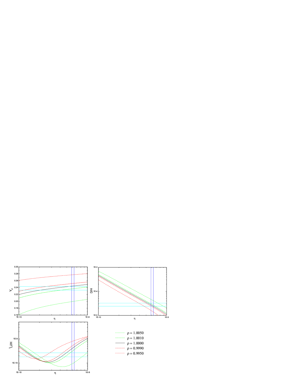
Figure 1: (color online) The primordial abundances of ${}^{4}\mathrm{He}$, D and ${}^{7}\mathrm{Li}$ as a function of the baryon-to-photon ratio $\eta$, for various values of $\rho$ as indicated by the legend in the lower right panel. Also shown are the observational allowed ranges of these abundances (the horizontal cyan lines) and the WMAP-indicated range of $\eta$ (the vertical blue lines).

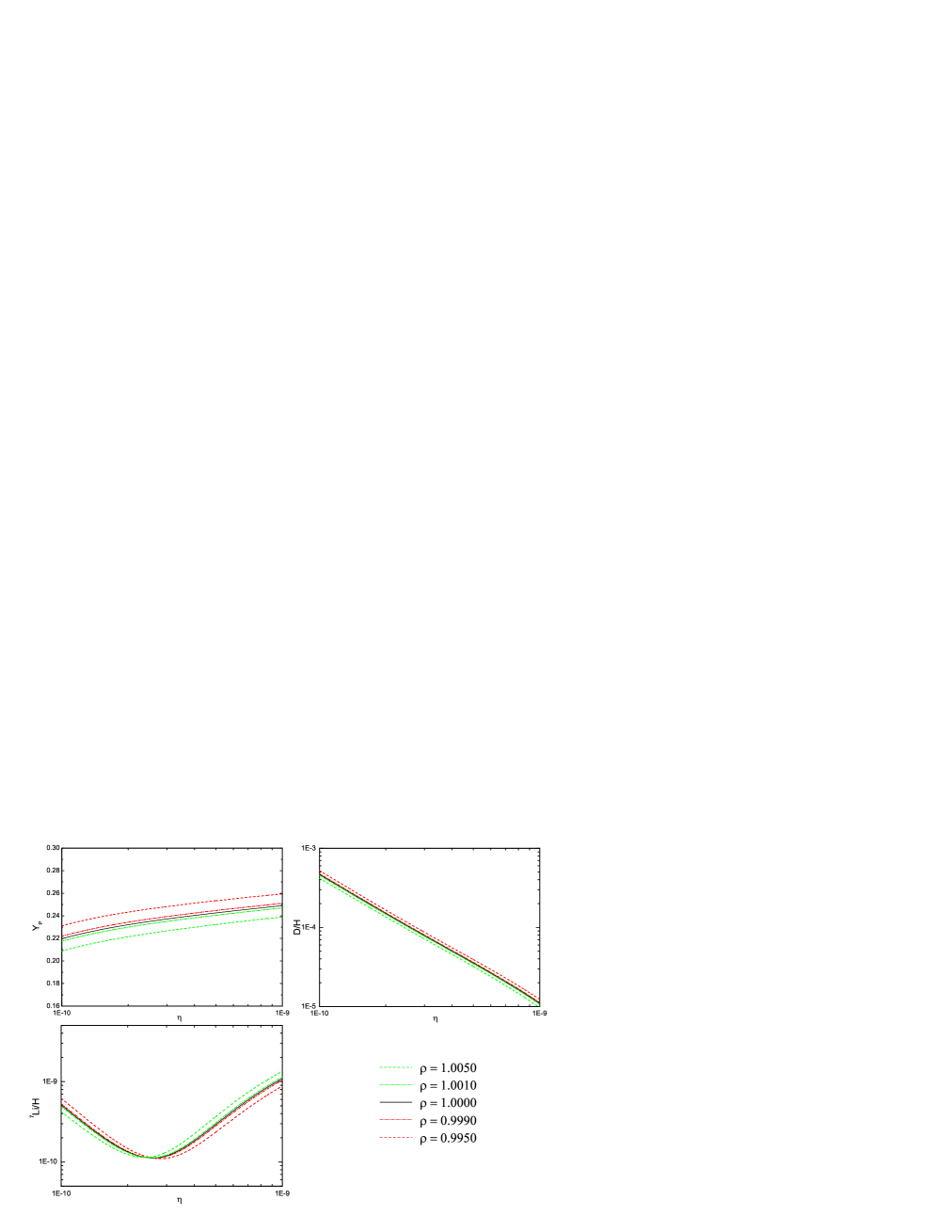
Figure 2: (color online) Similar to FIG.1, but here we neglect the effects coming from the reaction $p(n,D)\gamma$ (mainly the deuteron binding energy $B_{d}$). See the text for explanations.

With the help of Eq. (43) and the theoretical cross section for $p(n,\text{D})\gamma$, it is then straightforward to obtain the radion-dependence ($\rho$-dependence) of the thermo-averaged rate for this reaction.

For the other two neutron-induced reactions ${}^{3}\mathrm{He}(n,p){}^{3}\text{H}$ and ${}^{7}\mathrm{Be}(n,p)^{7}\mathrm{Li}$, there is no theoretical calculation like that for $p(n,\text{D})\gamma$, and so we simply use the data-fitting results and neglect their coupling dependences. The reaction ${}^{3}\mathrm{He}(n,p){}^{3}\text{H}$ influences the ${}^{3}\mathrm{He}$ output which is not used to constrain the parameters, and so the ignorance of its coupling dependences is non-essential. But the ${}^{7}\mathrm{Li}$ abundance which we use to reduce the parameter space does depend on the reaction ${}^{7}\mathrm{Be}(n,p)^{7}\mathrm{Li}$ and this reaction exhibits a broad resonance which may shift if the fundamental couplings vary; in Sec. VI we shall give a simple estimation on the error due to neglecting its coupling dependences.

V NUMERICAL RESULTS

We have incorporated all the above-discussed effects into the standard BBN code by Kawano Kawano (1992). For the nuclear reactions, we re-fit the updated rates given in the NACRE compilation NACRE (1999) (and a later work of Cyburt, Field & Olive Cyburt (2001)) in the forms as in SKM to compute the impacts of varying $\alpha_{\mathrm{EM}}$ and $\mu$. Then we compare this result with that obtained by simply using the SKM-fitted rates and find that they are essentially the same. Keeping this in mind, in the following discussions we will only use the results derived from the SKM rates.

In FIG. 1 we plot the abundances of the light nuclei ${}^{4}\mathrm{He}$, D and ${}^{7}\mathrm{Li}$ including the effects of an evolving radion field, which is characterized by the ratio between the extra space volumes at the time of BBN and at present, $\rho$. It is apparent that if the size of the extra dimensions is larger at the BBN era $(\rho>1)$, then there will be an increase in the deuterium output and decreases in the ${}^{4}\mathrm{He}$ and ${}^{7}\mathrm{Li}$ (for ${}^{7}\mathrm{Li}$ we only consider the larger-$\eta$-case in consistent with the WMAP result Spergel (2003)) yields compared with the standard BBN. The behavior of the ${}^{4}\mathrm{He}$ output is mainly the consequence of two effects originated respectively from the weak interactions and the nuclear reaction $p(n,D)\gamma$. On one hand, a $\rho$-value larger than 1 implies a smaller $\alpha_{\mathrm{EM}}$ at the time of BBN, leading to a larger $m_{np}$ (from Eq. (33)) and smaller neutron density at freeze-out, thus finally to a smaller ${}^{4}\mathrm{He}$ output (note that as discussed above, the dependence on the reduced mass $\mu$ has the same trend and strengthens this effect). Meanwhile, the weak interaction rates will be larger than those in the standard case, again decreasing the final ${}^{4}\mathrm{He}$ abundance. On the other hand, the larger $\rho$-value will cause a smaller deuteron binding energy $B_{d}$ (from Eq. (43)) than in the standard BBN, and so the nucleosynthesis will commence at a later time and become less efficient, producing less ${}^{4}\mathrm{He}$ and ${}^{7}\mathrm{Li}$ while leaving more D unprocessed (there is an extra decrease in the forward rate of $p(n,D)\gamma$ which is also due mainly to $B_{d}$, but we have checked that its influence is small compared with the effect of the later commencing BBN). Both of these two effects work in the same direction for ${}^{4}\mathrm{He}$ so that the final ${}^{4}\mathrm{He}$ yield is very sensitive to $\rho$. As for $\mathrm{D}$ and ${}^{7}\mathrm{Li}$, the effects of a larger $\rho$ other than that of $B_{d}$ come mainly from the Coulomb barrier: the charged-particle-induced reaction rates will be less suppressed since both $\alpha_{\mathrm{EM}}$ and $\mu$ are smaller in this case, consequently more $\mathrm{D}$ is processed and more ${}^{7}\mathrm{Li}$ is produced. To see this point more explicitly, we plot in FIG. 2 the BBN yields if all the effects discussed in the previous section except that of the $p(n,D)\gamma$ reaction are included. FIG.2 agrees with the trend when only the effects of changing $\alpha_{\mathrm{EM}}$ are considered, such as that in Bergstrom (1999); Ichikawa (2004). However, the inclusion of varying $B_{d}$ (as in FIG. 1) changes these abundances dramatically, indicating the important role of the deuteron binding energy in BBN Dmitriev (2004); Kneller (2003); Yoo (2003).

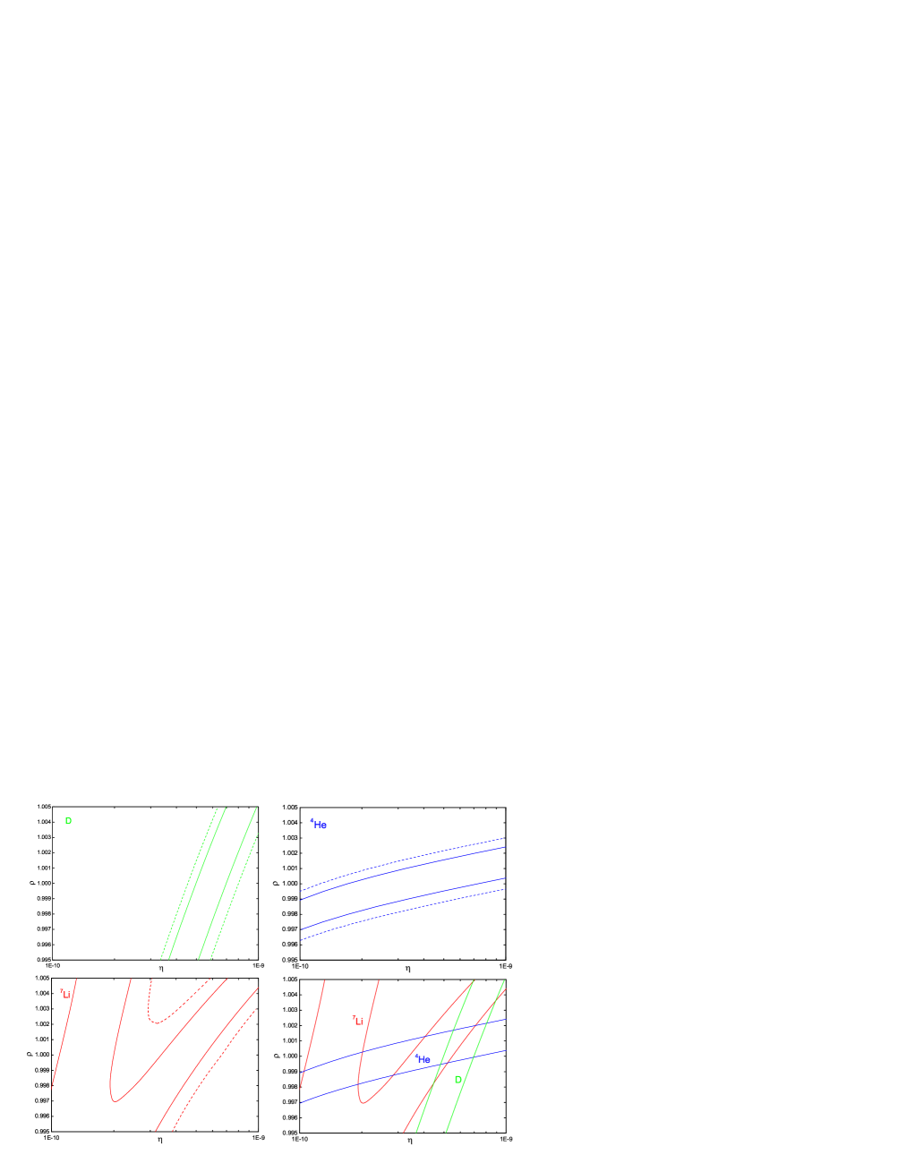
Figure 3: (color online) The 68% (solid) and 95% (dashed) contours from the observational data on D (upper left), ${}^{4}\mathrm{He}$ (upper right) and ${}^{7}\mathrm{Li}$ (lower left). The lower right panel shows the 68% contours plotted together to make the comparison explicit.

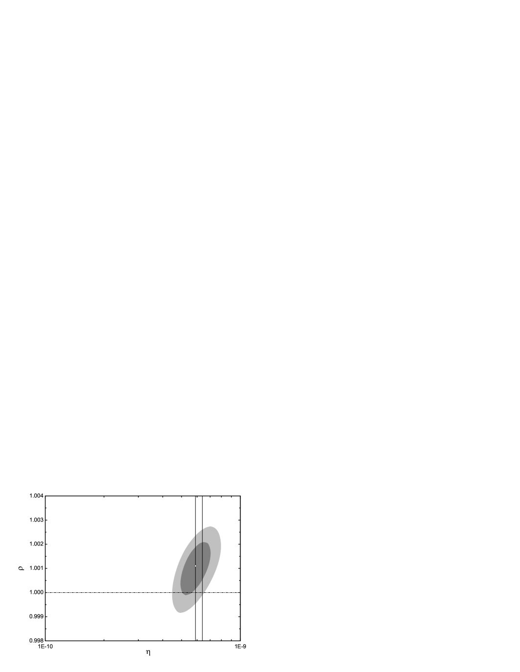
Figure 4: Joint constraint on the parameter space from $\mathrm{D}$+${}^{4}\mathrm{He}$+${}^{7}\mathrm{Li}$; the gray and light gray regions denote the 68% and 95% C. L. contours respectively. The point with the maximum likelihood, which lies around $(5.9\times 10^{-10},1.0011)$ on the $(\eta,\rho)$ plane, is also shown (the white circle). The vertical lines represent the $1\sigma$ range of $\eta$ determined by WMAP and the dot-dashed horizontal line is the case of the standard BBN $(\rho=1)$.

Our results as shown in FIG. 1 suggest that the discrepancy between the standard BBN theory and WMAP observations tends to be reduced if $\rho$ is greater than 1 Comment1 (2004). Using the WMAP-implied value of $\eta$ Spergel (2003), the standard BBN can reproduce the observed D abundance, but not the ${}^{4}\mathrm{He}$ and ${}^{7}\mathrm{Li}$ abundances; an $\eta$ smaller than the WMAP value is needed to obtain the observed ${}^{4}\mathrm{He}$ and (or) ${}^{7}\mathrm{Li}$ abundances. While this discrepancy may result from some systematic errors in the ${}^{4}\mathrm{He}$ and ${}^{7}\mathrm{Li}$ observations, the possibility of nonstandard BBN or new physics cannot be excluded. In fact, there have been many attempts of solving this discrepancy from a theoretical aspect, for example, by nonstandard expansion rate Barger (2003), varying fine structure constant Nollett (2002), and lepton asymmetry Barger (2003) etc. These effects separately cannot solve the whole inconsistency and a combination of them is needed, e.g. Ichikawa (2004) (there are also works which use a single quantity to account for the inconsistency, such as a varying deuteron binding energy Dmitriev (2004) and the Brans-Dicke cosmology with a varying $\Lambda$ term Nakamura (2005)). But from a theoretical viewpoint, such combinations may not be necessary since, as mentioned in the introduction, the variation of one fundamental constant will often be accompanied by the variations of some other constants; these changes together would play the role of several effects combined. Because the co-variation of the fundamental constants is rather model-dependent, a general study is not practical. Our present work serves as a specific example and shows how the variations of several fundamental constants are correlated with one parameter $\rho$ and driven by the same physics - in this case, the variation of the volume of extra-dimensional space.

In FIG. 1 the horizontal lines show the $1\sigma$ ranges of the measured ${}^{4}\mathrm{He}$, D and ${}^{7}\mathrm{Li}$ abundances. We use the observational results of Olive, Steigman and Walker Olive (1998) for ${}^{4}\mathrm{He}$ and the most recent work of Kirkman et al. Kirkman (2001) for D:

$$Y_{\mathrm{P}}^{\mathrm{obs}}=0.238\pm 0.005,$$ (44)

$$(\mathrm{D/H})^{\mathrm{obs}}=2.78_{-0.38}^{+0.44}\times 10^{-5}.$$ (45)

For Lithium we use the value given in the recent work of Bonifacio et al. Bonifacio (2002),

$$(^{7}\mathrm{Li}/\mathrm{H})^{\mathrm{obs}}=2.19_{-0.38}^{+0.46}\times 10^{-10},$$ (46)

which is larger than previous results but still a factor of 2 smaller than the standard BBN + WMAP result. The vertical lines in FIG. 1 represent the $1\sigma$ range of $\eta$ allowed by the CMB analysis Spergel (2003):

$$\eta_{\mathrm{WMAP}}=(6.14\pm 0.25)\times 10^{-10}.$$ (47)

In order to see to what extent the quantity $\rho$ can differ from 1, we next carry out the likelihood analysis and find the confidence contours in the two-dimensional parameter space $(\eta,\rho)$. For this purpose, we adopt the semi-analytical method introduced in Fiorentini (1998) and then slightly generalized in Cuoco (2004); Serpico (2004). The likelihood function is simply given as $L\propto\mathrm{exp}\left[-\chi^{2}/2\right]$ in which the chi-squared is calculated by:

$$\chi^{2}=\sum_{i,j}\left[Y_{i}^{\mathrm{th}}-Y_{i}^{\mathrm{obs}}\right]W_{ij}\left[Y_{j}^{\mathrm{th}}-Y_{j}^{\mathrm{obs}}\right],$$ (48)

with $W_{ij}$ the inverse covariance matrix:

$$W_{ij}=\left[\sigma_{ij}^{2,\mathrm{th}}+\sigma_{ij}^{2,\mathrm{obs}}\delta_{ij}\right]^{-1},$$ (49)

and $Y_{i}^{\mathrm{th}}$ ($Y_{i}^{\mathrm{obs}}$) are the theoretical (observational) abundances of the i-th element. In Eq. (49) $\sigma_{ij}^{2,\mathrm{th}}$ is the error matrix calculated by

$$\sigma_{ij}^{2,\mathrm{th}}=\frac{1}{4}\sum_{k}\left[Y_{i}(\Gamma_{k}^{+})-Y_{i}(\Gamma_{k}^{-})\right]\left[Y_{j}(\Gamma_{k}^{+})-Y_{j}(\Gamma_{k}^{-})\right],$$ (50)

in which $\Gamma_{k}^{+(-)}$ is the k-th nuclear reaction rate plus (minus) its $1\sigma$ uncertainty; the summation is over all the most relevant reactions. When $i=j$, Eq. (50) simply gives the theoretical uncertainty of the i-th nuclear abundance.

In FIG. 3 we show the 68% and 95% C. L. contours on the $\eta-\rho$ plane calculated using the modified Kawano code. Although neither D nor ${}^{4}\mathrm{He}$ alone could constrain the parameters considerably, we could see from the lower right panel of this figure that the combination of them reduces the allowed parameter space significantly, a similar conclusion as that in the previous works Ichikawa (2002); Yoo (2003). The WMAP-implied value of $\eta$ is seen to lie in the allowed parameter space of anyone of $\mathrm{D}$ & ${}^{4}\mathrm{He}$, $\mathrm{D}$ & ${}^{7}\mathrm{Li}$ and ${}^{4}\mathrm{He}$ & ${}^{7}\mathrm{Li}$. We have also plotted the joint constraint on the parameters from $\mathrm{D}$+${}^{4}\mathrm{He}$+${}^{7}\mathrm{Li}$ in FIG. 4 with the WMAP-implied $1\sigma$ range for $\eta$, Eq. (47), indicated by the vertical lines. It can be seen that our best fitting value (the white circle) lies just on the edge of the $1\sigma$ range of $\eta_{\mathrm{WMAP}}$ while the whole $1\sigma$ WMAP range falls into our 68% C. L. contour. On the other hand, the standard BBN $(\rho=1)$ cannot be consistent with the WMAP result and is disfavored at the 68% C. L. though it still lies inside our 95% C. L. contour. The allowed range of $\rho$ and $\eta$ by our calculation is $0.9999\lesssim\rho\lesssim 1.0021$, $4.94\times 10^{-10}\lesssim\eta\lesssim 7.05\times 10^{-10}$ at the 68% C. L. and $0.9992\lesssim\rho\lesssim 1.0027$, $4.46\times 10^{-10}\lesssim\eta\lesssim 7.99\times 10^{-10}$ at the 95% C. L., of which the ranges of $\rho$ could be transformed into the allowed variations of the fine structure constant in the present model as:

$$-2.1\times 10^{-3}(-2.7\times 10^{-3})\lesssim\frac{\alpha_{\mathrm{EM,BBN}}-\alpha_{\mathrm{EM,NOW}}}{\alpha_{\mathrm{EM,NOW}}}\lesssim 0.1\times 10^{-3}(0.8\times 10^{-3}).$$ (51)

This constraint is looser than that obtained in Ichikawa (2002) but more stringent than that in Nollett (2002).

VI DISCUSSIONS AND CONCLUSIONS

In summary, we have considered in this work the implications of a slowly evolving radion field on the fundamental constants and the Big Bang Nucleosynthesis predictions in the context of the universal extra dimensions model. We have included in our modified BBN code various effects of the varying constants, of which the most important ones being the neutron-proton mass difference, the deuteron binding energy, the free neutron lifetime and the nuclear reaction rates. These effects may act in either the same or the opposite directions and lead to distinct and complex behaviors of the light nuclei yields. We have also calculated the chi-squared as a function of $\rho$, the ratio between the extra space volumes at the time of BBN and now, and $\eta$, the baryon-to-photon ratio; this analysis then gives a bound on the variation of the fine structure constant as $-2.1\times 10^{-3}\lesssim\Delta\alpha_{\mathrm{EM}}/\alpha_{\mathrm{EM}}\lesssim 0.1\times 10^{-3}$ at 68% C. L. and $-2.7\times 10^{-3}\lesssim\Delta\alpha_{\mathrm{EM}}/\alpha_{\mathrm{EM}}\lesssim 0.8\times 10^{-3}$ at 95% C. L. The allowed range for $\Delta\alpha_{\mathrm{EM}}/\alpha_{\mathrm{EM}}$ in our result is much larger than that obtained from quasar absorption systems Murphy (2001), which is $\Delta\alpha_{\mathrm{EM}}/\alpha_{\mathrm{EM}}=(-0.72\pm 0.18)\times 10^{-5}$. However, because BBN probes physics up to redshifts of order $10^{10}$ while the quasar absorption systems are at $z=1\sim 3$, there should be no apparent inconsistency.

It is suggested that a larger extra dimension size at the time of BBN may help reduce the discrepancy between the BBN theory and observation, and here we make several comments about this conclusion. Firstly, the expression for the neutron-proton mass difference $m_{np}$ (Eq. (32)) is phenomenological but reasonable, even though it may not be definitive Bergstrom (1999); Nollett (2002); we here use it because it is the most-commonly-used and we find no competing ones. Secondly, there is an uncertainty for the parameter $r$ in the deuteron binding energy formula (Eq. (41)) derived by the effective field theory, but as we stated above, changing $r$ from 10 to 6 only induces a small variation of the numerical results while having no influence on the qualitative features we have discussed. Thirdly, our discussion on the variations of nuclear reaction rates follows that in Ichikawa (2002) and we have neglected several effects due to the lack of theoretical understandings for them. One example is the influence of a varying $B_{d}$ on the reaction rates of $\text{D}(p,\gamma){}^{3}\text{He}$, $\text{D}(\text{D},n){}^{3}\text{He}$, $\text{D}(\text{D},p){}^{3}\text{H}$, $\text{D}({}^{3}\text{H},n){}^{4}\text{He}$, $\text{D}({}^{3}\text{He},p){}^{4}\text{He}$, which are dominant or subdominant in the destruction of D. Lacking an explicit expression for this effect, we choose not to include it in the modified code. Instead we can make an estimation about the error introduced by neglecting it, by assuming the cross sections of these reactions to scale with the deuteron radius and thus $B_{d}$, i.e., $\sigma\propto 1/(m_{N}B_{d})$ Kneller (2003). Adopting this parametrization in the code, we find that the outputs of D, ${}^{4}\text{He}$ and ${}^{7}\text{Li}$ are changed by $-\lesssim 9\%$, $\lesssim 0.12\%$ and $\lesssim 5\%$ respectively in our interested range of $(\eta,\rho)$ (see FIG. 4), which lie well within the corresponding $1\sigma$ observational uncertainties ($\sim 16\%$ for D, $\sim 2\%$ for ${}^{4}\text{He}$ and $\sim 21\%$ for ${}^{7}\text{Li}$). Another example is the influence of resonances in some key cross sections such as those of $\text{D}({}^{3}\text{H},n){}^{4}\text{He}$, $\text{D}({}^{3}\text{He},p){}^{4}\text{He}$ and ${}^{7}\text{Be}(n,p){}^{7}\text{Li}$. These resonant terms are generally of the form Fowler (1967)

$$\langle\sigma|v|\rangle_{\text{res}}=F(T)\text{exp}\left[-\frac{\bar{E}}{T}\right]$$ (52)

in which $F(T)$ is a function of the temperature and $\bar{E}$ is the resonance energy. Without a reliable calculation of how these terms depend on the strong coupling, we roughly estimate the corrections from them by assuming $\bar{E}\propto\Lambda_{\text{QCD}}$. Then using the fitting values of $\bar{E}$ in these cross sections SKM (1993) in the modified code we find that the D and ${}^{7}\text{Li}$ abundances decrease by $\lesssim 0.14\%$ and $\lesssim 1.4\%$ in the same range of $(\eta,\rho)$ as above, while the ${}^{4}\text{He}$ output stays essentially unchanged. These values again fall well in the corresponding observational uncertainties. Although the points discussed in this paragraph would not change our results much, they do reflect the important role these effects play in reducing possible errors, and in any case the precisions of the BBN constraints will improve with future progress in particle and nuclear physics relevant for these topics.

It is also interesting to look at whether the allowed range for $\rho$ in our constraint would imply additional effects that are too large to be dangerous for other observations, such as the existence of bound di-proton/di-neutron and the stability of ${}^{5}\text{He}$. It is well known that the bound di-proton will open a rapid channel for the hydrogen fusion Dyson (1971) and thus be catastrophic to the star lifetimes. The binding condition for di-nucleon systems was considered by, e.g. Dent and Fairbairn Dent (2003), and a rough criterion for these systems to be stable was a decrease of $\Lambda_{\text{QCD}}$ to $\sim 1/10$ of its present day value (see Dent (2003) for more details), which is much larger than our constrained range for the gauge coupling variations. The stability of ${}^{5}\text{He}$ is also important in the consideration of varying fundamental constants as, if stable, ${}^{5}\text{He}$ would fill the mass-5 gap in the BBN nuclear reaction chain, drastically enhancing the production of ${}^{7}\text{Li}$. This issue was discussed by, e.g. Flambaum and Shuryak Flambaum (2002), and it was found there that the limit from ${}^{5}\text{He}$ binding cannot compete with that from $B_{d}$. For example, even the more stringent criterion to avoid a stable ${}^{5}\text{He}$ quoted in Ref. Flambaum (2002), namely $\delta_{\pi}\equiv\delta(m_{q}/\Lambda_{\text{QCD}})/(m_{q}/\Lambda_{\text{QCD}})\gtrsim-0.05$, is well satisfied by our $2\sigma$ range of $\rho$.

As a final point, we comment on the choices of observational ${}^{4}\text{He}$ and ${}^{7}\text{Li}$ abundances. The value given in Eq. (44) is taken from Ref. Olive (1998) and is certainly not the only observational result of $Y_{\text{P}}$. Other data analysis give different results, such as $Y^{\text{obs}}_{\text{P}}=0.2421\pm 0.0021$ in Ref. IT (2004) and $Y^{\text{obs}}_{\text{P}}=0.249\pm 0.009$ in Ref. Olive (2004). It is apparent from FIGs. 1 and 3 that, if these larger abundances are used, the ${}^{4}\text{He}$ contour will shift rightward. Meanwhile, as stated above, the ${}^{7}\text{Li}$ abundance as taken from Ref. Bonifacio (2002) is significantly larger than previous estimates such as $({}^{7}\text{Li}/\text{H})^{\text{obs}}=1.23\pm 0.06^{+0.68}_{-0.32}$ (95% C. L.) given by Ryan et al. Ryan (2000). From FIGs. 1 and 3 we see that, with the latter result adopted, the right branch of the ${}^{7}\text{Li}$ contour (which we are interested in) will shift leftward. Consequently the inconsistency between BBN and WMAP as discussed above would be less reduced.

Appendix A A FIVE DIMENSIONAL TOY MODEL OF UED

In this appendix we review briefly the main ingredients of the minimal universal extra dimension model relevant for our discussion. In particular we show that the UED model reduces to 4D SM at low temperatures. For simplicity we will assume only one extra dimension in this toy model, which is assumed to be flat and compactified on an orbifold $\mathrm{S}_{1}/\mathrm{Z}^{2}$. The fifth dimension is characterized by its coordinate $x_{4}=y\in[0,2\pi R]$, where $R$ is the radius of the fifth dimension (Note that here the convention is different from that in Section II; see Appelquist (2001) for more details).

As a minimal generalization of SM, the 5-dimensional model contains three generations of quarks and leptons, denoted by $\tilde{Q_{i}}$, $\tilde{U_{i}}$, $\tilde{D_{i}}$, $\tilde{L_{i}}$ and $\tilde{E_{i}}$ respectively where $i=1,2,3$ is the generation index (For example, the zero modes of $\tilde{Q_{1}}$, $\tilde{U_{1}}$, $\tilde{D_{1}}$, $\tilde{L_{1}}$ and $\tilde{E_{1}}$ correspond respectively to the $(u,d)_{L}$, $u_{R}$, $d_{R}$, $(\nu_{e},e^{-})_{L}$ and $e^{-}_{R}$ in the 4D SM). Then the 5-dimensional Lagrangian in the matter sector could be expressed as:

$$\tilde{L}_{5,\mathrm{total}}=\tilde{L}_{\mathrm{G}}+\tilde{L}_{\mathrm{F}}+\tilde{L}_{\mathrm{H}}+\tilde{L}_{\mathrm{Y}},$$ (53)

in which the subscripts G, F, H and Y represent the gauge, fermions, Higgs and Yukawa sectors of the model respectively and are described as:

$$\tilde{L}_{\mathrm{G}} = -\sum_{r=1}^{3}\frac{1}{2\tilde{g}_{r}^{2}}\mathrm{Tr}\left[\tilde{F}_{r}^{AB}(X)\tilde{F}_{rAB}(X)\right],$$ (54)

$$\tilde{L}_{\mathrm{F}} = i\left[\bar{\tilde{Q}}(X),\bar{\tilde{U}}(X),\bar{\tilde{D}}(X),\bar{\tilde{L}}(X),\bar{\tilde{E}}(X)\right]\times\Gamma^{A}D_{A}\left[\tilde{Q}(X),\tilde{U}(X),\tilde{D}(X),\tilde{L}(X),\tilde{E}(X)\right]^{\mathrm{T}},$$ (55)

$$\tilde{L}_{\mathrm{H}} = \left[D_{A}\tilde{H}(X)\right]^{+}D^{A}\tilde{H}(X)-\tilde{\mu}^{2}\tilde{H}^{+}(X)\tilde{H}(X)-\tilde{\lambda}\left[\tilde{H}^{+}(X)\tilde{H}(X)\right]^{2},$$ (56)

$$\tilde{L}_{\mathrm{Y}} = \tilde{Y}_{U}\bar{\tilde{Q}}(X)\tilde{U}(X)\cdot i\sigma_{2}\tilde{H}^{\ast}(X)+\tilde{Y}_{D}\bar{\tilde{Q}}(X)\tilde{D}(X)\tilde{H}(X)\tilde{Y}_{E}\bar{\tilde{L}}(X)\tilde{E}(X)\tilde{H}(X)+\mathrm{H.c.}.$$ (57)

In the above $\tilde{F}_{r}^{AB}$ denotes the 5-dimensional gauge field strength associated with the $\mathrm{SU}(3)_{\mathrm{C}}\times\mathrm{SU}(2)_{\mathrm{W}}\times\mathrm{U}(1)_{\mathrm{Y}}$ group and $D_{A}$ the corresponding covariant derivative; $\Gamma_{A}$’s are the 5-dimensional anti-commuting gamma matrices defined as $\Gamma_{A}=\{\gamma^{\mu},\gamma^{4}\}$ with $\gamma^{\mu}\ (\mu=0,1,2,3)$ being the 4D Dirac matrices and $\gamma^{4}=-i\gamma^{0}\gamma^{1}\gamma^{2}\gamma^{3}$ (for the definition of gamma matrices in more than 5 dimensions see Appelquist (2001)). As in the standard model the fermion masses are generated by the Higgs mechanism, the 5D Higgs doublet $\tilde{H}(X)$ has the same form as in 4D, $\tilde{\mu}$ and $\tilde{\lambda}$ being its potential parameters; the Yukawa couplings $Y$’s are $3\times 3$ matrices with mass dimension $-1/2$. Notice that in Eq. (A3) there is an implicit summation over the 3 generations of quarks and leptons and that the capital Latin letters A and B run from 0 to 4: $X^{A}={x^{0},x^{1},x^{2},x^{3},y}$.

In the 4-dimensional effective theory the fields could be written as an infinite summation of Kaluza Klein (KK) modes and the zero KK modes are believed to play the role of the SM particles at low energies. However, the KK expansion itself does not necessarily lead to an exact equality of the zero KK modes to SM; to obtain such an equality the KK decomposition should satisfy that, (1), only left- (right-) handed component of each weak doublet (singlet) is even under the orbifold projection and (2), the redundant zero modes of the 5th components of gauge fields, $\tilde{A}_{4}$ , should be eliminated. The KK expansions with appropriate boundary conditions which satisfy the above requirements are given as:

$$\tilde{H}(X) = \frac{1}{\sqrt{2\pi R}}\left[H^{(0)}(x)+\sqrt{2}\sum_{n=1}^{\infty}H^{(n)}(x)\mathrm{cos}\frac{ny}{R}\right],$$ (58)

$$\tilde{A_{\mu}}(X) = \frac{1}{\sqrt{2\pi R}}\left[A_{\mu}^{(0)}(x)+\sqrt{2}\sum_{n=1}^{\infty}A_{\mu}^{(n)}(x)\mathrm{cos}\frac{ny}{R}\right],$$ (59)

$$\tilde{A_{4}}(X) = \frac{1}{\sqrt{\pi R}}\sum_{n=1}^{\infty}A_{4}^{(n)}(x)\mathrm{sin}\frac{ny}{R},$$ (60)

$$\tilde{Q}(X) = \frac{1}{\sqrt{2\pi R}}\left\{Q_{L}^{(0)}(x)+\sqrt{2}\sum_{n=1}^{\infty}\left[Q_{L}^{(n)}(x)\mathrm{cos}\frac{ny}{R}+Q_{R}^{(n)}(x)\mathrm{sin}\frac{ny}{R}\right]\right\},$$ (61)

$$\tilde{U}(X) = \frac{1}{\sqrt{2\pi R}}\left\{U_{R}^{(0)}(x)+\sqrt{2}\sum_{n=1}^{\infty}\left[U_{R}^{(n)}(x)\mathrm{cos}\frac{ny}{R}+U_{L}^{(n)}(x)\mathrm{sin}\frac{ny}{R}\right]\right\},$$ (62)

$$\tilde{D}(X) = \frac{1}{\sqrt{2\pi R}}\left\{D_{R}^{(0)}(x)+\sqrt{2}\sum_{n=1}^{\infty}\left[D_{R}^{(n)}(x)\mathrm{cos}\frac{ny}{R}+D_{L}^{(n)}(x)\mathrm{sin}\frac{ny}{R}\right]\right\},$$ (63)

$$\tilde{L}(X) = \frac{1}{\sqrt{2\pi R}}\left\{L_{L}^{(0)}(x)+\sqrt{2}\sum_{n=1}^{\infty}\left[L_{L}^{(n)}(x)\mathrm{cos}\frac{ny}{R}+L_{R}^{(n)}(x)\mathrm{sin}\frac{ny}{R}\right]\right\},$$ (64)

$$\tilde{E}(X) = \frac{1}{\sqrt{2\pi R}}\left\{E_{R}^{(0)}(x)+\sqrt{2}\sum_{n=1}^{\infty}\left[E_{R}^{(n)}(x)\mathrm{cos}\frac{ny}{R}+E_{L}^{(n)}(x)\mathrm{sin}\frac{ny}{R}\right]\right\}.$$ (65)

The factor $\sqrt{2}$ above is due to the different normalizations of zero and higher order modes in the KK tower and will disappear if we run the summation over both positive and negative values of the KK numbers $n$. It’s apparent from the above decompositions that the zero modes are independent of the extra dimension coordinate $y$, a fact which is expected because the standard model should be purely 4-dimensional. The higher KK modes, however, generally depend on $y$; and they will acquire additional masses of order $n/R$, which will be accessible only with higher enough energies because of the smallness of $R$ ($1/R$ should be larger than several hundreds of GeV Appelquist (2001)). Thus up to the energy range relevant for BBN ($\mathcal{O}(1)$ MeV) the world acts as 4-dimensional and the SM description shall be safe.

Lastly let us turn to the Higgs sector of this model. The fermion masses are only generated after the spontaneous symmetry breaking (SSB); after that, the Higgs field acquires a vacuum expectation value which is determined by minimizing the Higgs potential

$$V(\tilde{H})=\tilde{\mu}^{2}\tilde{H}^{+}\tilde{H}+\tilde{\lambda}(\tilde{H}^{+}\tilde{H})^{2},$$ (66)

in which $\tilde{\mu}^{2}<0$ so that the potential has nontrivial minima Oliver (2003). In the 4D effective theory the mass of the n-th Higgs KK mode is given by $m_{H}^{(n),2}=\tilde{\mu}^{2}+n^{2}/R^{2}$. Therefore, if the size of the extra dimensions is small enough such that $|\tilde{\mu}|<1/R$, then $m_{H}^{(n),2}$ for $n\geq 1$ is positive, and only the neutral zero KK mode obtains a nonzero expectation value Oliver (2003). In this condition the zero Higgs doublet KK mode could be expanded as:

$$H^{(0)}=\left(\begin{array}[]{c}\phi^{(0)+}\\ \frac{1}{\sqrt{2}}(v+h^{(0)}+i\chi^{(0)})\\ \end{array}\right),$$ (67)

where $h^{(0)}$ is the physical Higgs zero mode $\phi^{(0)+}$ and $\chi^{(0)}$ are the zero modes of Goldstone bosons; $v$ is the (zero-mode) Higgs expectation value. At low energies as in our case, the effects of the higher order Higgs KK modes are negligible and will not be considered here.

References

- Spergel (2003) D. N. Spergel et al., Astrophy. J. Suppl. Ser. 148, 175 (2003).
- Bergstrom (1999) L. Bergström, S. Iguri and H. Rubinstein, Phys. Rev. D 60, 045005 (1999).
- Avelino (2001) P. P. Avelino et al., Phys. Rev. D 64, 103505 (2001).
- Nollett (2002) K. M. Nollett and R. E. Lopez, Phys. Rev. D 66, 063507 (2002).
- Dixit (1988) V. V. Dixit and M. Sher, Phys. Rev. D 37, 1097 (1988).
- Scherrer (1993) R. J. Scherrer and D. N. Spergel, Phys. Rev. D 47, 4774 (1993).
- Yoo (2003) J. J. Yoo and R. J. Scherrer, Phys. Rev. D 67, 043517 (2003).
- Kneller (2003) J. P. Kneller and G. C. McLaughlin, Phys. Rev. D 68, 103508 (2003).
- Flambaum (2002) V. V. Flambaum and E. V. Shuryak, Astrophys. J. 65, 103503 (2002).
- Casas (1992) J. A. Casas, J. Garcia-Bellido and N. Quiros, Mod. Phys. Lett. A 7, 447; Phys. Lett. B 278, 94 (1992).
- Serna (1992) A. Serna, R. Dominguiz-Tenreiro and G. Yepes, Astrophys. A 391, 433 (1992).
- Santiago (1997) D. I. Santiago, D. Kalligas and R. V. Wagoner, Phys. Rev. D 56, 7627 (1997).
- Damour (1999) T. Damour and B. Pichon, Phys. Rev. D 59, 123502 (1999).
- Clifton (2005) T. Clifton, J. D. Barrow and R. J. Scherrer, Phys. Rev. D 71, 123526 (2005).
- Cyburt (2003) R. H. Cyburt, B. D. Fields and K. A. Olive, Phys. Lett. B 567, 227 (2003).
- Steigman (2003) G. Steigman, hep-ph/0309347, Proceedings of the 4th International Conference on where Cosmology and Fundamental Physics Meet, Marseille, France, 23-26 June, 2003.
- Ichikawa (2004) K. Ichikawa and M. Kawasaki, Phys. Rev. D 69, 123506 (2004).
- Dmitriev (2004) V. F. Dmitriev, V. V. Flambaum and J. K. Webb, Phys. Rev. D 69, 063506 (2004).
- Webb (1999) J. K. Webb, V. V. Flambaum, C. W. Churchill, M. J. Drinkwater and J. D. Barrow, Phys. Rev. Lett. 82, 884 (1999);
- Murphy (2001) M. T. Murphy et al., Mon. Not. R. Astron. Soc. 327, 1208 (2001); ibid. 327, 1223 (2001); ibid. 327, 1237 (2001);
- Polchinski (1998) See, e.g., J. Polchinski, String Theory (Cambridge University Press, Cambridge, 1998).
- Overduin (1997) See, e.g., J. M. Overduin and P. S. Wesson, Phys. Rep. 283, 303 (1997) and references therein.
- Langacker (2002) P. Langacker, G. Segrè and M. J. Strassler, Phys. Lett. B 528, 121-128 (2002).
- Calmet (2002) X. Calmet and H. Fritzsch, Eur. Phys. J. C 24, 639-642 (2002).
- Campbell (1995) B. A. Campbell and K. A. Olive, Phys. Lett. B 345, 429-434 (1995).
- Ichikawa (2002) K. Ichikawa and M. Kawasaki, Phys. Rev. D. 65, 123511 (2002).
- Uzan (2003) J. -P. Uzan, Rev. Mod. Phys. 75, 403-450 (2003).
- ADD (1999) N. Arkani-Hamed, S. Dimopoulos and G. Dvali, Phys. Rev. D 59, 086004 (1999).
- RS (1999) L. Randall and R. Sundrum, Phys. Rev. Lett. 83, 3370 (1999); ibid. 83, 4690 (1999).
- Brax (2003) P. Brax, C. vandeBruck, A. C. Davis and C. S. Rhodes, Phys. Rev. D 67, 023512 (2003).
- Brax (2003) Ph Brax et al., Astrophys. Space Sci. 283, 627-632 (2003).
- Palma (2003) G. A. Palma, P. Brax, A. C. Davis and C. vandeBruck, Phys. Rev. D 68, 123519 (2003).
- Appelquist (2001) T. Appelquist, H. -C. Cheng and B. A. Dobrescu, Phys. Rev. D 64, 035002 (2001).
- Servant (2002) G. Servant and T. M. P. Tait, Nucl. Phys. B 650, 391-419 (2002).
- Kong (2005) K. Kong and K. T. Matchev, hep-ph/0509119.
- Kawano (1992) L. H. Kawano, FERMILAB-PUB-88/34-A (1988); FERMILAB-PUB-92/04-A (1992).
- Mazumdar (2004) A. Mazumdar, R. N. Mohapatra and A. Pérez-Lorenzana, J. Cosmo. Astro. Phys. 06, 004 (2004); we are also notified about the earlier relevant work, I. Antoniadis, Phys. Lett. B 246, 317 (1990).
- Dent (2003) T. Dent and M. Fairbairn, Nucl. Phys. B 653, 256-278 (2003);
- Dent (2003b) T. Dent, hep-ph/0305026.
- Kolb (1990) E. W. Kolb and M. S. Turner, The Early Universe (Addison-Wesley Publishing Company, 1990).
- SKM (1993) M. S. Smith, L. H. Kawano and R. A. Malaney, Astrophys. J. Suppl. Ser 85, 219-247 (1993).
- Sarkar (1996) S. Sarkar, Rep. Prog. Phys. 59, 1493-1609 (1996).
- Serpico (2004) P. D. Serpico et al., J. Cosmol. Astropart. Phys. 0412, 010 (2004); R. E. Lopez and M. S. Turner, Phys. Rev. D 59, 103502 (1999).
- PDG (2000) Particle Data Group, D. Groom et al., Eur. Phys. J. C 15, 1 (2000).
- Fowler (1964) W. A. Fowler and F. Hoyle, Astrophys. J. Suppl. No. 91 9, 201 (1964).
- Abramowitz (1964) M. Abramowitz and I. A. Stegun, Handbook of Mathematical Functions, Applied Mathematic Series, vol. 55 (Washington: National Bureau of Standards; reprinted 1968 by Dover Publications, New York).
- Fowler (1967) W. A. Fowler, G. R. Caughlan and B. A. Zimmerman, Annu. Rev. Astron. Astrophys. 5, 525 (1967); ibid. 13, 69 (1975).
- Chen (1999) J. -W. Chen and M. J. Savage, Phys. Rev. C 60, 065205 (1999).
- Rupak (2000) G. Rupak, Nucl. Phys. A 678, 405-423 (2000).
- Cyburt (2004) R. H. Cyburt, Phys. Rev. D 70, 023505 (2004).
- Epelbaum (2003) E. Epelbaum, U. -G. Meissner and W. Glockle, Nucl. Phys. A 714, 535-574 (2003).
- Beane (2003) S. R. Beane and M. J. Savage, Nucl. Phys. A 717, 91-103 (2003).
- Muller (2004) C. M. Müller, G. Schäfer and C. Wetterich, Phys. Rev. D 70, 083504 (2004).
- Gell-Mann (1968) M. Gell-Mann, R. J. Oakes and B. Renner, Phys. Rev. 175, 2195 (1968).
- Pudliner (1997) B. S. Pudliner, V. R. Pandharipande, J. Carlson, S. C. Pieper and R. B. Wiringa, Phys. Rev. C 56, 1720 (1997).
- NACRE (1999) C. Angulo et al., Nucl. Phys. A 656, 3 (1999).
- Cyburt (2001) R. H. Cyburt, B. D. Fields and K. A. Olive, New Astron. 6, 215 (2001).
- Comment1 (2004) Here we assume that by the time of CMB () all the fundamental constants take their present-day values, so we will not consider their influences on CMB. See Avelino (2001) and Yoo (2003) for effects of varying and on CMB.
- Barger (2003) V. Barger et al., Phys. Lett. B 566, 8 (2003).
- Barger (2003) V. Barger et al., Phys. Lett. B 569, 123 (2003).
- Nakamura (2005) R. Nakamura et al., astro-ph/0509076.
- Olive (1998) K. A. Olive, G. Steigman and T. P. Walker, Phys. Rep. 333, 389 (2000).
- Kirkman (2001) D. Kirkman et al., Astrophys. J. Suppl. Ser. 149, 1 (2003).
- Bonifacio (2002) P. Bonifacio et al., Astron. Astrophys. 390, 91 (2002).
- Fiorentini (1998) G. Fiorentini, E. Lisi, S. Sarkar and F. L. Villante, Phys. Rev. D 58, 063506 (1998).
- Cuoco (2004) Cuoco et al., Int. J. Mod. Phys. A 19, No. 26, 4431 (2004).
- Dyson (1971) F. Dyson, Scientific American 225 (September issue), 25 (1971).
- IT (2004) Y. I. Izotov and T. X. Thuan, Astrophys. J. 602, 200 (2004).
- Olive (2004) K. A. Olive and E. D. Skillman, Astrophys. J. 617, 29 (2004).
- Ryan (2000) S. G. Ryan, J. E. Norris and T. C. Beers, Astrophys. J. 523, 654 (1999); S. G. Ryan, T. C. Beers, K. A. Olive, B. D. Fields and J. E. Norris, Astrophys. J. Lett. 530, L57 (2000).
- Oliver (2003) See, e.g., J. F. Oliver, J. Papavassiliou and A. Santamaria, Phys. Rev. D 67, 056002 (2003).