The Effective Matter Potential for Highly Relativistic Neutrinos

Abstract

We investigate matter effects on highly relativistic neutrinos. The self-energy of neutrinos is determined in an electron or neutrino background taking into account resonance and finite width effects of the gauge bosons. We find minor changes compared to the formerly used formula for the propagator function and large deviations of the effective width from the decay width of the gauge bosons considering higher moments of the electron or neutrino distribution function.

I Introduction

In the seminal work Wolfenstein (1978), Wolfenstein explored the possibility of a change in the dynamics of neutrinos based on coherent forward-scattering with surrounding matter particles. Especially interesting is the case of a flavor sensitive charged-current background leading to a change in the neutrino oscillation probabilities. The scattering amplitude was determined using the effective four-fermion Fermi interaction. In the picture of Wolfenstein, coherent forward-scattering leads to a refractive coefficient that accordingly changes the propagation of neutrinos in a medium similar to an effective potential of strength

$$V=\sqrt{2}\,G_{F}\,(N_{e}-N_{\bar{e}}),$$ (1)

where $G_{F}$ denotes the Fermi coupling constant and $N_{e}$ and $N_{\bar{e}}$ denote the electron and positron densities of the considered medium, respectively.

Of course, this picture is not valid for arbitrarily high neutrino energies. At an energy scale $E\simeq m_{W}\approx 10^{2}\,{\rm GeV}$, where $m_{W}$ is the W-boson mass, we expect the effective Fermi theory to break down and the dynamics of the W-bosons to become important. Energies of several GeV can indeed play a role in neutrino physics, if one, e.g., considers high energetic cosmic neutrinos Lunardini and Smirnov (2001) that could be accessible by experiments. However, this estimate is premature in the sense that the kinematics of the problem has been neglected. Arguing that the energy should be of order $m_{W}$ in the center-of-mass frame, one would come to the estimate (assuming the electrons to be at rest)

$$s=2E_{\nu}\,m_{e}+m_{e}^{2}\simeq 2E_{\nu}\,m_{e}\approx m_{W}^{2},$$ (2)

where $m_{e}$ is the electron mass, which leads to

$$E_{\nu}\approx\frac{m_{W}^{2}}{2m_{e}}\approx 10^{7}\,\textrm{GeV},$$ (3)

while for scattering with another neutrino (with mass of order 1 eV)

$$E_{\nu}\approx\frac{m_{Z}^{2}}{2m_{\nu}}\approx 10^{13}\,\textrm{GeV}.$$ (4)

Indeed, taking higher-order corrections in the neutrino energy into account, one finds to next-to-leading order for relativistic neutrinos Nötzold and Raffelt (1988)

$$V=\sqrt{2}\,G_{F}\,\left[(N_{e}-N_{\bar{e}})-\frac{8\,E_{\nu}}{3m_{W}^{2}}\left(\left<E_{e}\right>N_{e}+\left<E_{\bar{e}}\right>N_{\bar{e}}\right)\right]+{\cal O}\left(\left<E_{e}^{2}\right>,\left<E_{\bar{e}}^{2}\right>\right),$$ (5)

where $\left<E_{e}\right>$ and $\left<E_{\bar{e}}\right>$ denote the average energies of the electrons and positrons in the plasma, respectively.

In this paper, we are interested in the limit of very high energetic neutrinos in matter, where the expansion used in Eq. (3) breaks down. In principle, one expects a resonance effect coming from the generation of real W-bosons by anti-neutrinos of center-of-mass energy $s\sim m_{W}^{2}$. The shape of the resonance depends on the finite decay width of the W-boson. This effect has been taken into account in Refs. Lunardini and Smirnov (2000, 2001) by the educated guess that the finite width can be represented by just including an effective propagator of the W-boson into Eq. (1), leading to

$$V=\sqrt{2}G_{F}\,\left[N_{e}\,f_{0}(-s_{W})-N_{\bar{e}}f_{0}(s_{W})\right]$$ (6)

with the propagator function given by

$$f_{0}(s_{W})=\frac{1-s_{W}}{(1-s_{W})^{2}+\gamma_{W}^{2}},$$ (7)

where $s_{W}\equiv 2E_{\nu}m_{e}/m_{W}^{2}$ and $\gamma_{W}\equiv\Gamma_{W}/m_{W}$ denotes the width of the W-boson.

The goal of this paper is to derive the propagator function from thermal field theory Le Bellac (1996); Kapusta (1993). In addition, we give arguments how a resummation of the series in Eq. (5) changes our results. In the next section, we adopt the formalism of statistical quantum field theory as it was done in Refs. Nötzold and Raffelt (1988); Pal and Pham (1989) and we present analytic as well as numerical results. Furthermore, we apply it to the cases with and without finite decay width. In a thermal background, a new energy scale enters (this scale is of order 1 keV if we consider neutrinos in the Sun up to order 1 MeV for the cosmic neutrino background at decoupling) that will change the influence of the finite decay width of the gauge boson. Finally, in Sec. III, we summarize and conclude our results.

II The Neutrino Self-Energy in a Statistical Background

In the following, we carry out the calculations for the neutrino self-energy as was done in a temperature system in Refs. Weldon (1982); Petitgirard (1992); Quimbay and Vargas-Castrillón (1995) and applied to neutrinos in an electron background in Refs. Nötzold and Raffelt (1988); Pal and Pham (1989). In contrast to these works, we expand in moments of the electron momentum $\left<p^{n}\right>$ instead of the electron energy $\left<E_{e}^{n}\right>$ what is better suited for the investigation of the resonance regime. The corresponding Feynman diagram is depicted in Fig. 1. The self-energy contributions coming from other species such as neutrinos or nuclear matter can be carried out along the same lines.

Figure 1: The Feynman diagram for the charged-current contribution to the neutrino self-energy.

In the real-time formalism, the electron propagator reads

$$S(p)=(\not{p}+m_{e})\left[\frac{1}{p^{2}-m^{2}_{e}+\textrm{i}\epsilon}+\textrm{i}\Gamma(p)\right],$$ (8)

where $\Gamma$ describes the electron background and is given by

$$\Gamma(p)=2\pi\,\delta(p^{2}-m_{e}^{2})[\theta(p^{0})n_{+}(p^{0})+\theta(-p^{0})n_{-}(-p^{0})]$$ (9)

and $n_{\pm}(p^{0})$ denote the particle distribution functions of electrons and positrons, respectively. The distribution functions are usually parameterized by the temperature and chemical potentials according to

$$n_{\pm}(p_{0})=\frac{1}{\textrm{e}^{(p_{0}-\mu_{\pm})/T}+1}.$$ (10)

Furthermore, in the unitary gauge, the W-boson propagator is given by

$$\Delta_{\mu\nu}(q)=\frac{-1}{q^{2}-m_{W}^{2}+\textrm{i}\epsilon}\left(g_{\mu\nu}-\frac{q_{\mu}q_{\nu}}{m_{W}^{2}}\right).$$ (11)

The first term in the electron propagator is the usual zero temperature ($T=0$) part, while the second term gives the following temperature contribution to the neutrino self-energy:

$$\Sigma_{T}(k) = -\frac{g^{2}}{2}\int\frac{\textrm{d}^{4}p}{(2\pi)^{3}}\,\delta(p^{2}-m_{e}^{2})[\theta(p^{0})n_{+}(p^{0})+\theta(-p^{0})n_{-}(-p^{0})]$$ (12)

$$\quad\times\gamma_{\mu}\,P_{L}\,\Delta^{\mu\nu}(k-p)\,\not{p}\gamma_{\nu}\,P_{L}\,,$$

where the weak interaction coupling constant $g$ is related to the Fermi coupling constant $G_{F}$ as $g^{2}/(8m_{W}^{2})=G_{F}/\sqrt{2}$ and $P_{L}\equiv(1-\gamma_{5})/2$ denotes the left-handed projection operator. Performing the evaluation of the Dirac algebra, this can be transformed into D’Olivo et al. (1992)

$$\Sigma_{T}(k)=-\frac{g^{2}}{2m_{W}^{2}}\left[(2m_{W}^{2}+m_{e}^{2}-k^{2})\gamma_{\mu}{\cal P}^{\mu}+2(k\cdot{\cal P}-m_{e}^{2}{\cal Q})\not{k}\right]P_{L}$$ (13)

with the definitions

$${\cal Q} = \int\frac{\textrm{d}^{4}p}{(2\pi)^{3}}[\theta(p^{0})n_{+}(p^{0})+\theta(-p^{0})n_{-}(-p^{0})]\,\frac{\delta(p^{2}-m_{e}^{2})}{(k-p)^{2}-m^{2}_{W}+\textrm{i}\epsilon},$$ (14)

$${\cal P}^{\mu} = \int\frac{\textrm{d}^{4}p}{(2\pi)^{3}}[\theta(p^{0})n_{+}(p^{0})+\theta(-p^{0})n_{-}(-p^{0})]\,\frac{p^{\mu}\delta(p^{2}-m_{e}^{2})}{(k-p)^{2}-m^{2}_{W}+\textrm{i}\epsilon}.$$ (15)

The expression ${\cal P}^{\mu}$ can be split according to

$${\cal P}^{\mu}={\cal P}_{u}u^{\mu}+{\cal P}_{k}k^{\mu},$$ (16)

where $u^{\mu}$ denotes the plasma four-vector that is $(1,0,0,0)$ in the rest frame of the plasma. The terms in the neutrino self-energy proportional to $\not{k}$ are related to the dispersion relation and the wave-function normalization and they give only corrections of order $g^{4}$ to the effective potential of the neutrinos D’Olivo et al. (1992). In what follows, we only analyze the resonance behavior of the leading-order contribution to the neutrino self-energy which translates into the following effective potential for highly relativistic neutrinos Mannheim (1988)

$$V(k)=-g^{2}\frac{2m_{W}^{2}+m_{e}^{2}-k^{2}}{2m_{W}^{2}}{\cal P}_{u}\simeq-g^{2}{\cal P}_{u}=-g^{2}\frac{k\cdot P}{k\cdot u}.$$ (17)

For simplicity, we neglect the mass (thermal and non-thermal) of the neutrino and we choose a frame such that $k=(E_{\nu},0,0,E_{\nu})$. Out of the four integrations in Eq. (12), three can be performed analytically, yielding

$$V(k) = \frac{g^{2}}{4}\int_{0}^{\infty}\frac{\textrm{d}p\,p^{2}}{2\pi^{2}E_{\nu}E_{e}}\,n_{+}(E_{e})\left[1+\frac{m_{W}^{2}-m_{e}^{2}}{4p\,E_{\nu}}\ln\left|\frac{m_{W}^{2}-m_{e}^{2}+2E_{\nu}(E_{e}-p)}{m_{W}^{2}-m_{e}^{2}+2E_{\nu}(E_{e}+p)}\right|\right]$$ (18)

$$+\,\frac{g^{2}}{4}\int_{0}^{\infty}\frac{\textrm{d}p\,p^{2}}{2\pi^{2}E_{\nu}E_{e}}\,n_{-}(E_{e})\left[1+\frac{m_{W}^{2}-m_{e}^{2}}{4p\,E_{\nu}}\ln\left|\frac{m_{W}^{2}-m_{e}^{2}-2E_{\nu}(E_{e}+p)}{m_{W}^{2}-m_{e}^{2}-2E_{\nu}(E_{e}-p)}\right|\right]$$

with $E_{e}=\sqrt{m_{e}^{2}+p^{2}}$.

First, we will reproduce the result in Eq. (5). Thus, we expand the logarithm in the loop-momentum $p$

$$\ln\left|\frac{m_{W}^{2}-m_{e}^{2}+2E_{\nu}(E_{e}\mp p)}{m_{W}^{2}-m_{e}^{2}+2E_{\nu}(E_{e}\pm p)}\right|\approx\mp\frac{4E_{\nu}p}{m_{W}^{2}-m_{e}^{2}-2E_{\nu}m_{e}}$$ (19)

and obtain

$$V(k)=\frac{g^{2}}{4}\left(\frac{N_{e}}{m_{W}^{2}-m_{e}^{2}+2E_{\nu}m_{e}}-\frac{N_{\bar{e}}}{m_{W}^{2}-m_{e}^{2}-2E_{\nu}m_{e}}\right)+{\cal O}\left(\left<p\right>\right),$$ (20)

where we have defined

$$N_{e}=\int_{0}^{\infty}\frac{\textrm{d}p\,p^{2}}{2\pi^{2}}\,\,n_{+}(E_{e}),\qquad N_{\bar{e}}=\int_{0}^{\infty}\frac{\textrm{d}p\,p^{2}}{2\pi^{2}}\,\,n_{-}(E_{e})$$ (21)

as well as

$$\left<p^{n}\right>_{e}=\frac{1}{N_{e}}\int_{0}^{\infty}\frac{\textrm{d}p\,p^{n+2}}{2\pi^{2}}\,\,n_{+}(E_{e}),\qquad\left<p^{n}\right>_{\bar{e}}=\frac{1}{N_{\bar{e}}}\int_{0}^{\infty}\frac{\textrm{d}p\,p^{n+2}}{2\pi^{2}}\,\,n_{-}(E_{e}).$$ (22)

Note that in the limit

$$\left<p^{n}\right>=0,\quad\left<E_{e}^{n}\right>=m_{e}^{n},$$ (23)

this does not reproduce the result in Eq. (5), since there is an additional contribution of order $\left<E_{e}^{-1}\right>$ that can be neglected for high temperatures which was already pointed out in LABEL:~Nötzold and Raffelt (1988). Including this contribution (and neglecting the positron background) yields

$${\cal P}_{u}=\frac{N_{e}}{m_{W}^{2}-m_{e}^{2}}\left[-\frac{1}{4}+\frac{E_{\nu}}{6(m_{W}^{2}-m_{e}^{2})}\left(4\left<E_{e}\right>-m_{e}^{2}\left<E_{e}^{-1}\right>\right)\right],$$ (24)

which agrees with our result in the considered limit.

So far, we have only expanded in the loop momentum $p$. The convergence of this expansion depends on the quotient of higher moments $\left<p^{n}\right>$ and the resonance condition appearing in the denominators

$$\frac{E^{n}_{\nu}\left<p^{n}\right>}{(m_{W}^{2}-m_{e}^{2}-2E_{\nu}m_{e})^{n}}\ll 1.$$ (25)

Hence, close to the resonance, our approximation breaks down and the divergence in Eq. (20) is removed due to the finite values of the temperature $T$ and the chemical potential $\mu$ in the electron distribution function. In Fig. 2, the full momentum dependence of the self-energy of neutrinos and anti-neutrinos is shown for the electron distribution in the Sun.

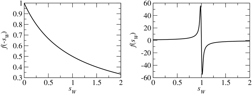
Figure 2: The propagator function $f(s_{W})$ for neutrinos (left figure) and anti-neutrinos (right figure) without finite decay width. The electron background corresponds to the properties of the Sun.

The height of the resonance can be estimated as follows. Suppose that the temperature $T$ of the distribution function is not much larger than the chemical potential $\mu$ and notice that in this case the higher-order moments behave as $\left<p^{n}\right>\sim\mu^{n}$. The potential as given in Eq. (20) then depends on the center-of-mass energy $s$ and the combination $E_{\nu}\mu/m_{W}^{2}$. Being close to the resonance and identifying this parameter with the width as in Eq. (7), we obtain the estimate

$$\gamma_{\mu}^{2}=\frac{E_{\nu}\mu}{m_{W}^{2}}\approx\frac{\mu}{2m_{e}}\approx\left(\frac{1}{30}\right)^{2}.$$ (26)

The numerical value is $\gamma_{\mu}\simeq 0.0107$, which is obtained by fitting the result with a resonance shape of the form in Eq. (7). Hence, the estimate in Eq. (26) gives the right order of magnitude.

Second, we would like to examine the inclusion of a finite width of the W-boson. The transverse and longitudinal parts of the propagator in Eq. (11) then changes to Calderón and López Castro (2001)

$$\Delta^{T}_{\mu\nu}(q) = \frac{-1}{q^{2}-m_{W}^{2}+\textrm{i}q^{2}\gamma_{W}}\left(g_{\mu\nu}-\frac{q_{\mu}q_{\nu}}{q^{2}}\right),$$ (27)

$$\Delta^{L}_{\mu\nu}(q) = \frac{1}{q^{2}-m_{W}^{2}+\textrm{i}\epsilon}\frac{q_{\mu}q_{\nu}}{q^{2}},$$ (28)

where we have defined the W-boson width as $\gamma_{W}\equiv\Gamma_{W}/m_{W}$. Using the same arguments that led us to Eq. (17), we deduce that only the term proportional to the metric $g_{\mu\nu}$ contributes to leading order and that the longitudinal part of the propagator can be neglected. Analogously to Eq. (18), we obtain

$$V(k) = \frac{g^{2}}{4}\int_{0}^{\infty}\frac{\textrm{d}p\,p^{2}}{2\pi^{2}E_{\nu}E_{e}}\,n_{+}(E_{e})\,\,\Re\left[\frac{1}{z}+\frac{m_{W}^{2}}{4p\,E_{\nu}\,z^{2}}\ln\left|\frac{m_{W}^{2}+2E_{\nu}(E_{e}-p)z}{m_{W}^{2}+2E_{\nu}(E_{e}+p)z}\right|\right]$$ (29)

$$+\,\frac{g^{2}}{4}\int_{0}^{\infty}\frac{\textrm{d}p\,p^{2}}{2\pi^{2}E_{\nu}E_{e}}\,n_{-}(E_{e})\,\Re\left[\frac{1}{z}+\frac{m_{W}^{2}}{4p\,E_{\nu}\,z^{2}}\ln\left|\frac{m_{W}^{2}-2E_{\nu}(E_{e}+p)z}{m_{W}^{2}-2E_{\nu}(E_{e}-p)z}\right|\right],$$

where we used the approximation $m_{W}^{2}-m_{e}^{2}\approx m_{W}^{2}$ and the convention $z=1+\textrm{i}\gamma_{W}$ to shorten the expression. Performing similar steps as before and neglecting higher-order corrections in the temperature and the chemical potential of the electrons, we find

$$V(k)=\sqrt{2}\,G_{F}\,(N_{e}-N_{\bar{e}})\,\Re\left[\frac{m_{W}^{2}}{m_{W}^{2}-E_{\nu}m_{e}\,z}\right],$$ (30)

or equivalently, the W-boson propagator function is given by

$$f(s_{W})=\frac{1-s_{W}}{(1-s_{W})^{2}+s_{W}^{2}\gamma_{W}^{2}}.$$ (31)

in contrast to Eq. (7). Note that, in the limit $s_{W}\to 0$, our result leads to the result of Wolfenstein, see Eq. (1), while Eq. (7) gives a correction by the factor $1/(1+\gamma_{W}^{2})$. On the other hand, in the limit $s_{W}\to\infty$, we obtain an additional factor $1/(1+\gamma_{W}^{2})$ in the effective mass of the neutrinos. This difference is due to the fact that we used a $q^{2}$-dependent damping term in Eq. (28), while a constant damping term can also be found in the literature. However, one has to have in mind that for the Standard Model value ($\gamma_{W}\simeq 0.0266$) this correction is still out of the range of experimental testability, since absorption processes become strong close to the resonance Lunardini and Smirnov (2000). On the other hand, the smallness of the width makes its influence compatible with the effect coming from finite temperature and chemical potential, cf. Eq. (26).

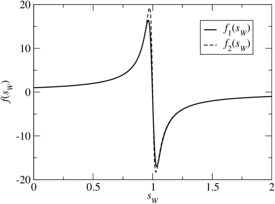
Figure 3: The propagator function $f(s_{W})$ with finite W-boson decay width. The plot $f_{1}(s_{W})$ shows the numerical result of Eq. (29) including finite temperature and chemical potential effects, corresponding to $\gamma_{\textrm{eff}}\simeq 0.0311$, while the plot $f_{2}(s_{W})$ shows the result of Eq. (31). In both cases, the electron background meets the properties of the Sun.

In Fig. 3, we have plotted the result of Eq. (31) and the full numerical result including the effects of finite temperature and chemical potential that can be obtained analogously to Eq. (18). The numerical result corresponds to an effective width of $\gamma_{\textrm{eff}}\simeq 0.0311$.

Thus, we arrive at the conclusion that in the Sun for the charged-current contributions the effect coming from the finite width of the W-boson is larger than the temperature effect, i.e., $\gamma_{\textrm{eff}}\approx\gamma_{W}\gtrsim\gamma_{\mu}$. This picture can change in different contexts. For example, in supernovae, the rather large chemical potential of the electrons leads to $\gamma_{\mu}\approx 1$, and hence, the temperature effects dominate. Similarly, this effect is important considering the scattering with the neutrino background. Due to the small neutrino masses, the resonance appears for very high neutrino energies. Thus, using Eq. (26), we obtain

$$\gamma_{\mu}^{2}=\frac{E_{\nu}\mu}{m_{W}^{2}}\approx\frac{\mu}{2m_{\nu}}$$ (32)

and the finite width from the Z-boson decay channels plays only a marginal role as long as the density of the neutrino background is larger than the mass scale of the neutrinos. This expectation is met in the numerical results of Fig. 4, where the resonance shape of the effective potential due to a neutrino background of temperature $T=10\textrm{ eV}$ is plotted for a neutrino of mass $m_{\nu}=1\,$ eV and without chemical potentials $\mu_{\pm}=0$. The resonance effect of the finite Z-width is almost completely washed-out, while the maximum of the resonance is shifted to smaller center-of-mass momentum. Since neutrinos are relativistic most of the time during the cosmological evolution (and one flavor could be relativistic even today), we expect the change of the effective width to be relevant for neutrinos from cosmic sources close to the resonance.

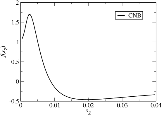
Figure 4: The propagator function $f(s_{Z})$ with finite Z-boson decay width. The plot $f(s_{Z})$ shows the numerical result of Eq. (29) including finite temperature effects ($T=10\textrm{ eV}$) of the cosmic neutrino background (CNB) of a neutrino of mass $m_{\nu}=1\,$ eV without chemical potentials $\mu_{\pm}=0$.

III Summary and Conclusion

We have analyzed the rare scenarios, where the neutrino energy is large enough such that the energy and momentum dependence of matter effects could be relevant. This is, e.g., the case for neutrinos from cosmic sources that has been analyzed in LABEL:~Lunardini and Smirnov (2001). In this limit, we have derived the shape of the resonance from thermal field theory and found a small deviation from the formerly proposed propagator function. In addition, we have examined the change in the effective width due to the finite temperature and chemical potential and found that the effective width will be much larger than the decay width of the W-boson in supernovae or the Z-boson width in the case of scattering with the relic neutrino background. Finally, we note that the Mikheyev–Smirnov–Wolfenstein (MSW) Wolfenstein (1978); Mikheyev and Smirnov (1985, 1986) resonance condition for effective mixing of neutrinos in matter will, in principle, be modified due to the temperature effects, since these effects can be interpreted as flavor conserving non-standard Hamiltonian effects Blennow et al. (2005). However, the change will be completely negligible for solar and supernova neutrinos.

References

• Wolfenstein (1978) L. Wolfenstein, Phys. Rev. D17, 2369 (1978).
• Lunardini and Smirnov (2001) C. Lunardini and A. Y. Smirnov, Phys. Rev. D64, 073006 (2001), eprint hep-ph/0012056.
• Nötzold and Raffelt (1988) D. Nötzold and G. Raffelt, Nucl. Phys. B307, 924 (1988).
• Lunardini and Smirnov (2000) C. Lunardini and A. Y. Smirnov, Nucl. Phys. B583, 260 (2000), eprint hep-ph/0002152.
• Le Bellac (1996) M. Le Bellac, Thermal Field Theory (Cambridge University Press, 1996).
• Kapusta (1993) J. Kapusta, Finite-Temperature Field Theory (Cambridge University Press, 1993).
• Pal and Pham (1989) P. B. Pal and T. N. Pham, Phys. Rev. D40, 259 (1989).
• Weldon (1982) H. A. Weldon, Phys. Rev. D26, 2789 (1982).
• Petitgirard (1992) E. Petitgirard, Z. Phys. C54, 673 (1992).
• Quimbay and Vargas-Castrillón (1995) C. Quimbay and S. Vargas-Castrillón, Nucl. Phys. B451, 265 (1995), eprint hep-ph/9504410.
• D’Olivo et al. (1992) J. C. D’Olivo, J. F. Nieves, and M. Torres, Phys. Rev. D46, 1172 (1992).
• Mannheim (1988) P. D. Mannheim, Phys. Rev. D37, 1935 (1988).
• Calderón and López Castro (2001) G. Calderón and G. López Castro (2001), eprint hep-ph/0108088.
• Mikheyev and Smirnov (1985) S. P. Mikheyev and A. Y. Smirnov, Sov. J. Nucl. Phys. 42, 913 (1985).
• Mikheyev and Smirnov (1986) S. P. Mikheyev and A. Y. Smirnov, Nuovo Cim. C9, 17 (1986).
• Blennow et al. (2005) M. Blennow, T. Ohlsson, and W. Winter (2005), eprint hep-ph/0508175.