E–WIMPs

Abstract

Extremely weakly interacting massive particles (E–WIMPs) are intriguing candidates for cold dark matter in the Universe. We review two well motivated E–WIMPs, an axino and a gravitino, and point out their cosmological and phenomenological similarities and differences, the latter of which may allow one to distinguishing them in LHC searches for supersymmetry.

1 Introduction

From the particle physics point of view, a WIMP (weakly interacting massive particle) looks rather attractive as a candidate for cold dark matter (CDM) in the Universe. In many extensions of the Standard Model (SM) there often exist several new WIMPs, and it is often not too difficult to ensure that the lightest of them is stable by means of some discrete symmetry or topological invariant. (For example, in supersymmetry, one usually invokes $R$–parity.) In order to meet stringent astrophysical constraints on exotic relics (e.g., anomalous nuclei), WIMPs must be electrically and (preferably) color neutral. They can however interact weakly. For WIMPs produced via a usual freeze–out from an expanding plasma one finds $\Omega h^{2}\simeq 1/\left\langle\left(\frac{\sigma_{\rm ann}}{10^{-38}\,\mbox{cm}^{2}}\right)\left(\frac{v/c}{0.1}\right)\right\rangle$. Assuming a pair–annihilation cross section $\sigma_{\rm ann}\sim\sigma_{\rm weak}\sim 10^{-38}\,\mbox{cm}^{2}$, and since the relative velocity $v$ at freeze–out is non–relativistic, one often obtains $\Omega h^{2}\sim 0.1$, in agreement with current determinations. This has sometimes been used as a hint for a deeper connection between weak interactions and CDM in the Universe.

Contrary to this simple and persuasive argument, CDM particles are not bound to interact with roughly the weak interaction strength. Extremely weakly interacting massive particles (E–WIMPs) have also been known to be excellent candidates for CDM. In comparison with “standard” WIMPs, E–WIMP interaction strength with ordinary matter is strongly suppressed by some large mass scale, for example the (reduced) Planck scale $M_{\rm P}\simeq 2.4\times 10^{18}\,\mbox{GeV}$ for gravitino or the Peccei–Quinn scale $f_{a}\sim 10^{11}\,\mbox{GeV}$ for axion and/or axino.

E–WIMPs are also well motivated from a particle theorist’s perspective if one takes the point of view that CDM candidates should appear naturally in some reasonable frameworks beyond the SM which have been invented to address some other major puzzle in particle physics. In other words, it would be preferable if a CDM candidate were not invented for the sole purpose of solving the DM problem.

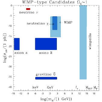
Figure 1: A schematic representation of some well–motivated WIMP–type particles for which a priori one can have $\Omega\sim 1$. $\sigma_{\rm int}$ represents a typical order of magnitude of interaction strength with ordinary matter. The neutrino provides hot DM which is disfavored. The box marked “WIMP’ stands for several possible candidates, e.g., from Kaluza–Klein scenarios.

One way to present well–motivated CDM candidates is to consider a big “drawing board” as in Fig. 1: a plane spanned by the mass of the relic on the one side and by a typical strength $\sigma_{int}$ of its interaction with ordinary matter (i.e., detectors) on the other. To a first approximation the mass range can in principle extend up to the Planck mass scale, but not above, if we are talking about elementary particles. The interaction cross section could reasonably be expected to be of the weak strength ($\sigma_{\rm weak}\simeq 10^{-2}\,\mbox{pb}$) but could also be as tiny as that purely due to gravity: $\sim\left(m_{W}/M_{\rm P}\right)^{2}\sigma_{\rm weak}\sim 10^{-32}\sigma_{\rm weak}\sim 10^{-34}\,\mbox{pb}$.

What can we put into this vast plane shown in Fig. 1? One obvious candidate is the neutrino, since we know that it exists. Neutrino oscillation experiments have basically convinced us that its mass is probably of order $\sim 0.1\,\mbox{eV}$, or less. On the upper side, if it were heavier than a few  eV, it would overclose the Universe. The problem is that such a WIMP would constitute hot DM which is hardly anybody’s favored these days. While some like it hot, or warm, most like it cold.

The main suspect for today is of course the neutralino $\chi$ jkg90 ; lrpramana03 . While in general it is a mass eigenstate of a bino, wino and two neutral higgsinos, on the grounds of naturalness lr91 or unification kkrw it should preferably be mostly a bino. LEP bounds on its mass are actually not too strong, nor robust: they depend on a number of assumptions. In minimal SUSY (the so-called MSSM) “in most cases” $m_{\chi}\mathrel{\hbox to0.0pt{\lower 4.0pt\hbox{\hskip 1.0pt$\sim$}\hss}\raise 1.0pt\hbox{$>$}}70\,\mbox{GeV}$, but the bound can be also much lower. Theoretically, because of the fine tuning argument, one expects its mass to lie in the range of several tens or hundreds of  GeV lr91 . More generally, $m_{\chi}\mathrel{\hbox to0.0pt{\lower 4.0pt\hbox{\hskip 1.0pt$\sim$}\hss}\raise 1.0pt\hbox{$>$}}{\rm few}\,\mbox{GeV}$ from $\Omega_{\chi}h^{2}\mathrel{\hbox to0.0pt{\lower 4.0pt\hbox{\hskip 1.0pt$\sim$}\hss}\raise 1.0pt\hbox{$<$}}1$ (the so–called Lee-Weinberg bound leeweinberg77 ) and $m_{\chi}\mathrel{\hbox to0.0pt{\lower 4.0pt\hbox{\hskip 1.0pt$\sim$}\hss}\raise 1.0pt\hbox{$<$}}340\,\mbox{TeV}$ from unitarity gk90 . Neutralino interaction rates are generally suppressed relative to $\sigma_{\rm weak}$ by various mixing angles in the neutralino couplings. In the MSSM they are typically between $\sim 10^{-3}\sigma_{\rm weak}$ and $\sim 10^{-10}\sigma_{\rm weak}$, although could be even lower in more complicated models where the LSP would be dominated for example by a singlino component (fermionic partner of an additional Higgs singlet under the SM gauge group). This uncertainty of the precise nature of the neutralino is reflected in Fig. 1 by showing both a smaller (dark blue) region of minimal SUSY and an extended one (light blue) with potentially suppressed interaction strengths in non–minimal SUSY models.

Another example of a WIMP that would belong to the light blue box is the the lightest Kaluza–Klein state which is massive, fairly weakly interacting and stable in some extra–dimensional frameworks st02 . One can see that a typical strength of WIMP interactions can be several orders of magnitude less then weak, while still giving $\Omega h^{2}\sim 0.1$.

Then we have E–WIMPs whose interactions are much weaker than electroweak. One well–known example is the axion – a light neutral pseudoscalar particle which is a by–product of the Peccei–Quinn solution to the strong CP problem. Its interaction with ordinary matter is suppressed by the PQ scale $\sim(m_{W}/f_{a})^{2}\sigma_{\rm weak}\sim 10^{-18}\sigma_{\rm weak}\sim 10^{-20}\,\mbox{pb}$ ($f_{a}\sim 10^{11}\,\mbox{GeV}$), hence extremely tiny, while its mass $m_{a}\sim\Lambda_{QCD}^{2}/f_{a}\sim\left(10^{-6}-10^{-4}\right)\,\mbox{eV}$ which gives $\Omega_{a}\sim 0.1$. The axion, despite being so light, is of CDM–type because it is produced by the non–thermal process of misalignment in the early Universe.

In SUSY, the axion has its fermionic superpartner, called axino. Its mass is strongly model–dependent but, in contrast to the neutralino, often not directly determined by the SUSY breaking scale $\sim 1\,\mbox{TeV}$. Hence the axino could be light and could naturally be the LSP, thus stable. An earlier study concluded that axinos could be warm DM with mass less than $2\,\mbox{keV}$ rtw90 . More recently ckr it has been pointed out more massive axinos quite naturally can be also cold DM as well, as marked in Fig. 1.

Lastly, there is the gravitino – the spin–$3/2$ superpartner of the graviton – which arises by coupling SUSY to gravity. The gravitino relic abundance can be of order one gravitinoproduction but one has to also worry about the so–called gravitino problem: heavier particles decay to gravitinos very late, around $10^{8}\sec$ after the Big Bang, and the associated energetic photons and/or hadrons may cause havoc to Big Bang Nucleosynthesis (BBN) products. The problem is not unsurmountable but more conditions/assumptions need to be satisfied as I will discuss below. In Fig. 1 the gravitino is marked in the mass range of  keV to  GeV and gravitational interactions only, although light gravitinos have actually strongly enhanced couplings via their spin–$1/2$ goldstino component.

While Fig. 1 is really about WIMPs which arise in attractive extensions of the SM, it is worth mentioning another class of relics, popularized under the name of WIMPzillas, for which there exist robust production mechanisms (curvature perturbations) in the early Universe wimpzilla:ref . As the name suggests, they are thought to be very massive, $\sim 10^{13}\,\mbox{GeV}$ or so. There are no restrictions on WIMPzilla interactions with ordinary matter, as schematically depicted in Fig. 1.

In summary, the number of well–motivated WIMP and WIMP–type candidates for CDM is in the end not so large. One can add to this picture other candidates, but the three candidates for the CDM predicted by SUSY: the neutralino, the axino and the gravitino are robust. The neutralino is testable in experimental programmes of this decade (DM searches and the LHC) and is therefore of our primary interest but we should not forget about other possibilities.

In this talk, we will discuss two intriguing E–WIMPs: the axino and the gravitino. I will demonstrate many similarities they share as well as many cosmological and phenomenological differences which may give one a chance to distinguish them from each other and from the standard neutralino at the LHC.

2 The Axino

The axino is a superpartner of the axion. It is a neutral, $R=-1$, Majorana, chiral, spin–$1/2$ particle. There exist several SUSY and supergravity implementations of the well-known original axion models (KSVZ ksvz and DFSZ dfsz ). (Axion/axino-type supermultiplets also arise in superstring models.) In studying cosmological properties of axinos, we will concentrate on KSVZ–type models where the global $U(1)$ PQ symmetry is spontaneously broken at the PQ scale $f_{a}$. A combination of astrophysical (white dwarfs, etc) and cosmological bounds leads to $10^{9}\,\mbox{GeV}\mathrel{\hbox to0.0pt{\lower 4.0pt\hbox{\hskip 1.0pt$\sim$}\hss}\raise 1.0pt\hbox{$<$}}f_{a}\sim 10^{12}\,\mbox{GeV}$axionreviews:cite although the upper bound can be significantly relaxed if inflation followed the decoupling of primordial axionic particles and the reheating temperature $T_{\rm R}\ll f_{a}$.

The two main parameters of interest to us are the axino mass and coupling. The mass $m_{\tilde{a}}$ strongly depends on an underlying model and can span a wide range, from very small ($\sim\,\mbox{eV}$) to large ($\sim\,\mbox{GeV}$) values. In contrast to the neutralino (and the gravitino), axino mass does not have to be of the order of the SUSY breaking scale in the visible sector, $M_{\rm SUSY}\sim 100\,\mbox{GeV}-1\,\mbox{TeV}$ rtw90 ; ckn . In a cosmological study of axinos, we will treat axino mass as a free parameter.

Axino couplings to other particles are generically suppressed by $1/f_{a}$. At high temperatures the most important coupling will be that of an axino–gluino–gluon dimension–five interaction term

$$i\frac{\alpha_{s}}{16\pi\left(f_{a}/N\right)}{\bar{\tilde{a}}}\gamma_{5}[\gamma^{\mu},\gamma^{\nu}]\tilde{g}^{b}F^{b}_{\mu\nu},$$ (1)

where $\tilde{g}$ stands for the gluino and $N=1(6)$ for the KSVZ (DFSZ) model. At low temperatures, on the other hand, often a dominant role will be played by an analogous coupling of axino–photon–neutralino

$$i\frac{\alpha_{Y}C_{aYY}}{16\pi\left(f_{a}/N\right)}{\bar{\tilde{a}}}\gamma_{5}[\gamma^{\mu},\gamma^{\nu}]\widetilde{B}B_{\mu\nu},$$ (2)

where $\widetilde{B}$ denotes the bino, the fermionic partner of the $U(1)_{Y}$ gauge boson $B$, which is one of the components of the neutralino. Depending on a model, there are also terms involving dimension–four operators coming, e.g., from the effective superpotential $\Phi\Psi\Psi$ where $\Psi$ is one of MSSM matter (super)fields. Axino production processes coming from such terms will be suppressed at high energies relative to processes involving Eq. (1) and (2) by a factor $m_{\Psi}^{2}/s$ where $s$ is the square of the center of mass energy. Such terms will play an important role in axino production from squark and slepton decays at low temperatures.

Axino Production

Because axino interactions are strongly suppressed, their initial thermal population decouples at very high temperatures. We further assume that it (and those of other relics, like gravitinos) present in the early Universe was subsequently diluted away by inflation and that $T_{\rm R}<T_{\rm D}$. It also had to be less than $f_{a}$, otherwise the PQ would have been restored thus leading to the well-known domain wall problem associated with global symmetries.

There are two generic ways of repopulating the Universe with axinos. First, they can be generated through thermal production (TP), via scatterings and decay processes of ordinary particles and sparticles in thermal bath. Second, they may also be produced in decay processes of particles which themselves are out–of–equilibrium, in non thermal production (NTP). These production mechanisms will also apply to the gravitino E–WIMP.

Thermal Production

The thermal production can be obtained by integrating the Boltzmann equation with both scatterings and decays of particles in the plasma.

The main axino production channels are the scatterings of (s)particles described by a dimension–five axino-gaugino-gauge boson term, Eq. (1). Because of the relative strength of $\alpha_{s}$, the most important contributions will come from 2–body strongly interacting processes into final states, $i+j\rightarrow\tilde{a}+\cdots$.

Axinos can also be produced through decays of heavier superpartners in thermal plasma. At $T\mathrel{\hbox to0.0pt{\lower 4.0pt\hbox{\hskip 1.0pt$\sim$}\hss}\raise 1.0pt\hbox{$>$}}m_{\tilde{g}}$ these are dominated by the decays of gluinos into LSP axinos and gluons. At lower temperatures $m_{\chi}\mathrel{\hbox to0.0pt{\lower 4.0pt\hbox{\hskip 1.0pt$\sim$}\hss}\raise 1.0pt\hbox{$<$}}T\mathrel{\hbox to0.0pt{\lower 4.0pt\hbox{\hskip 1.0pt$\sim$}\hss}\raise 1.0pt\hbox{$<$}}m_{\tilde{g}}$, neutralino decays to axinos also contribute while at higher temperatures they are sub–dominant. The TP contribution to axino abundance will be denoted by $\Omega^{\rm TP}_{\tilde{a}}h^{2}$.

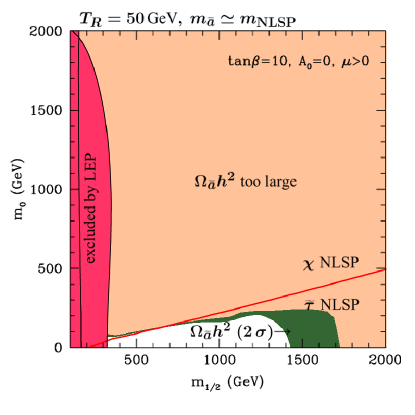
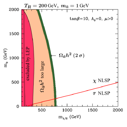
Figure 2: The plane ($m_{1/2},m_{0}$) for axino only slightly less massive than the NLSP and $T_{\rm R}=50\,\mbox{GeV}$ (left window) and for $m_{\tilde{a}}=1\,\mbox{TeV}$ and $T_{\rm R}=200\,\mbox{GeV}$ (right window). We take $\tan\beta=10$, $A_{0}=0$, $\mu>0$ and $f_{a}=10^{11}\,\mbox{GeV}$. The regions excluded by LEP are shown in red. The dark green (orange, white) regions correspond to $0.094<\Omega_{\tilde{a}}h^{2}<0.129$ ($\Omega_{\tilde{a}}h^{2}$ too large and excluded, too small but otherwise allowed) The red line divides the neutralino and stau NLSP regions.

Non-Thermal Production

As the Universe cools down, all heavier SUSY partners will first cascade decay to the next–to–lightest superpartner (NLSP), which we denote by $X$. The NLSPs then freeze out of thermal equilibrium and subsequently decay into axinos (or gravitinos).

For example, when the NLSP is a nearly pure bino ($X\simeq\widetilde{B}$), the decay time is approximately given by ckr ; ckkr

$$\begin{split}\tau(X\rightarrow\tilde{a}\,\gamma)\simeq 0.3\sec\left(\frac{100\,\mbox{GeV}}{m_{X}}\right)^{3}\ldots\end{split}$$ (3)

which means that the decay will mostly take place before the epoch of BBN and an energetic photon produced along the axino will not do any harm to light elements. This is very different from the gravitino case which is produced long after BBN.

Since all the NLSPs subsequently decay into axinos, the axino abundance $\Omega^{\rm NTP}_{\tilde{a}}h^{2}$ from NLSP decay can be determined by the simple relation of mass ratio and NLSP abundance $\Omega_{X}$,

$$\Omega_{\tilde{a}}^{NTP}=\frac{m_{\tilde{a}}}{m_{X}}\Omega_{X}.$$ (4)

Axino LSP in the CMSSM

From now on we’ll concentrate on the Constrained Minimal Supersymmetric Standard Model (CMSSM) kkrw in which all the Higgs and superpartner mass spectra are parametrized in terms of a common gaugino $m_{1/2}$ and scalar $m_{0}$ mass parameters, a common trilinear parameter $A_{0}$ (all defined at the GUT scale), as well as the ratio of the vev’s of the two Higgs doublets $\tan\beta$. The CMSSM is a reasonable low–energy framework for many GUT–based models and is also of experimental interest as a benchmark model for the LHC.

In the CMSSM, the NLSP is typically either the (bino–dominated) neutralino $\chi$ (for $m_{1/2}\ll m_{0}$) or the lighter stau ${\tilde{\tau}}_{1}$ (for $m_{1/2}\gg m_{0}$). It can decay to the axino and photon $\chi\rightarrow\tilde{a}\gamma$ or via ${\tilde{\tau}}_{1}\rightarrow\tilde{a}\tau$.

Below we illustrate axino LSP as CDM with two examples taken from Ref. crs ; crrs . In Fig. 2, the ($m_{1/2},m_{0}$) plane is shown for $\tan\beta=10$ and for $T_{\rm R}=50\,\mbox{GeV}$, $m_{\tilde{a}}\simeq m_{NLSP}$ (left window) and $T_{\rm R}=200\,\mbox{GeV}$, $m_{\tilde{a}}=1\,\mbox{GeV}$ (right window). We apply several constraints from colliders: the lower mass bounds on chargino $m_{\chi^{\pm}}>104\,\mbox{GeV}$, Higgs $m_{h}>114.4\,\mbox{GeV}$ and stau $m_{{\tilde{\tau}}_{1}}>87\,\mbox{GeV}$ at LEP and from $BR(B\rightarrow X_{s}\gamma)=(3.34\pm 0.68)\times 10^{-4}$. In addition, the orange colored region is excluded by the overclosure of Universe while the white regions are cosmologically allowed but not favored. The (green) band between the orange and white regions is the cosmologically favored ($2\,\sigma$) region of $\Omega_{\tilde{a}}h^{2}=\Omega^{\rm TP}_{\tilde{a}}h^{2}+\Omega^{\rm NTP}_{\tilde{a}}h^{2}$ consistent with observations. The recent WMAP results combined with other measurements imply the $2\,\sigma$ range for non-baryonic CDM $0.094<\Omega_{{\rm CDM}}h^{2}<0.129$ wmap_cdm .

In the left window NTP plays a dominant role. We have chosen the axino mass as large as possible (slightly lighter than NLSP). Almost all the neutralino NLSP region is excluded by an over–abundance of CDM except for tiny region of small $m_{1/2}$ and $m_{0}$. (This case is nearly identical to the standard case of neutralino LSP.) A cosmologically favored region mostly lies in the stau NLSP regime.

In the right window, where we have chosen a small axino mass, the dominant contribution comes from TP and the overall pattern of cosmologically excluded and allowed regions is very different. In particular, the region closer to the $m_{0}$ axis is excluded. As $T_{\rm R}$ increases, it grows and pushes away the green band of the cosmologically favored region farther to the right. Since, due to the small $m_{\tilde{a}}$, NTP is negligible, the band of $\Omega_{\tilde{a}}h^{2}\sim 0.1$ extends to both the neutralino and the stau NLSP regions.

In both windows one finds that the cosmologically favored region lies in the stau NLSP region (below red line), which is traditionally believed to be excluded as corresponding to a stable charged relics.

Note also a rather low $T_{R}$. In fact, this is a characteristic feature of axino CDM scenario ckr ; ckkr ; crs ; crrs where NTP allows for $T_{\rm R}\mathrel{\hbox to0.0pt{\lower 4.0pt\hbox{\hskip 1.0pt$\sim$}\hss}\raise 1.0pt\hbox{$<$}}10^{4}\,\mbox{GeV}$ and TP for somewhat larger values $\mathrel{\hbox to0.0pt{\lower 4.0pt\hbox{\hskip 1.0pt$\sim$}\hss}\raise 1.0pt\hbox{$<$}}10^{6}\,\mbox{GeV}$.

3 THE GRAVITINO

Let us now examine the gravitino as the true LSP and a candidate for CDM. Its mass arises through the super–Higgs mechanism and in a gravity–mediated SUSY breaking case is naturally expected in the range $m_{\widetilde{G}}\sim\,\mbox{GeV}-\,\mbox{TeV}$. In other SUSY breaking scenarios it can be much smaller or larger. As before with the axino, here we will take the gravitino mass to be a free parameter.

The gravitino can be produced in very much the same way as the axino, via TP and NTP. One crucial difference is that, relative to Eqs. (1) and (2), in the denominators of analogous dimension–five and four terms there appears a square of the gravitino mass $m_{\widetilde{G}}$, in addition to $f_{a}/N\rightarrow M_{\rm P}$. This leads to a different dependence of the gravitino yield on $m_{\widetilde{G}}$. In particular, after integrating the Boltzmann equation, for the TP part one finds bbp98 ; bbb00

$$\Omega^{\rm TP}_{\widetilde{G}}h^{2}\simeq 0.2\left(\frac{T_{\rm R}}{10^{10}\,\mbox{GeV}}\right)\left(\frac{100\,\mbox{GeV}}{m_{\widetilde{G}}}\right)\left(\frac{m_{\tilde{g}}(\mu)}{1\,\mbox{TeV}}\right)^{2},$$ (5)

where $m_{\tilde{g}}(\mu)$ above is the running gluino mass. One can see that, for natural ranges of $m_{\tilde{g}}$ and $m_{\widetilde{G}}$, one can have $\Omega^{\rm TP}_{\widetilde{G}}h^{2}\sim 0.1$ at $T_{\rm R}$ as high as $10^{9-10}\,\mbox{GeV}$.

For NTP production, on the other hand, one simply replaces $m_{\tilde{a}}\rightarrow m_{\widetilde{G}}$ in Eq. (4). NLSP first freeze out and then decay into gravitinos at late times which strongly depend on the NLSP composition and mass $m_{X}$, and on the decay products feng03-prl ; eoss03-grav . The lifetime is roughly given by

$$\tau_{X}\sim 10^{8}\sec\left(\frac{100\,\mbox{GeV}}{m_{X}}\right)^{5}\left(\frac{m_{\widetilde{G}}}{100\,\mbox{GeV}}\right)^{2}$$ (6)

for $m_{\widetilde{G}}\ll m_{X}$. Thus in the parameter space allowed by other constraints it can vary from from $\mathrel{\hbox to0.0pt{\lower 4.0pt\hbox{\hskip 1.0pt$\sim$}\hss}\raise 1.0pt\hbox{$>$}}10^{8}\sec$ at smaller $m_{X}$ down to $10^{2}\sec$, or even less, for large $m_{1/2}$ and/or $m_{0}$ in the  TeV range. This happens during or after BBN, which gives a strong constraints on the gravitino LSP scenario.

In Fig. 3 we display the ($m_{1/2},m_{0}$) plane (now on a log–log scale) for two representative choices: $\tan\beta=10$ and $m_{\widetilde{G}}=m_{0}$ (left window) and $\tan\beta=50$ and $m_{\widetilde{G}}=0.2m_{0}$ (right window), and for $A_{0}=0$ and $\mu>0$. In addition to the regions excluded by LEP (on the left), we also reject those where the gravitino is not the LSP or where some sparticles become tachyonic, as in the right window. The total gravitino abundance (NTP+TP) consistent with WMAP is shown in dark green region. The right and upper region of the band is cosmologically excluded from the over–abundance of DM. The light green region (marked “NTP”) corresponds to the case when NTP alone is considered, which is dominant at low $T_{R}$.

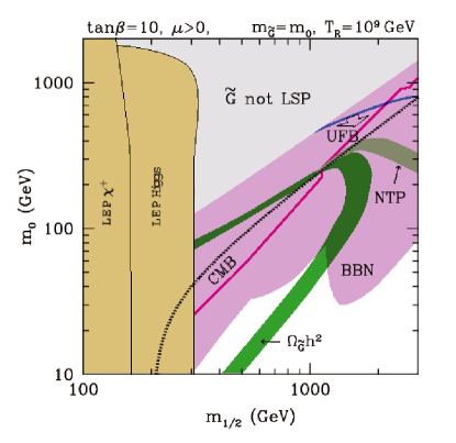
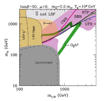
Figure 3: The plane ($m_{1/2},m_{0}$) for $\tan\beta=10$ (left window) and $\tan\beta=50$ (right window) and for $A_{0}=0$ and $\mu>0$. The light brown regions labelled “LEP $\chi^{+}$” and “LEP Higgs” are excluded by unsuccessful chargino and Higgs searches at LEP, respectively. In the right window the darker brown regions labelled “$b\to s\gamma$” is excluded assuming minimal flavor violation and the dark grey region below the dashed line is labelled “TACHYONIC” because of some sfermion masses becoming tachyonic and is also excluded. In the rest of the grey region (above the dashed line) the stau mass bound $m_{{\tilde{\tau}}_{1}}>87\,\mbox{GeV}$ is violated. In both windows, the dark green bands labelled “$\Omega_{\widetilde{G}}h^{2}$” denote the total relic abundance of the gravitino from both thermal and non–thermal production is in the favored range, while in the light green regions (marked “NTP”) the same is the case for the relic abundance from NTP processes alone. The regions excluded by the various BBN constraint are denoted in violet. A solid magenta curve labelled “CMB” delineates the region (on the side of label) inconsistent with the CMB spectrum. The UFB constraints disfavor all the stau NLSP region that has remained allowed after applying the BBN and CMB constraints.

BBN constraints

The $\chi$ NLSP decays predominantly to photons via $\chi\rightarrow\widetilde{G}+\gamma$ and (in a small fraction) to hadrons $\chi\rightarrow\widetilde{G}\gamma^{\ast}/Z^{\ast}\rightarrow\widetilde{G}q\bar{q}$. For the ${\tilde{\tau}}_{1}$ NLSP, the dominant mode is ${\tilde{\tau}}_{1}\rightarrow\widetilde{G}\tau$ and hadronic jets are produced by 4–body decays with suppressed branching ratio. However if kinematically allowed, higher hadronic branching ratio can be obtained through subsequent $Z/$Higgs bosons decays after NLSP decay to them.

The decay products, such as photons (tau leptons for $\tilde{\tau}$ NLSP) and hadrons, carry high energies inherited from the parent NLSP. These energetic particles may change the abundances of light elements produced during the epoch of BBN thus spoiling a good agreement of light element abundances between predictions and observations.

The injection of high energy photons (or charged leptons) at late times ($\tau\gtrsim 10^{4}\sec$) can disintegrate $D$ (for $\tau\lesssim 10^{6}\sec$) and ${}^{4}He$ (for $\tau\gtrsim 10^{6}\sec$) leading to the production of other lighter elements, such as $D$, ${{}^{3}}{\!He}$ or ${{}^{6}}{\!Li}$.

At earlier times ($\tau\lesssim 10^{4}\sec$) hadronic showers are induced by mesons for $\tau\lesssim 10^{2}\sec$ and nucleons for $\tau\gtrsim 10^{2}\sec$. Mesons convert protons to neutrons resulting in an increase of ${}^{4}He$ abundance, and nucleons increase the abundance of $D$ and ${}^{6}Li$.

We calculate the light element abundances in a self–consistent way using a code in jedamzik04 and compare them with observations. Here we adopt the conservative abundances of light elements,

$2.2\times 10^{-5}<$	$D/H$	$<5.3\times 10^{-5}$
$0.232<$	$Y_{p}$	$<0.258$
$8\times 10^{-11}<$	${{}^{7}}{\!Li}/H$
	${{}^{3}}{\!He}/D$	$<1.72$
	${{}^{6}}{\!Li}/{{}^{7}}{\!Li}$	$<0.1875$.

In Fig. 3 the regions excluded by constraints from light element abundances are shown in violet and marked “BBN”. We can see that the neutralino NLSP region is not viable fst04 while large parts of the stau NLSP domain are, and this is also where the total gravitino relic abundance in the range consistent with WMAP. On the other hand, the (light green) region of NTP only is not consistent with BBN. Thus a substantial contribution from TP, and therefore a large enough $T_{\rm R}$ is required. On the other hand, increasing $T_{\rm R}$ causes the green band of $\Omega_{\widetilde{G}}h^{2}$ to move to the left, which eventually runs into conflict with BBN. In the moderate gravitino mass region we could find a reheating temperature as high as $T_{R}\lesssim 4\times 10^{9}\,\mbox{GeV}$ consistent with all other constraints.

CMB constraints

The radiative decay process of NLSP releases a net photon energy into the electromagnetic plasma. For late decays, number changing interactions, such as thermal bremsstrahlung and double Compton scattering, may be ineffective, resulting in a discrepancy with Planckian distribution hu93 . The observed Planckian shape of CMB gives the constraints on the upper bound of a dimensionless chemical potential $\mu$, $|\mu|<9\times 10^{-5}$ mubound . For later decays ($\tau\gtrsim 4\times 10^{11}\simeq 8.8\times 10^{9}\sec$) constraints on CMB can be described by the Compton parameter $y$ where $|y|<1.2\times 10^{-5}$ pdg02 .

A magenta line in Fig. 3 delineates the region inconsistent with CMB spectrum. We find that the CMB constraints is usually less stringent than the constraints from the BBN.

False vacuua

The presence of scalars with color and electric charge in SUSY theories induce a possible existence of charge and color breaking (CCB) minima. Also along some directions in field space the potential can even become unbounded from below (UFB) at tree level. (After including one loop corrections a UFB direction develops a deep CCB minimum.) The most dangerous one is the UFB–3 direction involving the scalar fields $\{H_{u},\nu_{L_{i}},e_{L_{j}},e_{R_{j}}\}$ with $i\neq j$ clm1 . By simple analytical minimization of relevant terms of the scalar potential and requiring $V_{\rm UFB-3}(Q=\hat{Q})>V_{\rm Fermi}$, where $\hat{Q}$ is the minimization scale and $V_{\rm Fermi}$ is the Fermi minimum evaluated at the typical scale of SUSY masses, one obtains a constraint on the SUSY parameter space.

In Fig. 3, regions corresponding to our vacuum being a false vacuum are delineated by a blue line (on the side of a big arrow) and marked “UFB”. We can see that the constraint disfavors almost all of the stau NLSP region. (Note that this bound is not specific to the gravitino and applies to the axino case as well.) However, the existence of such a dangerous global vacuum cannot be excluded since the color and electric neutral Fermi vacuum which the Universe is in may be a long–lived local minimum. In this case a non-trivial constraints is placed on the inflationary cosmology fors95 ; forss96 .

4 Conclusions

E–WIMPs are well motivated, attractive and intriguing candidates for CDM. Here we have presented two cases of the axino and the gravitino as stable relics and CDM in the Universe. In the CMSSM, while the neutralino and stau NLSP remain allowed for the axino LSP, for GeV gravitino LSP the neutralino NLSP is excluded and only the stau NLSP remains allowed. In the stau region our vacuum corresponds to a local minimum while in the global one color and/or electric charge are not conserved. This is one lesson that we can learn should at the LHC a massive, electrically charged particle (the stau) be observed as an effectively stable state, rather then the neutralino. If enough of them were accumulated, one could possibly observe their decays and very different differential event distributions bchrs05 could, at least in some cases, allow one to decide whether Nature has chosen the axino or the gravitino as a stable relic and cold dark matter in the Universe.

References

- (1) G. Jungman, M. Kamionkowski and K. Griest, Phys. Rept. 267 (1996) 195.
- (2) For a recent review, see, e.g., L. Roszkowski, Pramana 62 (2004) 389 [hep-ph/0404052].
- (3) L. Roszkowski, Phys. Lett. B 262 (1991) 59.
- (4) G.L. Kane, C. Kolda, L. Roszkowski and J.D. Wells, Phys. Rev. D 49 (1994) 6173.
- (5) B.W. Lee and S. Weinberg, Phys. Rev. Lett. 39 (1977) 165. See also E.W. Kolb and M.S. Turner, The Early Universe, Addison-Wesley, Redwood City, 1990.
- (6) K. Griest and M. Kamionkowski, Phys. Rev. Lett. 64 (1990) 615.
- (7) G. Servant and T. Tait, Nucl. Phys. B 650 (2003) 391 and New J. Phys. 4 (2002) 99; D. Hooper and G.D. Kribs, Phys. Rev. D 67 (2003) 055003.
- (8) K. Rajagopal, M.S. Turner and F. Wilczek, Nucl. Phys. B 358 (1991) 447.
- (9) L. Covi, J.E. Kim and L. Roszkowski, Phys. Rev. Lett. 82 (1999) 4180 [arXiv:hep-ph/9905212].
- (10) L. Covi, H.B. Kim, J.E. Kim and L. Roszkowski, J. High Energy Phys. 0105 (2001) 033 [arXiv:hep-ph/0101009].
- (11) H. Pagels and J.R. Primack, Phys. Rev. Lett. 48 (1982) 223; S. Weinberg, Phys. Rev. Lett. 48 (1982) 1303; J. Ellis, A.D. Linde and D.V. Nanopoulos, Phys. Lett. B 118 (1982) 59; Phys. Lett. B 443 (1998) 209; and several more recent papers.
- (12) D.J.H. Chung, E.W. Kolb and A. Riotto, Phys. Rev. Lett. 81 (1998) 4048; V. Kuzmin and I. Tkachev, Phys. Rev. D 59 (1999) 123006.
- (13) J. E. Kim, Phys. Rev. Lett. 43 (1979) 103; M. A. Shifman, V. I. Vainstein and V. I. Zakharov, Nucl. Phys. B 166 (1980) 4933.
- (14) M. Dine, W. Fischler and M. Srednicki, Phys. Lett. B 104 (1981) 99; A. P. Zhitnitskii, Sov. J. Nucl. Phys. 31 (1980) 260.
- (15) J.E. Kim, Phys. Rept. 150 (1) 1987; M.S. Turner, Phys. Rept. 197 (67) 1990; P. Sikivie, Nucl. Phys. 87 (Proc. Suppl.) (2000) 41.
- (16) E.J. Chun, J.E. Kim and H.P. Nilles, Phys. Lett. B 287 (123) 1992.
- (17) L. Covi, L. Roszkowski and M. Small, J. High Energy Phys. 0207 (2002) 023 [hep-ph/0206119].
- (18) L. Covi, L. Roszkowski, R. Ruiz de Austri and M. Small, J. High Energy Phys. 0406 (2004) 003 [hep-ph/0402240].
- (19) D.N. Spergel, et al., Astrophys. J. Suppl. 148 (2003) 175.
- (20) L. Roszkowski, R. Ruiz de Austri and K.-Y. Choi, J. High Energy Phys. 0508 (2005) 080 [hep-ph/0408227].
- (21) D.G. Cerdeño, K.-Y. Choi, K. Jedamzik, L. Roszkowski and R. Ruiz de Austri, hep-ph/0509275.
- (22) M. Bolz, W. Buchmüller and Plümacher, Phys. Lett. B 443 (1998) 209 [hep-ph/9809381].
- (23) M. Bolz, A. Brandenburg and W. Buchmüller, Nucl. Phys. B 606 (2001) 518 [hep-ph/0012052].
- (24) J.L. Feng, A. Rajaraman and F. Takayama, Phys. Rev. Lett. 91 (2003) 011302 [arXiv:hep-ph/0302215].
- (25) J. Ellis, K.A. Olive, Y. Santoso and V. Spanos, Phys. Lett. B 588 (2004) 7 [hep-ph/0312262].
- (26) K. Jedamzik, Phys. Rev. D 70 (2004) 063524 [astro-ph/0402344].
- (27) J.L. Feng, S. Su and F. Takayama, Phys. Rev. D 70 (2004) 063514 [hep-ph/0404198] and Phys. Rev. D 70 (2004) 075019 [hep-ph/0404231].
- (28) W. Hu and J. Silk, Phys. Rev. Lett. 70 (1993) 2661 and Phys. Rev. D 48 (1993) 485.
- (29) D.J. Fixsen, et al., Astrophys. J. 473 (1996) 576; K. Hagiwara, et al., [Particle Data Group], Phys. Rev. D 66 (2002) 010001.
- (30) K. Hagiwara, et al., Phys. Rev. D 66 (2002) 010001.
- (31) J.A. Casas, A. Lleyda and C. Muñoz, Nucl. Phys. B 471 (1996) 3.
- (32) T. Falk, K.A. Olive, L. Roszkowski, M. Srednicki, Phys. Lett. B 367 (1996) 183.
- (33) T. Falk, K.A. Olive, L. Roszkowski, A. Singh, M. Srednicki Phys. Lett. B 396 (1997) 50.
- (34) A. Brandenburg, L. Covi, K. Hamaguchi, L. Roszkowski and F.D. Steffen, Phys. Lett. B 617 (2005) 99 [hep-ph/0501287].