CPHT-RR-060.1005

LPT-ORSAY-05-70

Saclay T05/167

hep-ph/0511001

Classical running of neutrino masses
from six dimensions

E. Dudas^a,b, C. Grojean^c, S.K. Vempati^a

^a Centre de Physique Theorique, Ecole Polytechnique, 91128 Palaiseau Cedex, France

^b LPT, Bât. 210, Univ. de Paris-Sud, F-91405 Orsay, France

^c Service de Physique Théorique, CEA Saclay, F91191 Gif–sur–Yvette, France
Emilian.Dudas@cpht.polytechnique.fr, grojean@spht.saclay.cea.fr, vempati@cpht.polytechnique.fr

We discuss a six dimensional mass generation for the neutrinos. Active neutrinos live on a three-brane and interact via a brane localized mass term with a bulk six-dimensional standard model singlet (sterile) Weyl fermion, the two dimensions being transverse to the three-brane. We derive the physical neutrino mass spectrum and show that the active neutrino mass and Kaluza–Klein masses have a logarithmic cutoff divergence related to the zero-size limit of the three-brane in the transverse space. This translates into a renormalisation group running of the neutrino masses above the Kaluza–Klein compactification scale coming from classical effects, without any new non-singlet particles in the spectrum. For compact radii in the eV–MeV range, relevant for neutrino physics, this scenario predicts running neutrino masses which could affect, in particular, neutrinoless double beta decay experiments.

1 Introduction and Conclusions

Extra dimensional models have become quite popular in the past few years with the realisation that they could exist at far lower scales compared to the Planck scale, $M_{pl}$, and thus they could have an impact at the TeV scale physics [1, 2, 3]. Some of the significant implications could be for the gauge coupling unification [4], solutions to the hierarchy problem [1, 3] each having its own phenomenological impact like for example, collider searches [6] and precision measurements of standard electroweak parameters [5].

The existence of the extra spacetime dimensions at some scale closer or higher than the weak scale also gives much scope to build models related to fermion masses and mixings, particularly for light neutrinos [7], qualitatively rather different from the traditional 4D seesaw mechanism [8]. In this case, a singlet neutrino (right handed) could be allowed to propagate in the bulk whereas the SM (left-handed) neutrino would be confined to the 3-brane, leading to new possibilities of neutrino masses and mixing [9, 10, 12]. While this possibility has been explored in detail both in model building as well as in terms of phenomenological analysis [11], most of these studies have been confined to the case where there is only one additional dimension. It is necessary to extend these analysis for higher number of extra dimensions. This is because new features could arise in higher dimensional field theories which could give rise to different phenomenology. In particular, interesting 6D models have been constructed to break the electroweak symmetry through non-trivial Wilson lines [13], to guarantee the proton stability up to dimension fifteen operators [14], to predict the number of chiral generations [15], to provide a dark matter candidate [16], to construct realistic GUT models [17] etc. 6D models have also been constructed to reproduce the neutrino mass spectrum [18].

In the present work, we will study the case of neutrino masses in a six dimensional model. In six dimensional models, it has been known for some time that orbifold compactification produces some peculiar properties such as ‘tree level’ renormalisation of coupling constants [19, 20], whereas one-loop quantum effects in open string theories have a similar interpretation [21]. While this has been known for the scalar case for some time, we will study this property in detail for the case of neutrinos with a brane localized mass term on a $T^{2}/\mathbb{Z}_{2}$ orbifold. We find that the physical neutrino mass (and also higher Kaluza–Klein modes) have a logarithmic divergence related to the brane thickness. We find this result by two different methods. First by diagonalizing the (infinite) mass matrix in the KK basis, along the lines of [9, 10, 22]. Second by considering the bulk propagation of the fields with appropriate boundary conditions due to the orbifold projection in presence of brane-localized operators [23].

We show that its interpretation is similar to the brane-localized scalar mass term discussed in [20] and it can be renormalised in a similar manner by adding a neutrino Dirac mass brane counterterm. As a result, the neutrino mass runs, more precisely increases with energy, above the compactification scale $R^{-1}$, where for simplicity we consider the case of two equal radii. For radii in the eV to MeV range, the effect of this classical running has no counterpart in four dimensions, since it arises without the presence of any new particle charged under the Standard Model gauge group. This can be tested in processes with off-shell neutrinos, like the neutrinoless double beta decay, where the increase in the neutrino mass at GeV energies enhances the amplitude of the process.

The paper is organized as follows. Section 2 describes the example of a six-dimensional scalar field with four-dimensional (brane-localized) mass term in one of the orbifold fixed points, in the simplest orbifold compactification. We diagonalize explicitly the mass matrix and show that the physical masses (eigenvalues) have a logarithmic dependence on a UV cutoff, related to the thickness of the brane where the mass term was inserted. The same result is then obtained by solving bulk field equations with appropriate boundary conditions at the mass distribution, giving therefore a clear meaning of the ultraviolet cutoff in terms of the profile of the mass distribution. In Section 3 an off-shell analysis along the lines of [19, 20] suggests that the cutoff dependence has a natural interpretation in terms of renormalisation group running of the localized mass term, between the compactification scale and the ultraviolet cutoff. In Section 4 we pass to the case of interest in the present paper, four-dimensional localized active neutrino mixing via a localized Dirac mass term with a bulk six-dimensional singlet Weyl fermion. We show that the eigenvalue equation in this case is exactly the same as in the scalar field with localized mass discussed in Section 2. We then break the lepton number conservation by adding a brane-localized Majorana mass term for the bulk field and work out again the physical masses and their corresponding energy running. In Section 5 we discuss higher-dimensional neutrino oscillations and in particular the probability of regeneration of active neutrinos. We end up in Section 6 with a quick survey of the phenomenological consequences of this class of models coming from the fundamental scales and the running, which can be tested in particular in the neutrinoless double beta decay experiments.

2 The Scalar Case

We will discuss the 6D formalism in detail both in the scalar as well as the fermion case. We consider a $T^{2}/\mathbb{Z}_{2}$ orbifolding in the two dimensional compact space. As a starting point, let us set the bulk mass to zero and add a localized mass term at the origin of the 2D compact space. The corresponding action reads :

$$S=\frac{1}{2}\int d^{4}xd^{2}y\ \left((\partial^{M}\Phi)(\partial_{M}\Phi)-h_{2}\ \Phi^{2}\delta^{2}({\bf y})\right)\ ,$$ (1)

where $h_{2}>0$ is a dimensionless coupling in the natural 6D units for which the scalar field $\Phi$ has dimension two. The coupling $h_{2}$ is localized at the origin of the compact space. The field equation is free in the bulk and has a delta function source at the origin

$$\partial_{M}\partial^{M}\Phi+h_{2}\Phi\,\delta^{2}({\bf y})=\ 0\ .$$ (2)

We will consider compactification on the orbifold $T^{2}/\mathbb{Z}_{2}$, acting as the reflection $(y_{1},y_{2})\rightarrow(-y_{1},-y_{2})$. This orbifold has four fixed points as summarised below in Fig.(1). The fixed points and the corresponding $\mathbb{Z}_{2}$ transformations of the coordinates around those points are summarised as:

$$\begin{array}[]{cccc}y_{1}\to-y_{1}{}&y_{1}\to-y_{1}+2\pi R_{1}{}&~{}y_{1}\to-y_{1}{}&~{}y_{1}\to-y_{1}+2\pi R_{1}\\ y_{2}\to-y_{2}{}&~{}y_{2}\to-y_{2}{}&~{}y_{2}\to-y_{2}+2\pi R_{2}{}&~{}y_{2}\to-y_{2}+2\pi R_{2}\\ (0,0){}&~{}(\pi R_{1},0){}&~{}(0,\pi R_{2}){}&~{}(\pi R_{1},\pi R_{2}).\end{array}$$ (3)

In complex notation, the action of $\mathbb{Z}_{2}$ on the compact space is a two-dimensional $\pi$ rotation, $Z_{2}(y_{1}+iy_{2})$ = $e^{i\pi}(y_{1}+iy_{2})$. Let us now proceed to study the KK spectrum.

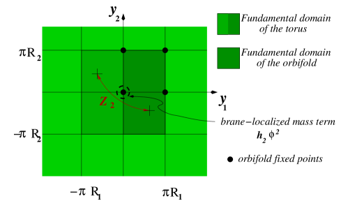
Figure 1: $\mathbb{Z}_{2}$ orbifold with a brane localized mass term for the scalar field at the origin.

2.1 The KK approach

If the scalar field $\Phi$ is even under the orbifold action, it can be decomposed on a complete basis formed by the cosine functions:

$$\Phi(x,{\bf y})=\sum_{(k_{1},k_{2})\in\mathcal{I}}\langle y_{1},y_{2}|k_{1},k_{2}\rangle\,\phi_{(k_{1},k_{2})}(x)$$ (4)

with

$$\langle y_{1},y_{2}|k_{1},k_{2}\rangle=\frac{1}{\sqrt{2\pi^{2}R_{1}R_{2}}}\frac{\cos\left(\frac{k_{1}}{R_{1}}y_{1}+\frac{k_{2}}{R_{2}}y_{2}\right)}{\sqrt{2^{\delta_{k_{1}0}\,\delta_{k_{2}0}}}}\ ,$$ (5)

The indices $k_{1,2}$ belong to the set $\mathcal{I}$

$$\mathcal{I}=\left\{(0;0),(1\ldots\infty;0),(0;1\ldots\infty),(1\ldots\infty;1\ldots\infty),(1\ldots\infty;-\infty\ldots-1)\right\}\ .$$ (6)

The scalar action (1) then takes the following form after integration over the two extra dimensions

$$\mathcal{L}=\mathcal{L}_{kin}-\frac{1}{2}\sum_{(k_{1},k_{2})\in\mathcal{I}}\left(\frac{k_{1}^{2}}{R_{1}^{2}}+\frac{k_{2}^{2}}{R_{2}^{2}}\right)\phi_{(k_{1},k_{2})}^{2}-\frac{\bar{m}^{2}}{2}\left(\sum_{(k_{1},k_{2})\in\mathcal{I}}\frac{\sqrt{2}}{\sqrt{2^{\delta_{k_{1}0}\,\delta_{k_{2}0}}}}\,\phi_{(k_{1},k_{2})}\right)^{2}\ ,$$ (7)

where

$$\bar{m}^{2}\equiv\frac{h_{2}}{4\pi^{2}R_{1}R_{2}}$$ (8)

is the naive (volume suppressed) four dimensional lightest scalar mass, which is typically of the order and slightly smaller than the compactification mass scale. The mass term of the 4D action (7) is

$$\mathcal{L}_{\rm mass}=-{1\over 2}\sum_{(k_{1},k_{2}),(p_{1},p_{2})\in\mathcal{I}}\phi_{(k_{1},k_{2})}\,\mathcal{M}^{2}_{(k_{1},k_{2}),(p_{1},p_{2})}\,\phi_{(p_{1},p_{2})}$$ (9)

with the mass matrix given by

$$\mathcal{M}^{2}_{(k_{1},k_{2}),(p_{1},p_{2})}=\frac{2\bar{m}^{2}}{\sqrt{2^{\delta_{k_{1}0}}\,2^{\delta_{k_{2}0}}}}+\left(\frac{k_{1}^{2}}{R_{1}^{2}}+\frac{k_{2}^{2}}{R_{2}^{2}}\right)\delta_{k_{1},p_{1}}\delta_{k_{2},p_{2}}\ .$$ (10)

The diagonalization of this mass matrix will define the KK mass eigenstates.

2.2 Eigenvalue Analysis

Let us now try to find the eigenvalues and eigenvectors of the mass matrix (10). The characteristic equation is given by

$$\mathcal{M}^{2}\Psi_{m}=m^{2}\Psi_{m},$$ (11)

where $m^{2}$ represents the eigenvalues and $\Psi$ is the eigenvector in the basis $\left|k_{1},k_{2}\right.\rangle_{(k_{1},k_{2})\in\mathcal{I}}$ defined in the previous section ($\Psi_{(k_{1},k_{2})}=\langle k_{1},k_{2}|\Psi_{m}\rangle$ ). The matrix equation (11) is equivalent to the infinite set of explicit equations for every $(k_{1},k_{2})\in\mathcal{I}$

$$\sqrt{2}\bar{m}^{2}\Psi^{\prime}=\sqrt{2^{\delta_{k_{1}0}\,\delta_{k_{2}0}}}\left(m^{2}-\frac{k_{1}^{2}}{R_{1}^{2}}-\frac{k_{2}^{2}}{R_{2}^{2}}\right)\Psi_{(k_{1},k_{2})},$$ (12)

where we have defined

$$\Psi^{\prime}=\sqrt{2}\sum_{(k_{1},k_{2})\in\mathcal{I}}\frac{1}{\sqrt{2^{\delta_{k_{1}0}\,\delta_{k_{2}0}}}}\Psi_{(k_{1},k_{2})}\ .$$ (13)

The solution of the equations (12) is simply given by

$$\Psi_{(k_{1},k_{2})}=\frac{1}{\sqrt{2^{\delta_{k_{1}0}\,\delta_{k_{2}0}}}}\ \frac{\mathcal{N}}{m^{2}-k_{1}^{2}/R_{1}^{2}-k_{2}^{2}/R_{2}^{2}}\ ,$$ (14)

where $\mathcal{N}$ is a normalization constant independent of $(k_{1},k_{2})$. Putting this solution back in the equation (12) for $k_{1}=k_{2}=0$, we obtain the eigenvalue equation we were searching for:

$$\frac{1}{\bar{m}^{2}}=\sum_{k_{1},k_{2}=-\infty}^{\infty}\frac{1}{m^{2}-k_{1}^{2}/R_{1}^{2}-k_{2}^{2}/R_{2}^{2}}\ .$$ (15)

Note that, in this last equation, the sums have been conveniently rewritten from $k_{i}=-\infty$ to $+\infty$ (see the identity (85) of the Appendix A).

We want to find an estimate for the lightest solution, $m^{2}$, of the eigenvalue equation. We are first going to evaluate the sums in (15) by an analytic continuation procedure in the mass eigenvalue $m=i\mu$, justified by the absence of any poles in the complex $m$ plane except for the Kaluza-Klein poles. Using the definition of the theta functions given in the Appendix, we can rewrite the eigenvalue equation as :

$$\frac{1}{\bar{m}^{2}} = -\int_{{1/\Lambda^{2}}}^{\infty}dt\ e^{-\mu^{2}t}\ \theta_{3}\left(\frac{it}{\pi R_{1}^{2}}\right)\theta_{3}\left(\frac{it}{\pi R_{2}^{2}}\right)$$ (16)

$$= -\int_{R_{c}^{2}}^{\infty}dt\ e^{-\mu^{2}t}\ \theta_{3}\left(\frac{it}{\pi R_{1}^{2}}\right)\ \theta_{3}\left(\frac{it}{\pi R_{2}^{2}}\right)$$

$$-\pi R_{1}R_{2}\int_{{1/\Lambda^{2}}}^{R_{c}^{2}}\frac{dt}{t}\ e^{-\mu^{2}t}\ \theta_{3}\left(\frac{i\pi R_{1}^{2}}{t}\right)\ \theta_{3}\left(\frac{i\pi R_{2}^{2}}{t}\right)\ ,$$

where we have introduced an UV cut-off $\Lambda$ noting that the integral is log divergent. In the following equations we consider for simplicity equal radii $R_{1}=R_{2}=R_{c}$, where $R_{c}$ defines the compactification scale. We also rewrote, using properties of the $\theta_{3}$ function defined in the appendix, the last contribution in a more convenient way.

Large Radii Limit: In the large radii limit, with respect to the cutoff $\Lambda$ and by anticipating that the lightest mass eigenvalue $m<R^{-1}$ (we will discuss in section 3 the solutions corresponding to the massive KK excitations), the approximate solution of the above eq.(16) becomes

$${1\over\bar{m}^{2}}={4\pi^{2}R_{c}^{2}\over h_{2}}\simeq-\pi R_{c}^{2}\ln({\Lambda^{2}R_{c}^{2}})+{1\over m^{2}}\ .$$ (17)

The second piece of the RHS of the above equation is the one corresponding to $k_{i}=0$: it is the infrared contribution coming from the integration region $R_{c}^{2}<t<\infty$, whereas the first piece of the RHS, logarithmically divergent, is coming from the ultraviolet region of heavy states $1/\Lambda^{2}<t<R_{c}^{2}$. The first interpretation of the result is as follows. When the radii are small, we have the ordinary “volume suppressed mass” given by :

$$m^{2}_{\rm naive}={h_{2}\over 4\pi^{2}R_{c}^{2}}\ .$$ (18)

On the other hand for large radii the logarithmic contribution from the UV has a significant effect and we get the renormalised contribution

$${1\over m^{2}}=4\pi^{2}R_{c}^{2}\left({1\over h_{2}}+{1\over 4\pi}\ln({\Lambda^{2}R_{c}^{2}})\right)\ .$$ (19)

This corresponds to the lightest eigenvalue. There is also a tower of massive KK states, the corresponding masses and their running will be presented in Section 3 (see eq (41)).

Let us now move to understand the corresponding wave function. This wave function is easily obtained from the components of $\Psi_{m}$ in the $|k_{1},k_{2}\rangle_{(k_{1},k_{2})\in\mathcal{I}}$ basis:

$$\varphi_{m}({\bf y})=\langle y_{1},y_{2}|\Psi_{m}\rangle=\sum_{(k_{1},k_{2})\in\mathcal{I}}\langle y_{1},y_{2}|k_{1},k_{2}\rangle\langle k_{1},k_{2}|\Psi_{m}\rangle\ .$$ (20)

By using the eq.(14), this is evaluated to be:

$$\varphi_{m}({\bf y})=\frac{\mathcal{N}}{\sqrt{8\pi^{2}R_{1}R_{2}}}\sum_{k_{1},k_{2}=-\infty}^{\infty}\frac{\cos(k_{1}y_{1}/R_{1}+k_{2}y_{2}/R_{2})}{m^{2}-k_{1}^{2}/R_{1}^{2}-k_{2}^{2}/R_{2}^{2}}\ ,$$ (21)

where, again, we used the even properties of the cosine functions to transform the sums into sums from $k_{i}=-\infty$ to $+\infty$.

The same results can actually be obtained in a simpler way through appropriate boundary conditions, with special care in the fixed point where the localized mass lives.

2.3 Understanding through Boundary Conditions

As in 5D where we can reformulate orbifold projections in the presence of boundary operators in terms of boundary conditions for fields propagating in the fundamental domain [23], we would like here to show that we can derive the eigenvalue equation by imposing suitable boundary conditions in 6D.

In absence of any operator localized on the fixed points, the $\mathbb{Z}_{2}$ parity assignment for an even scalar field translates into the BCs at the fixed points

$$\partial_{1}\Phi\ =\ \partial_{2}\Phi\ =\ 0\ .\$$ (22)

In the presence of the localized coupling $h_{2}$, the corresponding BCs can be read from the full equation of motion (2), which, upon the KK decomposition $\Phi(x,{\bf y})=\varphi_{m}({\bf y})\ \phi_{m}(x)$, $m$ being the 4D KK mass $\partial_{\mu}\partial^{\mu}\phi_{m}(x)+m^{2}\phi_{m}(x)=0$, reads

$$(\partial_{1}^{2}+\partial_{2}^{2}\ +\ m^{2})\ \varphi_{m}({\bf y})\ =\ h_{2}\ \varphi_{m}({\bf y})\ \delta^{2}({\bf y})\ .$$ (23)

To obtain the corresponding BCs at the origin, we first regularize the mass distribution by distributing it along a circle of radius $\epsilon$ around the origin. The mass density is related to the localized dimensionless parameter $h_{2}$ by

$$h_{2}=2\pi\,\epsilon\,m_{\epsilon}^{2}\ .$$ (24)

With this linear mass distribution, the BCs along the surface $y_{1}^{2}+y_{2}^{2}=\epsilon^{2}$ ($n$ is the normal to the surface) becomes

$$\partial_{n}\varphi=\frac{1}{2}\,m_{\epsilon}^{2}\,\varphi\$$ (25)

and when $\epsilon$ shrinks to zero, we obtain the new BCs at the origin

$$\partial_{y_{1}}\varphi=\frac{1}{2}\,h_{2}\ \varphi\,\delta(y_{2})\ ,$$

$$\partial_{y_{2}}\varphi=\frac{1}{2}\,h_{2}\ \varphi\,\delta(y_{1})\ .$$ (26)

We will now check that these BCs lead to the eigenvalue equation (15) derived earlier by the diagonalization of an infinite mass matrix. First, we note that the most general solution of the equation of motion (23) in the bulk takes the form

$$\varphi_{m}({\bf y})=\mathcal{N^{\prime}}\sum_{k_{1},k_{2}=-\infty}^{\infty}\frac{\cos(k_{1}y_{1}/R_{1}+k_{2}y_{2}/R_{2}+\alpha_{\bf k})}{m^{2}-k_{1}^{2}/R_{1}^{2}-k_{2}^{2}/R_{2}^{2}}$$ (27)

which verifies

$$(\partial_{1}^{2}+\partial_{2}^{2})\varphi_{m}=-m^{2}\varphi_{m}+\mathcal{N^{\prime}}\sum_{k_{1},k_{2}=-\infty}^{\infty}\cos(k_{1}y_{1}/R_{1}+k_{2}y_{2}/R_{2}+\alpha_{\bf k})\ .$$ (28)

In (27), $\alpha_{\bf k}$ are phases related to the position of the localised mass term. For a mass term localised at the origin, boundary conditions fix $\alpha_{\bf k}=0$. Then, by using the identity $\sum_{k=-\infty}^{\infty}\cos(ky/R)=2\pi R\ \delta(y)$, we finally obtain

$$(\partial_{1}^{2}+\partial_{2}^{2})\varphi_{m}=-m^{2}\varphi_{m}+4\pi^{2}R_{1}R_{2}\ \mathcal{N^{\prime}}\ \delta^{2}({\bf y})\ \ .$$ (29)

The comparison of the boundary terms in (23) and (29) leads to the desired eigenvalue equation (15). If the mass distribution is regularised according to (25), then the sum over the KK integers $(k_{1},k_{2})$ in (15) is effectively cut for large momenta $|k_{i}|<k_{i,max}=R_{i}/\epsilon$. The size $\epsilon$ is related to the UV cutoff defined in the previous section by $\Lambda=1/\epsilon$.

Alternatively, one can also derive the same eigenvalue equation by simply enforcing the modified BCs (2.3). To this end, one needs to massage the expression of the wavefunction (21). Actually, one of the sum can be performed by using the formula:

$$\sum_{k=-\infty}^{\infty}{\cos(kx)\over k^{2}+\alpha^{2}}={\pi\over\alpha}{\cosh\alpha(\pi-x)\over\sinh\alpha\pi}\ .$$ (30)

We obtain:

$$\varphi(y_{1},y_{2}) = -\mathcal{N^{\prime}}\pi R_{1}R_{2}\sum_{k_{2}=-\infty}^{\infty}\frac{e^{ik_{2}y_{2}/R_{2}}}{\sqrt{k_{2}^{2}-m^{2}R_{2}^{2}}}\frac{\cosh\left((R_{1}/R_{2})\sqrt{k_{2}^{2}-m^{2}R_{2}^{2}}\ (\pi-y_{1}/R_{1})\right)}{\sinh\left((\pi R_{1}/R_{2})\sqrt{k_{2}^{2}-m^{2}R_{2}^{2}}\right)}\ ,$$ (31)

which leads to the expression:

$$\partial_{y_{1}}\varphi(y_{1}=0,y_{2})=2\pi^{2}R_{1}R_{2}\ \mathcal{N^{\prime}}\ \delta(y_{2})\ .$$ (32)

Inserting this relation into the BCs at the origin, we are left again with the eigenvalue equation (15). The boundary condition in the second direction is satisfied in the same way.

3 Regularization Dependence and running

The interpretation of the logarithmic divergence in the sum is actually rather clean, by realizing that the brane localized couplings, following [19], do run in the sense of the four-dimensional renormalisation group. Our example is similar in spirit to the one analysed in [20]. It was shown there that the (euclidean) Dyson resummation of the scalar propagator, by including the brane localized mass insertions, in a mixed representation : 4d spacetime momentum space and 2d extra-dimensional coordinate space, is

$$G(q_{4},{\bf x},{\bf y}) = D(q_{4},{\bf x},{\bf y})-h_{2}\ D(q_{4},{\bf x},{\bf 0})D(q_{4},{\bf 0},{\bf y})$$ (33)

$$\ \ +h_{2}^{2}\ D(q_{4},{\bf x},{\bf 0})\ D(q_{4},{\bf 0},{\bf 0})D(q_{4},{\bf 0},{\bf y})+\cdots\$$

$$= D(q_{4},{\bf x},{\bf y})-{h_{2}\over 1+h_{2}D(q_{4},{\bf 0},{\bf 0})}\ D(q_{4},{\bf x},{\bf 0})D(q_{4},{\bf 0},{\bf y})\ ,\$$

where $D(q_{4},{\bf x},{\bf y})$ is the free scalar six-dimensional propagator of four-momentum $q_{4}$ and two-dimensional positions ${\bf x},{\bf y}$. The propagator at the origin at the compact space sum in the compact space $D(q_{4},{\bf 0},{\bf 0})$ is defined via

$$D(q_{4},{\bf 0},{\bf 0})\ =\ \sum_{\bf k}D(q_{4},{\bf k})\ \equiv\ {1\over 4\pi^{2}R_{1}R_{2}}\sum_{k_{1},k_{2}}{1\over q_{4}^{2}+k_{1}^{2}/R_{1}^{2}+k_{2}^{2}/R_{2}^{2}}\ ,\$$ (34)

where ${\bf k}=(k_{1},k_{2})$ are the Kaluza-Klein momenta in the transverse space. The pole of the resummed propagator (33) defines the physical four-dimensional masses $q_{4}^{2}=m^{2}$. One therefore gets, by going back in the Minkowski space

$${4\pi^{2}R_{1}R_{2}\over h_{2}}=\sum_{k_{1},k_{2}=-\infty}^{\infty}{1\over m^{2}-k_{1}^{2}/R_{1}^{2}-k_{2}^{2}/R_{2}^{2}}\ ,$$ (35)

which is nothing that the eigenvalue equation we derived earlier. The off-shell expression (33), however, is more suitable for renormalisation purposes since by standard techniques it leads, for $\mu>1/R_{c}$ (in the case of equal radii, $R_{1}=R_{2}=R_{c}$, that we are considering here), to the renormalisation group flow of the $h_{2}$ coupling

$$\mu{dh_{2}\over d\mu}={h_{2}^{2}\over 2\pi}\ .$$ (36)

Indeed, an approximate evaluation of the propagator for different values of the four-dimensional momentum gives

$$\sum_{\bf k}D(q_{4},{\bf k})\sim{1\over 4\pi}\ln{\Lambda^{2}\over q_{4}^{2}}\quad,\quad{\rm for}\ \ q_{4}^{2}>1/R_{c}^{2}\ ,$$

$$\sum_{\bf k}D(q_{4},{\bf k})\sim{1\over 4\pi}\ln(\Lambda^{2}R_{c}^{2})+{1\over 4\pi^{2}R_{c}^{2}q_{4}^{2}}\quad,\quad{\rm for}\ \ q_{4}^{2}<1/R_{c}^{2}\ ,$$ (37)

and therefore for $q_{4}^{2}>1/R_{c}^{2}$ the propagator exhibits a logarithmic scale dependence typical of a renormalisation group running of the coupling $h_{2}$. The coupling $h_{2}$ in the eigenvalue equation (35) is interpreted as the value of the coupling at a high cutoff scale $\Lambda$, naturally of the order of the mass scale (higher-dimensional Planck mass or the string scale) of the microscopic theory. Following this interpretation, the eigenvalue equation (35), solved under the physically relevant, for our case, situation $m\ll 1/R_{i}$ (we assume $R_{1}\sim R_{2}$ for simplicity), defines the pole mass. For energy scales $\mu>1/R_{1,2}$, the $q_{4}^{2}$ dependence can be renormalised away by an appropriate counter-term, which gives rise to the running of the mass eigenvalue:

$${1\over m^{2}(\mu)}={4\pi^{2}R_{1}R_{2}}\left({1\over h_{2}}+{1\over 2\pi}\ln{\Lambda\over\mu}\right)\equiv{4\pi^{2}R_{1}R_{2}\over h_{2}(\mu)}\ .$$ (38)

The eigenvalue equation (35) has other solutions corresponding to the massive Kaluza–Klein states. They can be easily computed in the leading approximation in $h_{2}\ll 1$ by searching solutions of the form

$$m^{2}_{(l_{1},l_{2})}=\left(\frac{l_{1}^{2}}{R_{1}^{2}}+\frac{l_{2}^{2}}{R_{2}^{2}}\right)(1+\epsilon_{l_{1},l_{2}})\quad,\quad\epsilon_{l_{1},l_{2}}\ll 1\ .$$ (39)

A straightforward computation gives

$$m^{2}_{(l_{1},l_{2})}\simeq\frac{l_{1}^{2}}{R_{1}^{2}}+\frac{l_{2}^{2}}{R_{2}^{2}}+\frac{c_{l_{1},l_{2}}}{4\pi^{2}R_{1}R_{2}}\ \left(\frac{1}{h_{2}}+\frac{1}{4\pi}\ln\frac{\Lambda^{2}}{l_{1}^{2}/R_{1}^{2}+l_{2}/R_{2}^{2}}\right)^{-1}\ .$$ (40)

$c_{l_{1},l_{2}}$ is a degeneracy factor counting the number of solutions to the integer equation $l_{1}^{2}/R_{1}^{2}+l_{2}^{2}/R_{2}^{2}=k_{1}^{2}/R_{1}^{2}+k_{2}^{2}/R_{2}^{2}$, with $k_{1},k_{2}=-\infty\ldots+\infty$. For instance, in the case of equal radii, $c_{1,1}=4$ but $c_{0,10}=12$.

Similarly to the lightest eigenvalue, the KK masses also run, but in this case the running occurs above their pole mass $\mu^{2}>m^{2}_{(l_{1},l_{2})}$

$$m_{(l_{1},l_{2})}^{2}(\mu)\simeq\frac{l_{1}^{2}}{R_{1}^{2}}+\frac{l_{2}^{2}}{R_{2}^{2}}\ +\ c_{l_{1},l_{2}}\,\frac{h_{2}(\mu)}{4\pi^{2}R_{1}R_{2}}\ .$$ (41)

4 The Fermionic Case

Before deriving the mass formula, let us first describe our framework in more detail. We will assume that the Standard Model fermions are restricted to the 4D brane whereas a singlet 6D Weyl neutrino is free to propagate in the full six dimensional space. The generalization to more than one singlet neutrino, needed in the three generation case, is straightforward. The six dimensional bulk action is simply

$$S\ =\ \int d^{4}xd^{2}y\ i\bar{\Psi}\Gamma^{M}\mathcal{D}_{M}\Psi\ .$$ (42)

Notice that no Dirac nor Majorana bulk mass is allowed for a 6D Weyl fermion.

The $\mathbb{Z}_{2}$ orbifold projection acts on $\Psi$ as

$$\mathbb{Z}_{2}\ \Psi({\bf y})\ =\ i\ e^{-(\pi/2)\,\Gamma^{5}\Gamma^{6}}\,\Psi(-{\bf y})\ .$$ (43)

Decomposing the eight-component 6D Weyl spinors into two four-component 4D Weyl spinors (see Appendix B), the $\mathbb{Z}_{2}$ action becomes

$$\Psi=\left(\begin{array}[]{c}\lambda_{1}\\ \lambda_{2}\end{array}\right),\ \ \ \ \mathbb{Z}_{2}\lambda_{1}({\bf y})=\lambda_{1}(-{\bf y}),\,\mathbb{Z}_{2}\lambda_{2}({\bf y})=-\lambda_{2}(-{\bf y})\ .$$ (44)

This allows us to write a brane localized coupling between the SM left-handed neutrino and the even fermion $\lambda_{1}$:

$$\int d^{4}x\ \ \left(h\,{\bar{\nu}}_{L}\lambda_{1}({\bf y}=0)\,H+h.c.\right)\ ,$$ (45)

where $H$ is the 4D Higgs field and $h$ is the Yukawa coupling. The mass dimensions of $\Psi,\nu_{L},H$ are respectively $5/2,3/2$ and $1$.

Written in two-component spinor notations, the 6D lagrangian takes the form :

$$\mathcal{L} = -i\lambda_{1}~{}\sigma^{\mu}~{}\partial_{\mu}\bar{\lambda}_{1}-i\lambda_{2}~{}\sigma^{\mu}~{}\partial_{\mu}\bar{\lambda}_{2}+\lambda_{1}\left(\partial_{5}+i\partial_{6}\right)\lambda_{2}$$ (46)

$$-\bar{\lambda}_{2}\left(\partial_{5}-i\partial_{6}\right)\bar{\lambda}_{1}+g_{2}(\nu_{L}\lambda_{1}+\bar{\nu}_{L}\bar{\lambda}_{1})\delta^{2}({\bf y})\ ,$$

where we have now introduced

$$g_{2}=h\langle H\rangle$$ (47)

the brane-localized ‘Dirac’ neutrino mass parameter which actually, in analogy with the scalar case, is a dimensionless parameter. We will study the phenomenology for two cases: (a) Dirac type neutrinos; (b) Majorana type neutrinos. Before proceeding further, we would like to point out that the equations of the motion are given by :

$$i\sigma^{\mu}\partial_{\mu}\bar{\lambda}_{1}-(\partial_{5}+i\partial_{6})\ \lambda_{2}=-g_{2}\ \nu_{L}\delta^{2}({\bf y})\ ,$$

$$i\sigma^{\mu}\partial_{\mu}\bar{\lambda_{2}}+(\partial_{5}+i\partial_{6})\ \lambda_{1}=0\ ,$$

$$i\sigma^{\mu}\partial_{\mu}\bar{\nu_{L}}=-g_{2}\ \lambda_{1}({\bf y}=0)\ .$$ (48)

Using the identity on the Pauli matrices given in the Appendix B, one can easily combine these coupled first order differential equations to obtain an uncoupled second order differential equation that is nothing but the Klein–Gordon equation in 6D:

$$\left(\partial_{\mu}\partial^{\mu}-\partial_{5}^{2}-\partial_{6}^{2}\right)\,\lambda_{1}(x,{\bf y})+g_{2}^{2}\ \lambda_{1}(x,{\bf y})\ \delta^{2}({\bf y})=0\$$ (49)

and therefore our fermionic problem with brane localized Dirac mass term is reduced to the one of the bulk scalar field with brane localized mass term studied in the previous Sections.

4.1 Dirac Neutrinos

Let us now study the mass matrix for the case of Dirac neutrinos. To this end we will follow the procedure first developed in the scalar case and we will expand the 6D fermion $\Psi$ on a complete set of functions. We first write the 6D Weyl fermion in terms of a pair of two-component spinors, $\lambda_{1,2}$. According to their $\mathbb{Z}_{2}$ parities, $\lambda_{1,2}$ can be decomposed as:

$$\displaystyle\lambda_{1}(x,{\bf y})=\frac{1}{\sqrt{2\pi^{2}R_{1}R_{2}}}\sum_{(k_{1},k_{2})\in\mathcal{I}}\frac{\cos(k_{1}y_{1}/R_{1}+k_{2}y_{2}/R_{2})}{\sqrt{2^{\delta_{k_{1}0}\,\delta_{k_{2}0}}}}\ \chi_{(k_{1},k_{2})}(x)\ ,$$ (50)

$$\displaystyle\lambda_{2}(x,{\bf y})=\frac{1}{\sqrt{2\pi^{2}R_{1}R_{2}}}\sum_{(k_{1},k_{2})\in\mathcal{I}}\sin(k_{1}y_{1}/R_{1}+k_{2}y_{2}/R_{2})\ \xi_{(k_{1},k_{2})}(x)\ .$$ (51)

After integration over the two extra dimensions, the mass terms in the action become

$$\mathcal{L}_{\rm mass}=\sum_{(k_{1},k_{2})\in\mathcal{I}}\left(\frac{k_{1}}{R_{1}}+i\frac{k_{2}}{R_{2}}\right)\chi_{(k_{1},k_{2})}\xi_{(k_{1},k_{2})}+\bar{m}\sum_{(k_{1},k_{2})\in\mathcal{I}}\frac{\sqrt{2}}{\sqrt{2^{\delta_{k_{1}0}\,\delta_{k_{2}0}}}}\nu_{L}\chi_{(k_{1},k_{2})}\ +h.c.$$ (52)

with

$$\bar{m}=\frac{g_{2}}{\sqrt{4\pi^{2}R_{1}R_{2}}}\ .$$ (53)

We first notice that the phases in the KK masses can be absorbed by redefining the fields $\xi_{(k_{1},k_{2})}$, while the phase in $\bar{m}$ can be removed by a redefinition of $\nu_{L}$. Thus, these phases do not have any physical effects and all the mass terms can be taken real. Next it is convenient to introduce the combinations (by convention, we define $A_{(0,0)}=\chi_{(0,0)}$ and $B_{(0,0)}=0$)

$$A_{(k_{1},k_{2})}=\frac{\chi_{(k_{1},k_{2})}+\xi_{(k_{1},k_{2})}}{\sqrt{2}}\ \ {\rm{and}}\ \ B_{(k_{1},k_{2})}=\frac{\chi_{(k_{1},k_{2})}-\xi_{(k_{1},k_{2})}}{\sqrt{2}}\ .$$ (54)

The mass terms now write

$$\frac{1}{2}\left(\nu_{L}\,A_{(k_{1},k_{2})}B_{(k_{1},k_{2})}\right)\mathcal{M}\left(\begin{array}[]{c}\nu_{L}\\ A_{(p_{1},p_{2})}\\ B_{(p_{1},p_{2})}\end{array}\right)$$ (55)

with

$$\mathcal{M}=\left(\begin{array}[]{ccc}0&\bar{m}&\bar{m}\\ \bar{m}&\vrule height=20.0pt,depth=5.0pt,width=0.0pt\sqrt{\frac{k_{1}^{2}}{R_{1}^{2}}+\frac{k_{2}^{2}}{R_{2}^{2}}}\delta_{k_{1}p_{1}}\delta_{k_{2}p_{2}}&0\\ \bar{m}&0&-\sqrt{\frac{k_{1}^{2}}{R_{1}^{2}}+\frac{k_{2}^{2}}{R_{2}^{2}}}\delta_{k_{1}p_{1}}\delta_{k_{2}p_{2}}\end{array}\right)\ .$$ (56)

The mass matrix $\mathcal{M}$ is real and symmetric. We will diagonalize is in a similar manner as we did for the scalar mass squared matrix. The characteristic equation defining the eigenvector $\Xi_{m}$ associated with the eigenvalue $m$ is

$$\mathcal{M}\ \Xi_{m}\ =\ m\ \Xi_{m}\ .$$ (57)

This matrix equation is equivalent to the infinite set of equations

$$\displaystyle\bar{m}\sum_{\mathcal{I}}\left(\langle A_{(k_{1},k_{2})}|\Xi_{m}\rangle+\langle B_{(k_{1},k_{2})}|\Xi_{m}\rangle\right)=m\langle\nu_{L}|\Xi_{m}\rangle\ ,$$ (58)

$$\displaystyle\bar{m}\langle\nu_{L}|\Xi_{m}\rangle+\sqrt{\frac{k_{1}^{2}}{R_{1}^{2}}+\frac{k_{2}^{2}}{R_{2}^{2}}}\langle A_{(k_{1},k_{2})}|\Xi_{m}\rangle=m\langle A_{(k_{1},k_{2})}|\Xi_{m}\rangle\ ,$$ (59)

$$\displaystyle\bar{m}\langle\nu_{L}|\Xi_{m}\rangle-\sqrt{\frac{k_{1}^{2}}{R_{1}^{2}}+\frac{k_{2}^{2}}{R_{2}^{2}}}\langle B_{(k_{1},k_{2})}|\Xi_{m}\rangle=m\langle B_{(k_{1},k_{2})}|\Xi_{m}\rangle\ .$$ (60)

Plugging back in eq. (58) the expressions for $\langle A_{(k_{1},k_{2})}|\Xi_{m}\rangle$ and $\langle B_{(k_{1},k_{2})}|\Xi_{m}\rangle$ obtained from eqs. (59–60), we finally obtain the desired eigenvalue equation

$$\frac{1}{\bar{m}^{2}}\ =\sum_{k_{1},k_{2}=-\infty}^{\infty}\frac{1}{m^{2}-k_{1}^{2}/R_{1}^{2}-k_{2}^{2}/R_{2}^{2}}\ .$$ (61)

4.2 Majorana Case

We now discuss the case of Majorana neutrinos. To the lagrangian discussed above (46) we want to add lepton number violating Majorana mass terms involving the Kaluza–Klein states of the bulk fermion $\Psi$. Note that there are two ways to break the lepton number : (a) Breaking the lepton number on the brane by introducing on the brane a lepton number violating mass term for the singlet neutrino; (b) Breaking the lepton number in the bulk through a bulk Majorana mass for the singlet neutrino. We will directly present the mass spectrum of these two cases in the following. Let us first study the case (a) and let us add the lepton number violating mass term $M_{0}$ on the brane

$$\int d^{4}x\ d^{2}y\ (M_{0}\ \lambda_{1}\lambda_{1}+h.c)\ \delta^{2}({\bf y})\ .$$ (62)

Notice that actually from a 6D perspective $M_{0}$ has mass dimension $-1$, whereas after the KK expansion the physical mass parameter is $M_{0}/(4\pi^{2}R_{1}R_{2})$. Similar to the Dirac mass considered previously, all phases in the Kaluza–Klein complex masses can be redefined away and have no physical meaning. By a straightforward generalisation of the previous diagonalisation, we find the eigenvalue equation

$$\frac{1}{\bar{m}^{2}+mM_{0}/(4\pi^{2}R_{1}R_{2})}\ =\sum_{k_{1},k_{2}=-\infty}^{\infty}\frac{1}{m^{2}-k_{1}^{2}/R_{1}^{2}-k_{2}^{2}/R_{2}^{2}}\ .$$ (63)

By considering again for simplicity the case of two equal radii $R_{1}=R_{2}=R_{c}$ and evaluating as before the double sum by keeping the leading IR and UV contributions, we find in the large radii limit

$$\frac{1}{m^{2}}=4\pi^{2}R_{c}^{2}\left(\frac{1}{g_{2}^{2}+mM_{0}}+\frac{1}{4\pi}\ln(\Lambda^{2}R_{c}^{2})\right)\ .$$ (64)

The natural interpretation is again in terms of the running of the physical mass

$$\frac{1}{m^{2}(\mu)}\ =\ \frac{4\pi^{2}R_{c}^{2}}{(g_{2}^{2}+mM_{0})(\mu)}\ .$$ (65)

The case of the brane Majorana mass is the simplest but also the most problematic, since due to the double volume suppression the lepton number violation, is small. The case of the bulk Majorana mass $M$ is more subtle. First of all, a standard Majorana, Lorentz invariant mass in 6D, ${\bar{\Psi}}^{C}\Psi$ cannot be written for a Weyl fermion, since it mixes 6D Weyl fermions of opposite chiralities. On the other hand, a Majorana mass term involving only a 6D Weyl fermion, of the form ${\bar{\Psi}}^{C}\Gamma_{6}\Psi$ can be written, at the expense of breaking the 6D Lorentz symmetry which could be considered as being spontaneously generated by the vev of some vector field. In this case, it is not possible anymore to eliminate the phases in the KK masses by field redefinitions, even for real Majorana mass. Interestingly enough, the interplay between Kaluza–Klein masses and bulk Lorentz violating Majorana mass generates CP violation. This observation could be related to previous proposals to relate the CP symmetry to discrete subgroups of a higher-dimensional Lorentz group [24]. The eigenvalue equation in this case is

$$\frac{g_{2}^{2}}{4\pi^{2}R_{1}R_{2}}\ \sum_{k_{1},k_{2}=-\infty}^{\infty}\frac{1}{m-M-ik_{1}/R_{1}+k_{2}/R_{2}}\ =\ m\ .$$ (66)

5 Neutrino oscillations

Generally, the gauge neutrino eigenstates $\nu_{f}$ are related to the set of mass eigenstates ${\tilde{\nu}}_{i}$ through a unitary mixing matrix $U$ as

$$\nu_{f}=\sum_{i}U_{fi}{\tilde{\nu}}_{i}\ ,$$ (67)

where the matrix $U$ is extracted from the neutrino mass matrix. The probability of oscillation between two gauge eigenstates $\nu_{f}$ and $\nu_{f}^{\prime}$ after a time $t$ is given by

$$P_{f\rightarrow f^{\prime}}(t)=\sum_{i}\left|U_{fi}U_{f^{\prime}i}\right|^{2}+2\sum_{i>j}{\rm Re}\left(U_{fi}U^{*}_{f^{\prime}i}U^{*}_{fj}U_{f^{\prime}j}e^{[i(E_{j}-E_{i})t]}\right)\ ,$$ (68)

where $E_{i}=\sqrt{p^{2}+m_{i}^{2}}$ is the energy of the mass eigenstate ${\tilde{\nu}}_{i}$. Of a particular interest for our case where the active neutrinos oscillates into bulk states is the survival probability after a time $t$, given by

$$P_{f\rightarrow f}(t)=\left|\ \sum_{i}|U_{fi}|^{2}e^{iE_{i}t}\ \right|^{2}\ .$$ (69)

We consider in the following the case of the Dirac neutrinos discussed in detail in Section 4. The matrix $U$ in this case is (doubly) infinite dimensional and, from (58)-(60) its explicit form is

$$\displaystyle\langle\Xi_{m_{i}}|U|\nu_{L}\rangle=\frac{1}{\sqrt{N_{i}}}\ ,$$ (70)

$$\displaystyle\langle\Xi_{m_{i}}|U|A_{(k_{1},k_{2})}\rangle=\frac{1}{\sqrt{N_{i}}}\,\frac{\bar{m}}{m_{i}-\sqrt{k_{1}^{2}/R_{1}^{2}+k_{2}^{2}/R_{2}^{2}}}\ ,\ (k_{1},k_{2})\in\mathcal{I}\ ,$$ (71)

$$\displaystyle\langle\Xi_{m}|U|B_{(k_{1},k_{2})}\rangle=\frac{1}{\sqrt{N_{i}}}\,\frac{\bar{m}}{m_{i}+\sqrt{k_{1}^{2}/R_{1}^{2}+k_{2}^{2}/R_{2}^{2}}}\ ,\ (k_{1},k_{2})\in\mathcal{I}\backslash(0,0)\ .$$ (72)

The unitarity property of the $U$ matrix determines the normalisation constant, $N_{i}$, to be

$$N_{i} = 1+\bar{m}^{2}\sum_{k_{1},k_{2}=-\infty}^{\infty}\frac{m_{i}^{2}+k_{1}^{2}/R_{1}^{2}+k_{2}^{2}/R_{2}^{2}}{\left(m_{i}^{2}-k_{1}^{2}/R_{1}^{2}-k_{2}^{2}/R_{2}^{2}\right)^{2}}$$ (73)

$$= 2\bar{m}^{2}m_{i}^{2}\sum_{k_{1},k_{2}=-\infty}^{\infty}\frac{1}{\left(m_{i}^{2}-k_{1}^{2}/R_{1}^{2}-k_{2}^{2}/R_{2}^{2}\right)^{2}}$$

where the eigenvalue equation (15) has been used to arrive at the last expression. We notice that the last summation (73) is manifestly UV finite and therefore the only cutoff dependence arise implicitly through the running of the physical neutrino masses. The active neutrino survival probability, in the non-relativistic approximation, is then given by the formula [9]

$$P_{\nu_{L}\rightarrow\nu_{L}}(t)=\left|\sum_{(k_{1},k_{2})\in\mathcal{I}}\frac{2}{N_{(k_{1},k_{2})}}\ e^{i\frac{m_{(k_{1},k_{2})}^{2}t}{2p}}\ \right|^{2}=\left|\sum_{k_{1},k_{2}=-\infty}^{\infty}\frac{2^{\delta_{k_{1}0}\delta_{k_{2}0}}}{N_{(k_{1},k_{2})}}\ e^{i\frac{m_{(k_{1},k_{2})}^{2}t}{2p}}\ \right|^{2}\ .$$ (74)

The factor 2 in the first sum accounts for the fact that each massive state corresponds to a Dirac neutrino. An approximate estimation of the normalisation factors $N_{(k_{1},k_{2})}$ gives the result

$$N_{(k_{1},k_{2})}\ \simeq\ c_{k_{1},k_{2}}\ \frac{2\bar{m}^{2}m_{(k_{1},k_{2})}^{2}}{\left(m_{(k_{1},k_{2})}^{2}-k_{1}^{2}/R_{1}^{2}-k_{2}^{2}/R_{2}^{2}\right)^{2}}$$ (75)

where $m_{(k_{1},k_{2})}$ is the pole mass eigenvalue given by the eq. (40) and $c_{k_{1},k_{2}}$ are the degeneracy factors defined in Section 3. We can anticipate from (75) some similarities and also some differences between the 5D and the present 6D case. Like in the 5D case [9], for large KK masses $N_{i}\sim m_{i}^{2}$ and the active neutrino mostly oscillates into the lowest mass states. In the 6D case, on the other hand, the degeneracy of the massive states is higher than in 5D and the decoupling of the massive states is slower than in 5D.

Numerically too, we find similar behaviour. For a relatively small number of states, $P(t)$ is always smaller than $1$. In fact, even $P(0)$ is smaller than 1, unless one sums over all the states. $P(t)$ oscillates with $t$, though it is always remaining smaller than $P(0)$. The oscillations become more rapid as we sum over more and more states.

The brane Majorana case can simply be recovered from the previous expressions by the replacement ${\bar{m}}^{2}\rightarrow{\bar{m}}^{2}+m_{i}M_{0}$.

6 Phenomenology

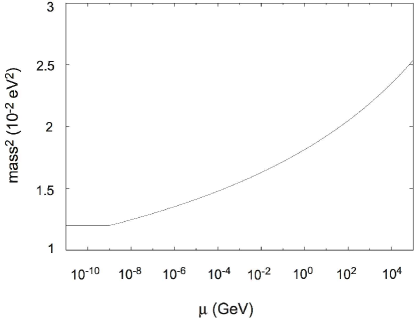
Figure 2: Running of the neutrino squared masses with the energy. We have chosen $\Lambda~{}=~{}10^{5}$ GeV, $g_{2}~{}=~{}1$, and $R_{1}~{}=~{}R_{2}~{}=~{}1$ eV^-1. The running occurs between the cutoff scale and the compactification scale. Below the compactification scale, there is not running anymore.

In this Section, we will detail some phenomenological consequences which could be of interest for neutrino masses and mixings. First of all, let us try to see the significance of the logarithmic running with some realistic numbers. Fig. 2 plots the running of the neutrino mass-squared with the energy. We have taken the radii to be of the order of 1 eV^-1 with the fundamental Planck scale $M_{\star}$ taken to be around 100 TeV, in order to recover the 4D Planck scale $M_{P}$ through the standard relation $R_{1}R_{2}M_{\star}^{4}=M_{P}^{2}$ [1]. Note that these numbers are close to the present limits from cosmology on the size of two large extra dimensions [26]. The coupling $g_{2}$ is set to one at the cutoff (microscopic) scale. We plot eq. (38) and we see that the neutrino mass changes by at least a factor of $3$ while running with the radius. Below $R^{-1}$, there is no logarithmic running anymore and the masses keep their values at the compactification scale. This explains the horizontal line below $R^{-1}$. We interpret this result as follows. The pole of the propagator as given in eq. (35), defines the physical mass of the neutrino which is equivalent to the ‘running’ eigenvalue evaluated at $R^{-1}$. As long as neutrinos are ‘on-shell’, they carry this mass. The ‘running’ neutrino masses on the other hand varies with the off-shell momentum. Experimentally, the effect of this ‘running’ could be possibly seen in processes where neutrinos are off-shell. The best probed process in this regard is neutrinoless double beta decay which involves lepton number violating neutrino masses. We note only that as long as the lepton number is violated by Majorana masses and the running of the Dirac masses does occur, this is enough to have observable effects due to the running between the pole mass and the off-shell momentum, of the order the nucleon mass, in the neutrinoless double beta decay diagrams. A detailed analysis of this case is beyond our goal here. On the other hand, irrespective of whether lepton number is violated or not, this running should always be considered while constructing models of fermion masses in 6D. This is especially true in models where large radii are considered. One can interpret that the ‘bare’ couplings in the lagrangian given at the scale $\Lambda$ would get modified as they ‘run’ towards their physical values. While most of the present discussion has been concentrated for the case of a single generation, we can easily extend the above analysis for more than one flavour. First of all, it is useful to recall that in order to generate three non-vanishing masses for the three active neutrinos, we need to introduce three distinct bulk sterile Weyl fermions $\Psi_{a}$ and therefore the brane-bulk mixing mass term becomes a $3\times 3$ matrix. The obvious change in the RGE evolution of the dimensionless coupling $h_{2}\equiv g_{2}^{2}$ is

$$\mu{d(h_{2})_{ab}\over d\mu}\ =\ {1\over 2\pi}\ (h_{2})_{ac}(h_{2})_{cb}\ ,$$ (76)

whereas the $3\times 3$ lightest eigenvalue mass matrix has the RGE evolution

$$\biggl{(}{1\over m^{2}(\mu)}\biggr{)}_{ab}\ =\ {4\pi^{2}R_{1}R_{2}}\left[\biggl{(}{1\over h_{2}}\biggr{)}_{ab}+{1\over 2\pi}\ \delta_{ab}\ln{\Lambda\over\mu}\right]\equiv{4\pi^{2}R_{1}R_{2}}\ \biggl{(}{1\over h_{2}(\mu)}\biggr{)}_{ab}\ .$$ (77)

The classical running then modifies the flavour mixing present at the scale $\Lambda$ by renormalising it in evolving towards low energy. Since in order to have sizable running the active neutrinos are required not to be much lighter than the sterile neutrinos, the oscillations into the bulk sterile states are constrained by the existing experimental data. The two flavour active-sterile oscillations can be suppressed by choosing a sufficiently small coupling $h_{2}$. For example, for $h_{2}~{}=~{}0.05$ we find (for $\Lambda=100$ GeV and summing up to first 200 states), that the survival probability of the active neutrinos can stay around 70%. The survival probability obviously decreases as $h_{2}$ increases. When other active flavours are added, since mass differences for active neutrinos $\Delta m^{2}_{\nu_{e}\nu_{\mu}},\Delta m^{2}_{\nu_{e}\nu_{\tau}}\ll R_{c}^{-2}\sim eV^{2}$, for small values of the coupling $g_{2}$ and for all KK states the mass differences $m_{\nu_{i}}^{2}-m_{KK}^{2}\gg\Delta m^{2}_{\nu_{e}\nu_{\mu}},\Delta m^{2}_{\nu_{e}\nu_{\tau}}$. In this case, the oscillations into sterile neutrinos are subdominant with respect to active neutrino oscillations. Obviously, the above results are qualitative and a full phenomenological analysis is required. We postpone it for a later work.

It is more useful to write the running neutrino mass directly as a function of the physical pole mass $m_{\nu}^{2}$. In the case of Dirac neutrinos and for one generation, for simplicity, we get

$$m_{\nu}^{2}(\mu)\ =\ m_{\nu}^{2}\ \frac{1+{g_{2}^{2}\over 2\pi}\ln(\Lambda R_{c})}{1+{g_{2}^{2}\over 2\pi}\ln({\Lambda\over\mu})}\ .$$ (78)

This running is a small effect for small couplings $g_{2}$. For example, for radii $R_{c}^{-1}\sim{\rm eV}$ and in the normal hierarchical neutrinos scenario, the coupling $g_{2}$ for the electron neutrino has to be of order $10^{-2}$. In this case, the running (78) in the energy range eV and GeV is too small to have observable effects. In the inverse hierarchy (or almost degenerate) neutrinos scenario, however, for $g_{2}\sim\mathcal{O}(1)$, the effect is large, as already stressed. This fits well with the fact that neutrinoless double beta decay amplitude, proportional to the effective Majorana mass

$$m_{ee}\ =\ \sum_{a}U_{ea}^{2}m_{a}\ ,$$ (79)

where $a$ are the three active neutrino states, increases with the absolute value of the neutrino masses.

The question then remains about other physical effects of the sterile neutrinos. For the large radii, $R_{c}\sim\mathcal{O}({\rm eV}^{-1})-\mathcal{O}({\rm keV}^{-1})$, we should expect a large number of very light sterile states. The effects of the virtual sterile states in loop processes involving neutrinos, in astrophysics and cosmology need a separate careful analysis, which is very important for the validity of the models we proposed in this paper. This is beyond the goals of the present work. We notice here, however, that the running of the neutrino masses is valid also for smaller values of the compact radii, even if in this case the effect of the running becomes much smaller and it will be harder to detect experimentally.

Appendix A: Jacobi function

The Jacobi function $\theta_{3}$ used in the text is defined as

$$\theta_{3}(z|\tau)=\sum_{k=-\infty}^{\infty}e^{2\pi ikz+i\pi k^{2}\tau}\ .$$ (80)

A useful modular transformation property is

$$\theta_{3}\left({z\over\tau},{-1\over\tau}\right)=\sqrt{-i\tau}\ e^{{i\pi z^{2}/\tau}}\ \theta_{3}(z,\tau)\ .$$ (81)

The asymptotic limits of $\theta_{3}$ that we used are

$$\lim_{t\rightarrow\infty}\ \theta_{3}(z|\tau=it)=1\quad,\quad\lim_{t\rightarrow 0}\ \theta_{3}(z|\tau=it)\sim{1\over\sqrt{t}}\ e^{-{\pi z^{2}\over t}}\ .$$ (82)

We denote $\theta_{3}(0|\tau)$ by $\theta_{3}(\tau)$.

We can rewrite the eigenvalue equation (15) by using the Jacobi $\theta_{3}$ function. Indeed, by introducing the Schwinger proper time parameter $t$ through

$${1\over A}\ =\ \int_{0}^{\infty}dt\ e^{-tA}\ \$$ (83)

and using the analytic continuation prescription $m=i\mu$, we find

$$\sum_{k_{1},k_{2}=-\infty}^{\infty}\frac{1}{m^{2}-k_{1}^{2}/R_{1}^{2}-k_{2}^{2}/R_{2}^{2}}=-\int_{1/\Lambda^{2}}^{\infty}\ dt\ e^{-\mu^{2}t}\ \theta_{3}\left(\frac{it}{\pi R_{1}^{2}}\right)\theta_{3}\left(\frac{it}{\pi R_{2}^{2}}\right)\ .$$ (84)

Let us also mention the identity

$$\sum_{(k_{1},k_{2})\in\mathcal{I}}\frac{2}{2^{\delta_{k_{1}0}\delta_{k_{2}0}}}f(k_{1},k_{2})=\sum_{k_{1},k_{2}=-\infty}^{\infty}f(k_{1},k_{2})\ ,$$ (85)

valid for any function $f$ such that $f(-k_{1},-k_{2})=f(k_{1},k_{2})$ and where $\mathcal{I}$ is the set defined in eq.(6).

Appendix B: 6D Dirac matrices

For completeness, we give in this appendix the convention about spinors and Dirac matrices used throughout the paper. We have mainly followed the conventions of Wess and Bagger [25].

In 6D, the Dirac matrices are $8\times 8$ and they can be easily constructed from the Dirac matrices in 4D:

$$\Gamma^{\mu}=\left(\begin{array}[]{cc}\gamma^{\mu}&0\\ 0&\gamma^{\mu}\end{array}\right)_{\mu=0,1,2,3}\,,\ \Gamma^{5}=\left(\begin{array}[]{cc}0&i\gamma^{5}\\ i\gamma^{5}&0\end{array}\right)\ \ \mathrm{and}\ \ \Gamma^{6}=\left(\begin{array}[]{cc}0&-\gamma^{5}\\ \gamma^{5}&0\end{array}\right)$$ (86)

with

$$\gamma^{\mu}=\left(\begin{array}[]{cc}0&\sigma^{\mu}\\ \bar{\sigma}^{\mu}&0\end{array}\right)\ \ \mathrm{and}\ \ \gamma^{5}=i\gamma^{0}\ldots\gamma^{3}=\left(\begin{array}[]{cc}-\sigma^{0}&0\\ 0&\sigma^{0}\end{array}\right)$$ (87)

where $\sigma^{\mu}$ and $\bar{\sigma}^{\mu}$ are the usual Pauli matrices

$$\sigma^{0}=-\mathbf{1}_{2},\,\sigma^{1}=\left(\begin{array}[]{cc}0&1\\ 1&0\end{array}\right),\sigma^{2}=\left(\begin{array}[]{cc}0&-i\\ i&0\end{array}\right),\sigma^{3}=\left(\begin{array}[]{cc}1&0\\ 0&-1\end{array}\right),$$ (94)

$$\vrule height=13.0pt,depth=5.0pt,width=0.0pt\bar{\sigma}^{0}=\sigma^{0},\,\bar{\sigma}^{1}=-\sigma^{1},\,\bar{\sigma}^{2}=-\sigma^{2},\,\bar{\sigma}^{3}=-\sigma^{3}.$$ (95)

A famous relation about the Pauli matrices that is useful to link the fermionic equation of motion to the scalar equation of motion is

$$\sigma^{\mu}\bar{\sigma}^{\nu}+\sigma^{\nu}\bar{\sigma}^{\mu}=2\eta^{\mu\nu}\ \ \mathrm{and}\ \ \bar{\sigma}^{\mu}\sigma^{\nu}+\bar{\sigma}^{\nu}\sigma^{\mu}=2\eta^{\mu\nu}.$$ (96)

The chirality matrix in 6D is simply defined by

$$\Gamma^{7}=\Gamma^{0}\ldots\Gamma^{3}\Gamma^{5}\Gamma^{6}=\left(\begin{array}[]{cc}\gamma^{5}&0\\ 0&-\gamma^{5}\end{array}\right)\ .$$ (97)

Therefore a 6D Weyl fermion is written in terms of a pair of four-component Weyl fermions

$$\Psi=\left(\begin{array}[]{c}\lambda_{1}\\ \lambda_{2}\end{array}\right)\ ,$$ (98)

with

$$\Psi=-\Gamma^{7}\Psi\ \ \Leftrightarrow\ \ \lambda_{1}=-\gamma^{5}\lambda_{1},\ \lambda_{2}=\gamma^{5}\lambda_{2}\ .$$ (99)

The four-component Weyl fermions can be themselves conveniently written as two-components spinors (we’ll use the same notation for a four and two component spinor, the distinction should be clear from the context)

$$\lambda_{1}=\left(\begin{array}[]{c}0\\ \bar{\lambda}^{\dot{\alpha}}_{1}\end{array}\right)\ ,\ ~{}~{}~{}~{}\lambda_{2}=\left(\begin{array}[]{c}\lambda_{2\,\alpha}\\ 0\end{array}\right)\ .$$ (100)

The dotted and undotted indices of a two-component spinor are raised and lower with the $2\times 2$ antisymmetric tensors $\epsilon_{\alpha\beta}=i\sigma^{2}_{\alpha\beta}$ and $\epsilon_{\dot{\alpha}\dot{\beta}}=i\sigma^{2}_{\dot{\alpha}\dot{\beta}}$ and their inverse $\epsilon^{\alpha\beta}=-i\sigma^{2}_{\alpha\beta}$, $\epsilon^{\dot{\alpha}\dot{\beta}}=-i\sigma^{2}_{\dot{\alpha}\dot{\beta}}$ :

$$\lambda_{2}^{\alpha}=\epsilon^{\alpha\beta}\lambda_{2\,\beta}\ \ \mathrm{and}\ \ \bar{\lambda}_{1\,\dot{\alpha}}=\epsilon_{\dot{\alpha}\dot{\beta}}\bar{\lambda}_{1}^{\dot{\beta}}\ .$$ (101)

Note also the adjoint relation:

$$(\lambda_{2}^{\dagger})^{\alpha}=\bar{\lambda}_{2}^{\dot{\alpha}}\ .$$ (102)

Finally, $\lambda_{1}\lambda_{2}$ and $\bar{\lambda}_{1}\bar{\lambda}_{2}$ denote the two Lorentz invariant scalars:

$$\lambda_{1}\lambda_{2}=\lambda_{1}^{\alpha}\lambda_{2\,\alpha}\ \ \mathrm{and}\ \ \bar{\lambda}_{1}\bar{\lambda}_{2}=\bar{\lambda}_{1\,\dot{\alpha}}\bar{\lambda}_{2}^{\dot{\alpha}}\ .$$ (103)

These products are symmetric

$$\lambda_{1}\lambda_{2}=\lambda_{2}\lambda_{1}\ \ \mathrm{and}\ \ \bar{\lambda}_{1}\bar{\lambda}_{2}=\bar{\lambda}_{2}\bar{\lambda}_{1}\ .$$ (104)

The charge conjugation matrix in six dimensions, satisfying

$$C\ \Gamma^{M}\ C^{-1}\ =\ -(\Gamma^{M})^{T}\ ,$$ (105)

can be expressed in terms of the 4D one as

$$C\ =\ \left(\begin{array}[]{cc}0&C_{4}\\ -C_{4}&0\end{array}\right)\ ,$$ (106)

where

$$C_{4}\ \gamma^{\mu}\ C_{4}^{-1}\ =\ -(\gamma^{\mu})^{T}\ .$$ (107)

In the chiral representation of the Dirac matrices that we are using,

$$C_{4}=i\gamma^{0}\gamma^{2}=\left(\begin{array}[]{cc}i\sigma^{2}&0\\ 0&-i\sigma^{2}\end{array}\right)$$ (108)

It can be easily checked that

$$C\ \Gamma^{7}=-\Gamma^{7}\ C\ \ {\rm and}\ \ C^{\dagger}\ =\ C\ .$$ (109)

The charged conjugated spinor $\Psi^{c}$ is defined through

$$\Psi^{c}=C\bar{\Psi}^{T}\ .$$ (110)

It can be easily checked that for the 6D Weyl spinor satisfying eqs. (99), we have (in four and two component notations):

$$\displaystyle{\bar{\Psi}}\Psi\ =\ 0\ ,\ {\bar{\Psi}}^{c}\Psi\ =\ 0\ ,$$ (111)

$$\displaystyle{\bar{\Psi}}^{c}\Gamma^{5}\Psi=i\left(\lambda_{2}^{t}C_{4}\lambda_{2}+\lambda_{1}^{t}C_{4}\lambda_{1}\right)=-\left(\bar{\lambda}_{1}\bar{\lambda}_{1}+\lambda_{2}\lambda_{2}\right)\ ,$$ (112)

$$\displaystyle{\bar{\Psi}}^{c}\Gamma^{6}\Psi=-\lambda_{2}^{t}C_{4}\lambda_{2}+\lambda_{1}^{t}C_{4}\lambda_{1}=-\bar{\lambda}_{1}\bar{\lambda}_{1}+\lambda_{2}\lambda_{2}\ .$$ (113)

Acknowledgements : We are grateful to G. Bhattacharyya, T. Gherghetta, P. Holstein, S. Lavignac, J. Mourad, C. Papineau, M. Peloso, K. Sridhar and especially to V. Rubakov for suggestions and discussions. SKV acknowledges support from Indo-French Centre for Promotion of Advanced Research (CEFIPRA) project No: 2904-2 ‘Brane World Phenomenology’. We all acknowledge the hospitality of the Department of Theoretical Physics of TIFR-Mumbai, whereas E.D. would like to thanks the hospitality of the William I. Fine Theoretical Physics Institute of the University of Minnesota while completing this work. Work partially supported by INTAS grant, 03-51-6346, CNRS PICS # 2530 and 3059, RTN contracts MRTN-CT-2004-005104 and MRTN-CT-2004-503369, a European Union Excellence Grant, MEXT-CT-2003-509661 and by the ACI Jeunes Chercheurs 2068.

References

• [1] N. Arkani-Hamed, S. Dimopoulos and G. R. Dvali, Phys. Lett. B 429, 263 (1998) [arXiv:hep-ph/9803315] ; I. Antoniadis, N. Arkani-Hamed, S. Dimopoulos and G. R. Dvali, Phys. Lett. B 436, 257 (1998) [arXiv:hep-ph/9804398].
• [2] I. Antoniadis, Phys. Lett. B 246, 377 (1990).
• [3] L. Randall and R. Sundrum, Phys. Rev. Lett.  83, 3370 (1999) [arXiv:hep-ph/9905221] ; Phys. Rev. Lett.  83 (1999) 4690 [arXiv:hep-th/9906064] ; M. Gogberashvili, Int. J. Mod. Phys. D 11 (2002) 1635 [arXiv:hep-ph/9812296].
• [4] K. R. Dienes, E. Dudas and T. Gherghetta, Phys. Lett. B 436, 55 (1998) [arXiv:hep-ph/9803466]; K. R. Dienes, E. Dudas and T. Gherghetta, Nucl. Phys. B 537, 47 (1999) [arXiv:hep-ph/9806292].
• [5] A. Delgado, A. Pomarol and M. Quiros, JHEP 0001, 030 (2000) [arXiv:hep-ph/9911252]; T. Appelquist, H. C. Cheng and B. A. Dobrescu, Phys. Rev. D 64 (2001) 035002 [arXiv:hep-ph/0012100].
• [6] G. F. Giudice, R. Rattazzi and J. D. Wells, Nucl. Phys. B 544, 3 (1999) [arXiv:hep-ph/9811291]; E. A. Mirabelli, M. Perelstein and M. E. Peskin, Phys. Rev. Lett.  82 (1999) 2236 [arXiv:hep-ph/9811337]; T. Han, J. D. Lykken and R. J. Zhang, Phys. Rev. D 59 (1999) 105006 [arXiv:hep-ph/9811350].
• [7] Y. Fukuda et al. [Super-Kamiokande Collaboration], Phys. Rev. Lett.  81 (1998) 1562 [arXiv:hep-ex/9807003]; S. Fukuda et al. [Super-Kamiokande Collaboration], Phys. Rev. Lett.  86 (2001) 5651 [arXiv:hep-ex/0103032].
• [8] P. Minkowski, Phys. Lett. B 67 (1977) 421 ; M. Gell-Mann, P. Ramond and R. Slansky, in (P. van Nieuwenhuisen and D.Z. Freedman eds.), North-Holland, Amsterdam, 1979; T. Yanagida, in Proceedings of the Workshop on Unified Theories and Baryon Number in the Universe (A. Sawada and A. Sugamoto eds.), KEK preprint 79-18, 1979; R. N. Mohapatra and G. Senjanovic, Phys. Rev. Lett.  44 (1980) 912.
• [9] K. R. Dienes, E. Dudas and T. Gherghetta, Nucl. Phys. B 557, 25 (1999) [arXiv:hep-ph/9811428]; K. R. Dienes and I. Sarcevic, Phys. Lett. B 500 (2001) 133 [arXiv:hep-ph/0008144].
• [10] N. Arkani-Hamed, S. Dimopoulos, G. R. Dvali and J. March-Russell, Phys. Rev. D 65 (2002) 024032 [arXiv:hep-ph/9811448] ; G. R. Dvali and A. Y. Smirnov, Nucl. Phys. B 563 (1999) 63 [arXiv:hep-ph/9904211].
• [11] R. N. Mohapatra, S. Nandi and A. Perez-Lorenzana, Phys. Lett. B 466 (1999) 115 [arXiv:hep-ph/9907520]; A. Ioannisian and A. Pilaftsis, Phys. Rev. D 62 (2000) 066001 [arXiv:hep-ph/9907522]; R. Barbieri, P. Creminelli and A. Strumia, Nucl. Phys. B 585 (2000) 28 [arXiv:hep-ph/0002199]; A. Lukas, P. Ramond, A. Romanino and G. G. Ross, Phys. Lett. B 495 (2000) 136 [arXiv:hep-ph/0008049] and JHEP 0104 (2001) 010 [arXiv:hep-ph/0011295]; A. De Gouvea, G. F. Giudice, A. Strumia and K. Tobe, Nucl. Phys. B 623, 395 (2002) [arXiv:hep-ph/0107156]; G. Bhattacharyya, H. V. Klapdor-Kleingrothaus, H. Paes and A. Pilaftsis, Phys. Rev. D 67 (2003) 113001 [arXiv:hep-ph/0212169].
• [12] Y. Grossman and M. Neubert, Phys. Lett. B 474 (2000) 361 [arXiv:hep-ph/9912408]; T. Gherghetta and A. Pomarol, Nucl. Phys. B 586 (2000) 141 [arXiv:hep-ph/0003129].
• [13] I. Antoniadis, K. Benakli and M. Quiros, New J. Phys.  3, 20 (2001) [arXiv:hep-th/0108005]; C. Csáki, C. Grojean and H. Murayama, Phys. Rev. D 67, 085012 (2003) [arXiv:hep-ph/0210133] ; G. von Gersdorff and M. Quiros, Phys. Rev. D 68 (2003) 105002 [arXiv:hep-th/0305024].
• [14] T. Appelquist, B. A. Dobrescu, E. Ponton and H. U. Yee, Phys. Rev. Lett.  87, 181802 (2001) [arXiv:hep-ph/0107056].
• [15] B. A. Dobrescu and E. Poppitz, Phys. Rev. Lett.  87, 031801 (2001) [arXiv:hep-ph/0102010].
• [16] G. Servant and T. M. P. Tait, Nucl. Phys. B 650 (2003) 391 [arXiv:hep-ph/0206071].
• [17] T. Asaka, W. Buchmuller and L. Covi, Phys. Lett. B 523, 199 (2001) [arXiv:hep-ph/0108021] and Nucl. Phys. B 648, 231 (2003) [arXiv:hep-ph/0209144]; L. J. Hall, Y. Nomura, T. Okui and D. R. Smith, Phys. Rev. D 65 (2002) 035008 [arXiv:hep-ph/0108071].
• [18] T. Appelquist, B. A. Dobrescu, E. Ponton and H. U. Yee, Phys. Rev. D 65, 105019 (2002) [arXiv:hep-ph/0201131]; J. Matias and C. P. Burgess, arXiv:hep-ph/0508156.
• [19] H. Georgi, A. K. Grant and G. Hailu, Phys. Lett. B 506 (2001) 207 [arXiv:hep-ph/0012379].
• [20] W. D. Goldberger and M. B. Wise, Phys. Rev. D 65 (2002) 025011 [arXiv:hep-th/0104170].
• [21] C. P. Bachas, JHEP 9811 (1998) 023 [arXiv:hep-ph/9807415]; I. Antoniadis and C. Bachas, Phys. Lett. B 450 (1999) 83 [arXiv:hep-th/9812093]; I. Antoniadis, C. Bachas and E. Dudas, Nucl. Phys. B 560 (1999) 93 [arXiv:hep-th/9906039]; N. Arkani-Hamed, S. Dimopoulos and J. March-Russell, arXiv:hep-th/9908146.
• [22] B. A. Dobrescu and E. Ponton, JHEP 0403, 071 (2004) [arXiv:hep-th/0401032]; G. Burdman, B. A. Dobrescu and E. Ponton, arXiv:hep-ph/0506334.
• [23] C. Csáki, C. Grojean, H. Murayama, L. Pilo and J. Terning, Phys. Rev. D 69, 055006 (2004) [arXiv:hep-ph/0305237]; C. Csáki, C. Grojean, L. Pilo and J. Terning, Phys. Rev. Lett.  92, 101802 (2004) [arXiv:hep-ph/0308038]; Z. Chacko, M. Graesser, C. Grojean and L. Pilo, Phys. Rev. D 70, 084028 (2004) [arXiv:hep-th/0312117]; G. Cacciapaglia, C. Csáki, C. Grojean, M. Reece and J. Terning, arXiv:hep-ph/0505001.
• [24] K. w. Choi, D. B. Kaplan and A. E. Nelson, Nucl. Phys. B 391 (1993) 515 [arXiv:hep-ph/9205202].
• [25] J. Wess and J. Bagger, “Supersymmetry and supergravity,” Princeton, Univ. Press, 1992; J. A. Bagger, arXiv:hep-ph/9604232.
• [26] S. Cullen and M. Perelstein, Phys. Rev. Lett.  83, 268 (1999) [arXiv:hep-ph/9903422]; L. J. Hall and D. R. Smith, Phys. Rev. D 60, 085008 (1999) [arXiv:hep-ph/9904267].