Current and Future Limits on General Flavour Violation in $b\rightarrow s$ Transitions in Minimal Supersymmetry

Abstract:

We discuss the current and prospective limits that can be placed on supersymmetric contributions to $b\to s$ transitions in the Minimal Supersymmetric Standard Model with general flavour mixing amongst the squarks. We consider three processes: $\bar{B}\to X_{s}\gamma$, $\bar{B}_{s}\to\mu^{+}\mu^{-}$ and $\bar{B}_{s}-B_{s}$ mixing, and pay particular attention to the large $\tan\beta$ regime and beyond leading order contributions where the difference between our analysis and previous analyses is most pronounced. We find that even present limits on $\mathrm{BR}(\bar{B}_{s}\to\mu^{+}\mu^{-})$ and $\Delta M_{B_{s}}$ often provide additional constraints on the amount of flavour violation still allowed by $\mathrm{BR}(\bar{B}\to X_{s}\gamma)$. Limits on supersymmetric and Higgs mass parameters can also be strongly dependent on the flavour violation. In particular, the case $\mu<0$ can still be allowed, even for light sparticle masses. We discuss how future measurements at the Tevatron, the LHC and elsewhere can improve present limits but also provide unique signatures for the existence of flavour violation.

1 Introduction

The Minimal Supersymmetric Standard Model (MSSM) has, for many reasons, become one of the most keenly investigated frameworks of particle physics beyond the Standard Model (SM). Whilst its ultimate test will be performed at the Large Hadron Collider (LHC), it is useful, in the meantime, to place limits on its parameters using existing measurements. Examples of such measurements are the $W$ boson mass and $\sin^{2}\theta_{\mathrm{eff}}$, the anomalous magnetic moment of the muon and flavour changing neutral current (FCNC) processes.

FCNC processes, in particular, provide a powerful constraint on the MSSM, as the SM and supersymmetric (SUSY) contributions each enter at the one–loop level. As the SM and SUSY contributions can be comparable to one another, FCNC provide a unique means of probing the possible flavour structure of the MSSM. Coupled with the increasingly stringent limits that are emerging from the B factories and the Tevatron it is natural to investigate how these constraints might affect the available parameter space in the general MSSM and how such measurements might complement direct searches for SUSY. In the most general formulation of the squark soft terms – namely general flavour mixing (GFM) – such measurements can become especially pertinent when constraining the exact form the SUSY soft terms can take.

The usefulness of these constraints, however, is highly dependent on the accuracy of the underlying calculation. It is therefore essential to at least to attempt to calculate the SUSY contributions to FCNC processes at a similar level of accuracy as the existing SM calculations [1]. In general, the additional particle content of the MSSM makes such calculations rather prohibitive as one must consider diagrams that, for example, feature gluinos as well as gluons, and take care of possible mass hierarchies that exist in the particle spectrum, resumming any large logarithms that might occur. Complete next–to–leading order (NLO) calculations have therefore only been completed in a few limiting cases [2, 3] and tend to focus on the more constrained assumption of minimal flavour violation (MFV) [4, 5] rather than the GFM framework. With these comments in mind it is useful to devise a formalism that builds on existing leading order (LO) calculations to include the effects that one might consider to be dominant beyond the leading order (BLO). Such effects are typically considered to be proportional to either large logarithms or $\tan\beta$ (the ratio of the vacuum expectation values of the two Higgs doublets that appear in the MSSM). Large logarithms are induced by hierarchies that might exist between the coloured SUSY particles (the squarks and gluinos) and the characteristic electroweak scale. The corrections proportional to $\tan\beta$, on the other hand, are induced by threshold corrections to the down quark masses (the bottom quark mass in particular) [6], and the charged [7, 8, 9] and neutral Higgs vertices [10, 11, 12]. In the GFM scenario, and without adopting the mass insertion approximation (MIA), it has been shown in [13, 14, 15] that the effects induced by the inclusion of these $\tan\beta$ enhanced threshold corrections can be large, especially when compared to similar calculations in the MFV scenario. Broadly speaking, in the phenomenologically more viable region $\mu>0$, the inclusion of such BLO corrections leads to a focusing effect that can significantly loosen the bounds on SUSY sources of flavour violation [13, 14, 15]. For $\mu<0$ the situation is rather more complicated. On the one hand, the inclusion of large logarithms can act to decrease certain supersymmetric contributions to a given decay (in the case of $\bar{B}\to X_{s}\gamma$ this is particularly true), on the other, the $\tan\beta$ enhanced threshold corrections that acted to suppress the supersymmetric contributions for $\mu>0$ now act to increase them. Broadly speaking, however, it is possible, once one includes GFM effects, to allow for $\mu<0$, even for light sparticle masses (a region of parameter space excluded in the MFV scenario), by considering relatively small sources of SUSY flavour violation [13, 14].

The aim of the paper is to present a discussion of the present limits on SUSY flavour violation and the future prospects that might arise from measurements at the Tevatron and the LHC. We shall pay particular attention to the large $\tan\beta$ regime where the differences between our analysis and existing LO analyses in the literature [16] are most pronounced. The processes we shall use to constrain the various sources of flavour violation in the MSSM are: the inclusive decay $\bar{B}\to X_{s}\gamma$; the rare decay $\bar{B}_{s}\to\mu^{+}\mu^{-}$; and the $\bar{B}_{s}-B_{s}$ mixing system. The SUSY contributions to all three of these processes in the large $\tan\beta$ regime are known to be sizeable.

The current world average for the branching ratio $\bar{B}\to X_{s}\gamma$ is [17]

$$\mathrm{BR}(\bar{B}\to X_{s}\gamma)_{\mathrm{exp}}=\left(3.39^{+0.30}_{-0.27}\right)\times 10^{-4}.$$ (1)

When compared with the current SM prediction for the branching ratio [18]

$$\mathrm{BR}(\bar{B}\to X_{s}\gamma)_{\mathrm{SM}}=\left(3.70\pm 0.30\right)\times 10^{-4},$$ (2)

it is clear that the contributions that arise from SUSY partner exchange in both the MFV and GFM scenarios must be small or suppressed in some way. A natural way this can be accomplished in the GFM scenario is via the inclusion of BLO effects in the large $\tan\beta$ regime. As discussed in [13, 14, 15], when $\tan\beta$ is large and $\mu>0$, sizeable cancellations between the chargino and gluino contributions to the decay can occur once one has included the various $\tan\beta$ enhanced BLO corrections. These cancellations inevitably lead to a suppression of the overall supersymmetric contribution to the decay and can, in turn, significantly loosen the bounds imposed by the decay in the large $\tan\beta$ scenario [13, 14, 15].

The other two processes we shall consider are currently unobserved. The first is the rare decay $\bar{B}_{s}\to\mu^{+}\mu^{-}$ where only a upper bound exists for the branching ratio. The current published $95\%$ confidence limits are [19, 20]

$$\mathrm{BR}(\bar{B}_{s}\to\mu^{+}\mu^{-})_{\mathrm{CDF}} <7.5\times 10^{-7},$$ (3)

$$\mathrm{BR}(\bar{B}_{s}\to\mu^{+}\mu^{-})_{\mathrm{D{\O}}} <5.0\times 10^{-7}.$$ (4)

Over the past year both CDF and DØ have provided preliminary results for the limit on the branching ratio [21, 22]

$$\mathrm{BR}(\bar{B}_{s}\to\mu^{+}\mu^{-})_{\mathrm{CDF}} <2.0\times 10^{-7},$$ (5)

$$\mathrm{BR}(\bar{B}_{s}\to\mu^{+}\mu^{-})_{\mathrm{D{\O}}} <3.8\times 10^{-7},$$ (6)

that may be combined to provide the improved limit $\mathrm{BR}(\bar{B}_{s}\to\mu^{+}\mu^{-})_{\mathrm{exp}}<1.5\times 10^{-7}$ [23]. Bearing in mind that the SM predicts [24]

$$\mathrm{BR}(\bar{B}_{s}\to\mu^{+}\mu^{-})_{\mathrm{SM}}=\left(3.46\pm 1.5\right)\times 10^{-9},$$ (7)

it is clear that the observation of the decay at the Tevatron would provide a clear signal for physics beyond the SM.

The second process we shall consider concerns the mixing between the neutral $B^{0}_{s}$ mesons. The relevant observable here is the mass difference between the mass eigenstates formed between the two mesons $\Delta M_{B_{s}}$. Currently, only a lower bound exists for the quantity [17]

$$\Delta M_{B_{s}}^{\mathrm{exp}}>14.5\,\mbox{ps}^{-1},$$ (8)

while the SM prediction is [25]

$$\Delta M_{B_{s}}^{\mathrm{SM}}=\left(18.0\pm 3.7\right)\,\mbox{ps}^{-1}.$$ (9)

Comparing the current experimental limit with the SM prediction it is clear that, should $\Delta M_{B_{s}}$ be measured just above the current experimental limit, such values can be typically reconciled with the SM prediction (9). The more phenomenologically interesting region – from the point of view of observing new physics effects – is, therefore, where new physics induces contributions to $\Delta M_{B_{s}}$ far in excess of the SM prediction. For example, if $\Delta M_{B_{s}}>30\,\mbox{ps}^{-1}$, such a measurement would imply a deviation from the SM at the level of $2$–$3\sigma$ [26].

While only limits currently exist for both of these processes, they already provide a useful limit in the large $\tan\beta$ regime due to the large enhancement that both processes receive. In GFM, in particular, it has been shown that useful constraints can be placed on SUSY flavour violation [15] using these processes.

To summarise what follows, we first describe the bounds imposed by each process in turn, discussing the currently allowed regions of parameter space and how future measurements might affect this picture. In sections 6 and 7 we combine all three constraints to find the allowed regions of parameter space for single and multiple sources of flavour violation respectively.

2 Procedure

Before moving onto our numerical analysis it will be useful to briefly overview the formalism that we will use to implement the BLO corrections to the various decays considered in this paper, for more details we refer the reader to [14, 15] where the necessary ingredients for such calculations are covered in great detail.

As discussed earlier in this paper, calculations of large effects that appear beyond the leading order typically entails the inclusion of the effects enhanced by either large logs of the form $\log M_{SUSY}/\mu_{W}$, where $M_{SUSY}$ is a mass scale associated with the coloured superpartners and $\mu_{W}$ is to be associated with the electroweak scale, or by $\tan\beta$. One way of including both of these contributions is to consider an effective theory where all the SUSY particles have been integrated out. The resulting theory is, essentially, a two Higgs doublet model that includes the threshold corrections induced by integrating out the SUSY degrees of freedom. To do this it is necessary to assume the following mass hierarchy

$$M_{SUSY}\sim(m_{\widetilde{q}},\,m_{\widetilde{g}})\gg\mu_{W}\sim(m_{H},\,m_{W},\,m_{t})\gg\mu_{b}\sim m_{b}.$$ (10)

That is the squarks and gluino are heavier than the Higgs sector, electroweak gauge bosons and top quark, which are in turn heavier than the mass scale of the decays under consideration. The remaining SUSY particles, such as the neutralinos and charginos, are usually assumed to arise in the interval between $M_{SUSY}$ and $\mu_{W}$.

When working in this effective field theory formalism $\tan\beta$ enhanced corrections appear as threshold corrections to the masses and couplings that appear in the theory defined at $\mu_{W}$. As an example, consider the down quark mass matrix. In the effective theory the down quark mass matrix $m_{d}$, which should be identified with the physical mass matrix for the down quarks, is related to the bare mass matrix $m_{d}^{(0)}$, defined in the full theory before threshold corrections are taken into account, by the relation

$$m_{d}= m_{d}^{(0)}+\delta m_{d}={\mathrm{diag}}\left(m_{d},m_{s},m_{b}\right),$$ (11)

where $\delta m_{d}$ denotes the threshold corrections calculated in the basis where $m_{d}$ is diagonal (the physical super–CKM basis), exact expressions may be found in [15]. The flavour structure of $\delta m_{d}$, and therefore $m_{d}^{(0)}$, is highly non–trivial and, even in MFV, the matrices have off–diagonal elements that are enhanced by $\tan\beta$, the inclusion of GFM effects only serves to enhance these corrections. The non–trivial flavour structure of the bare mass matrix acts as an additional source of flavour violation through its appearance in the down squark mass matrix and supersymmetric vertices, which are not subject to the threshold corrections that affect the down quark mass matrix. Similar corrections arise for the couplings of the quarks to the gauge and Higgs bosons, the corrections to the Higgs boson couplings in particular, can be appreciable even if $M_{SUSY}$ is large. The additional contributions to flavour violating processes induced by these corrected couplings and masses represent the $\tan\beta$ enhanced corrections that appear beyond the leading order. It should be noted that when one works in the mass eigenstate formalism, where one diagonalises the squark mass matrix and flavour violation is mediated by the matrices $\Gamma_{d\,L}$ and $\Gamma_{d\,R}$, it is necessary to employ an iterative procedure to accurately calculate $m_{d}^{(0)}$ and the other vertices in the theory, the exact details of this procedure are discussed in [14, 15].

Now that we have discussed the formalism we shall use let us now discuss the remaining aspects of our calculation. After one has calculated the bare mass matrix and corrected electroweak vertices the supersymmetric contributions to the process under consideration are evaluated, taking into account the effects of the bare mass matrix, and evolved from the scale $M_{SUSY}$ to the electroweak scale $\mu_{W}$ using the relevant six flavour anomalous dimension matrix. The remaining electroweak contributions (that is the gauge boson and Higgs contributions) are then evaluated using the uncorrected vertices when evaluating the NLO corrections and the corrected vertices when evaluating the LO contributions. The combined SUSY and electroweak contributions are finally evolved to the scale $\mu_{b}$ and used to calculate the relevant observable for the process in question.

Flavour violation in the soft breaking Lagrangian is often parameterised in terms of the dimensionless quantities

$$\left(\delta_{LL}^{d}\right)_{ij}= \frac{\left(m_{d,LL}^{2}\right)_{ij}}{\sqrt{\left(m_{d,LL}^{2}\right)_{ii}\left(m^{2}_{d,LL}\right)_{jj}}}, \left(\delta_{LR}^{d}\right)_{ij}= \frac{\left(m_{d,LR}^{2}\right)_{ij}}{\sqrt{\left(m_{d,LL}^{2}\right)_{ii}\left(m^{2}_{d,RR}\right)_{jj}}},$$ (12)

$$\left(\delta_{RL}^{d}\right)_{ij}= \frac{\left(m_{d,RL}^{2}\right)_{ij}}{\sqrt{\left(m_{d,RR}^{2}\right)_{ii}\left(m^{2}_{d,LL}\right)_{jj}}}, \left(\delta_{RR}^{d}\right)_{ij}= \frac{\left(m_{d,RR}^{2}\right)_{ij}}{\sqrt{\left(m_{d,RR}^{2}\right)_{ii}\left(m^{2}_{d,RR}\right)_{jj}}},$$ (13)

where $i,j=1,2,3$ and $m_{d,XY}^{2}$ (with $X,Y=L,R$) are related to the soft terms that appear in the soft SUSY breaking Lagrangian via unitary transformations that transform the quark fields from the interaction basis into the so–called physical super–CKM basis basis where the appropriate mass terms are flavour diagonal (for more details see [14, 15]). In the limit of MFV all $\delta_{XY}=0$. As we are primarily concerned with flavour violation between the third and second generations we shall, henceforth, use the convenient shorthand $\delta_{LL}^{d}=\left(\delta_{LL}^{d}\right)_{23}$ and so on.

For the remaining parameters used in our numerical analysis we shall employ a similar parameterisation to [15] and treat the soft terms defined in the physical super–CKM basis as input. For the diagonal elements we set

$$\left(m_{d,LL}^{2}\right)_{ii} =m_{\widetilde{q}}^{2}\;\delta_{ii}, \left(m_{d,RR}^{2}\right)_{ii} =m_{\widetilde{q}}^{2}\;\delta_{ii}, \left(m_{d,LR}^{2}\right)_{ii} =A_{d}\left(m_{d}\right)_{ii},$$ (14)

while the remaining off–diagonal elements are related to the parameters $\delta_{XY}^{d}$ via the relations defined in (12)–(13). The soft terms in the up squark sector are defined analogously. As inputs for the Higgs sector we take $m_{A}$ (the mass of the pseudoscalar Higgs), $\mu$ and $\tan\beta$ and use FeynHiggs 2.2 [27] to determine the remaining parameters. For the majority of this paper we will only vary one $\delta_{XY}^{d}$ at a time unless stated otherwise. Finally, the gaugino soft terms $M_{1}$ and $M_{2}$ are related to the gluino mass via the usual unification relation.

3 Limits from $\bar{B}\to X_{s}\gamma$

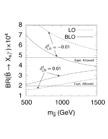
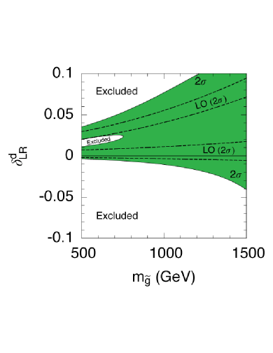
Figure 1: Plots depicting the effect of varying $m_{\widetilde{g}}$ on $\mathrm{BR}(\bar{B}\to X_{s}\gamma)$ (the left panel) and the constraints from $\mathrm{BR}(\bar{B}\to X_{s}\gamma)$ on the insertion $\delta_{LR}^{d}$ (the right panel). In both panels the experimentally allowed range of $\mathrm{BR}(\bar{B}\to X_{s}\gamma)$ is taken at $2\sigma$. In the right panel the allowed regions corresponding to a BLO calculation are shaded in dark green (dark grey) and bounded by solid lines. The equivalent regions corresponding to LO calculation is bounded by dashed lines with no additional shading. In both panels the soft sector is parameterised as follows $m_{\widetilde{q}}=1\,\mbox{TeV}$, $m_{A}=\mu=-A_{u}=500\,\mbox{GeV}$ and $\tan\beta=40$.

The first process we shall consider is $\bar{B}\to X_{s}\gamma$. Before discussing the impact of the current constraint on all four insertions, let us first revisit the focusing effect [13] that exists for the decay in the large $\tan\beta$ regime. Such a situation is illustrated in Fig. 1 where we show the results of a LO and a BLO analysis beside one another for the insertion $\delta_{LR}^{d}$. As is clear from the plots, the difference between the two calculations tends to be rather large. In the left panel we show the variation of the branching ratio on $m_{\widetilde{g}}$ for fixed $\delta_{LR}^{d}$. As is evident from the figure, for positive and negative $\delta_{LR}^{d}$ the BLO calculation leads to values of the branching ratio that are far more compatible with the current experimental and SM results. As discussed in [13, 14, 15], this is mainly due to a cancellation that occurs between the gluino contribution to the decay (that tends to be reduced by BLO corrections) and the BLO corrections to the chargino contribution. This cancellation substantially reduces the SUSY contribution to the decay and leads to the large reductions in the lower limit on $m_{\widetilde{g}}$ evident in the figure.

The implications the focusing effect has on the limits that can be placed on the insertion are illustrated in the right panel, where we show the $2\sigma$ contours in agreement with the experimental result for $\mathrm{BR}(\bar{B}\to X_{s}\gamma)$ (1) in the $\delta_{LR}^{d}-m_{\widetilde{g}}$ plane for a LO and a BLO analysis. As is evident from the figure the difference between the two calculations can be large and the bounds placed on the insertion can be relaxed substantially.

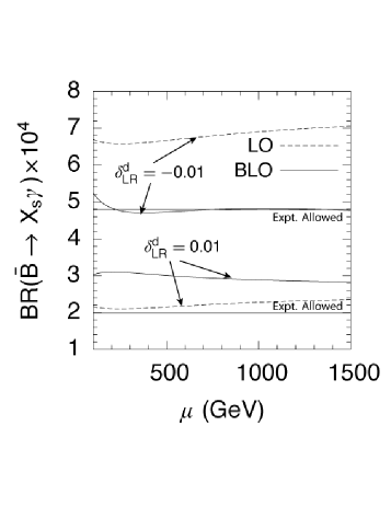
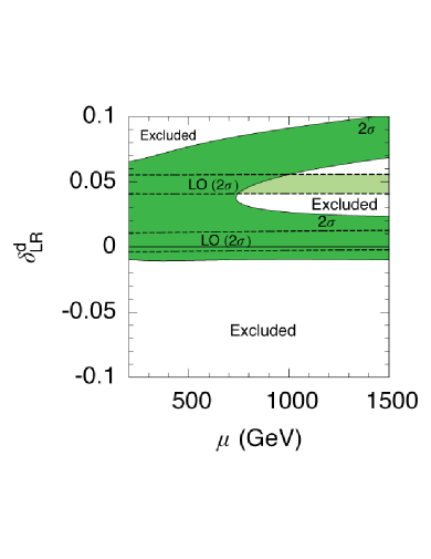
Figure 2: Plots depicting the effect of varying $\mu$ on the constraint supplied by $\bar{B}\to X_{s}\gamma$. In both panels the experimentally allowed range of $\mathrm{BR}(\bar{B}\to X_{s}\gamma)$ is taken at $2\sigma$. In the left panel the branching ratio for the decay is plotted against $\mu$. In the right panel, contours corresponding to the $2\sigma$ limits on the branching ratio for BLO and LO calculations are shown. The regions for a BLO calculation in agreement (at $2\sigma$) with the experimentally allowed range of $\mathrm{BR}(\bar{B}\to X_{s}\gamma)$ are shaded in dark green (dark grey) and bounded by solid lines. The equivalent regions for a LO calculation are bounded by dashed lines with no additional shading when they coincide with the allowed region corresponding to a BLO calculation and by light green (light grey) otherwise. In both panels the soft sector is parameterised as follows $m_{\widetilde{q}}=m_{\widetilde{g}}=1\,\mbox{TeV}$, $m_{A}=-A_{u}=500\,\mbox{GeV}$ and $\tan\beta=40$.

It is natural to ask how, for fixed $m_{\widetilde{q}}$ and $m_{\widetilde{g}}$, the remaining free parameters affect the focusing effect at large $\tan\beta$. The largest contribution to the focusing effect usually arises from the cancellation that takes place between the gluino and BLO chargino contributions to the decay. Regions of parameter space that maximise the chargino contribution to the decay with respect to the gluino contribution would therefore be expected to lead to regions where the focusing effect is greatest. As the squark masses essentially enter the gluino and chargino contributions to the decay, the only difference between the two stems from the appearance of the chargino masses rather than the gluino mass in the relevant matching conditions. The focusing effect is therefore usually maximised when the two masses that enter the diagonal terms of the chargino mass matrix, namely $M_{2}$ and $\mu$ are much smaller than $m_{\widetilde{g}}$. While the soft mass $M_{2}$ is typically lighter than the gluino mass in most SUSY breaking models, the $\mu$ term on the other hand can be much more variable. One should note that whilst increasing $\mu$ will often decrease the BLO chargino correction, it tends to similarly decrease the gluino contribution to the decay through its dependence on the BLO correction $\epsilon_{s}$ (for the relevant expression see Eq. (4.15) in [15]). This compensation tends to reduce the overall $\mu$ dependence of the focusing effect.

The $\mu$ dependence of the branching ratio is presented in the left panel in Fig. 2. As shown in the discussion above, increasing $\mu$ tends to have relatively little impact on the branching ratio. This is caused by the interplay between the BLO corrections to the gluino and chargino contributions mentioned earlier. Similar behaviour is exhibited for RL and RR insertions. For LL insertions, on the other hand, the $\mu$ dependence is slightly more variable as a chargino mediated contribution exists at LO (unlike the other three insertions). Turning to the right panel, we show the bounds on the insertion $\delta_{LR}^{d}$ and how they vary with $\mu$. As is evident from the plot, in contrast to the right panel of Fig. 1, the bounds on the insertion tend to become more stringent with incerasing $\mu$. However, we should point out that, even in regions of parameter space where $\mu>m_{\widetilde{g}}$, the differences between BLO and LO calculations can still be large.

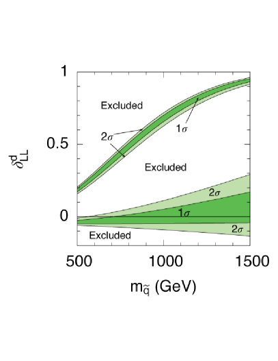
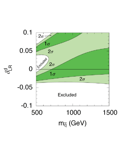
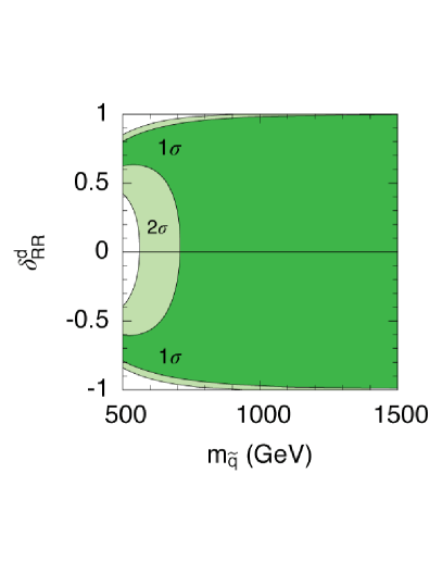
Figure 3: Contour plots depicting the impact of $\mathrm{BR}(\bar{B}\to X_{s}\gamma)$ on the $m_{\widetilde{q}}$—$\delta_{XY}^{d}$ plane. In each plot the soft sector is described as follows $m_{\widetilde{g}}=\sqrt{2}m_{\widetilde{q}}$, $A_{u}=-m_{\widetilde{q}}$, $\mu=m_{\widetilde{q}}/\sqrt{2}$, $m_{A}=500\,\mbox{GeV}$ and $\tan\beta=40$. The light green (light grey) regions highlight areas that agree within $2\sigma$ with the experimental result, the dark green (dark grey) regions within $1\sigma$.

The bounds on each flavour violating parameter imposed by the decay at large $\tan\beta$ are illustrated in Fig. 3. In the top left panel, depicting the limits on the insertion $\delta_{LL}^{d}$, we can see that the bounds are fairly strict. This is because, at leading order, two large contributions to the decay appear. The first is associated with gluino exchange, where the dominant contribution stems from the $\tan\beta$ enhanced correction that appears at second order in the MIA. The second is associated with chargino exchange. As flavour violation between left handed squarks in the up and down sectors is related by $\mathrm{SU}(2)$ symmetry, it is likely that, if $\delta_{LL}^{d}$ is non–zero, the corresponding measure in the up–squark sector – $\delta_{LL}^{u}$ – is non–zero as well. If $\delta_{LL}^{u}$ is non–zero, it is possible to induce a LO contribution via chargino exchange that benefits from appearing at first order in the MIA as well as being $\tan\beta$ enhanced (for a complete set of analytic expressions see [15]). The presence of this LO chargino contribution tends to negate a large part of the focusing effect as it interferes with the cancellation between the BLO part of the chargino contribution, that is proportional to $\delta_{LL}^{d}$, and the LO gluino contribution. As such, even once BLO corrections are taken into account, the impact of the $\bar{B}\to X_{s}\gamma$ constraint on LL insertions at large $\tan\beta$ tends to be more stringent than the other three insertions.

In the top–right panel the bounds on the insertion $\delta_{LR}^{d}$ are illustrated. As is evident from the plot, the bounds on the insertion are fairly weak. This is primarily due to the focusing effect discussed earlier in this section. At LO the constraints on the insertion $\delta_{LR}^{d}$ are more strict (see, for example, the plot on the right of Fig. 1) due to the chiral enhancement $m_{\widetilde{g}}/m_{b}$ the leading order contribution receives. However, once one includes the dominant effects that appear BLO, cancellations between the LO gluino contribution and the BLO corrections to the chargino contribution can lead to a significant relaxation of the bounds on the insertion.

The lower–left and right panels illustrate the bounds imposed on the insertions $\delta_{RL}^{d}$ and $\delta_{RR}^{d}$. As is evident from the plots the bounds derived from $\bar{B}\to X_{s}\gamma$ on these two insertions are rather slight. This is due to the fact that the contributions due to the two insertions cannot interfere with the SM contribution as the dominant contributions due to the insertions are to the primed Wilson coefficients. The bounds on each insertion are therefore fairly symmetric. For the insertion $\delta_{RL}^{d}$ the BLO correction to the charged Higgs vertex arising from higgsino exchange leads to slight deviations from this behaviour [15].

As an aside let us briefly discuss the decoupled limit $m_{\widetilde{q}},m_{\widetilde{g}}\to\infty$ where we are effectively left with a two Higgs doublet model that includes the $\tan\beta$ enhanced threshold corrections discussed in detail in [15]. In this limit the insertions $\delta_{LR}^{d}$ and $\delta_{RL}^{d}$, which scale as $1/M_{SUSY}$, are naturally tiny, and the only meaningful constraint $\bar{B}\to X_{s}\gamma$ can place on sources of SUSY flavour violation is on the insertions $\delta_{LL}^{d}$ and $\delta_{RR}^{d}$. For the insertion $\delta_{LL}^{d}$, the threshold corrections to the charged Higgs vertex can lead to useful bounds that can compliment the constraints supplied by $\bar{B}_{s}\to\mu^{+}\mu^{-}$ and $\bar{B}_{s}-B_{s}$ mixing rather well. For the insertion $\delta_{RR}^{d}$, on the other hand, the corrections to the charged Higgs vertex only affect the primed Wilson coefficients and the constraints that can be imposed on the insertion are rather mild to say the least. We shall discuss this issue further at the end of section 6.

Finally, let us discuss the scenario $\mu<0$. Generally in MFV the $\bar{B}\to X_{s}\gamma$ constraint for $\mu<0$ tends to be fairly stringent as the chargino and charged Higgs contributions interfere constructively with the SM result. In the GFM scenario, on the other hand, this situation can be avoided by inducing relatively mild GFM corrections that interfere destructively with the other SUSY contributions. For $\mu<0$ it is therefore possible to reconcile SUSY contributions with experiment for either negative LL insertions or positive LR insertions. As the negative $\mu$ case was discussed in [13, 14] (see, for example, Fig. 12 of [14]) we shall not cover it in detail here, however, we shall return to it later when we supplement the $\bar{B}\to X_{s}\gamma$ constraint with those provided by $\bar{B}_{s}\to\mu^{+}\mu^{-}$ and $\bar{B}_{s}-B_{s}$ mixing.

4 Limits from $\bar{B}_{s}\to\mu^{+}\mu^{-}$

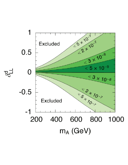
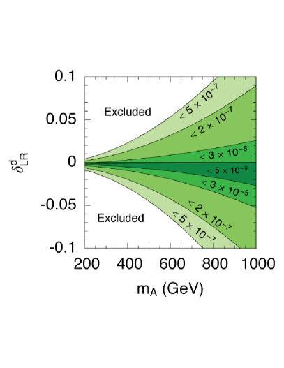
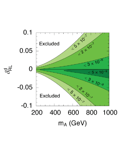
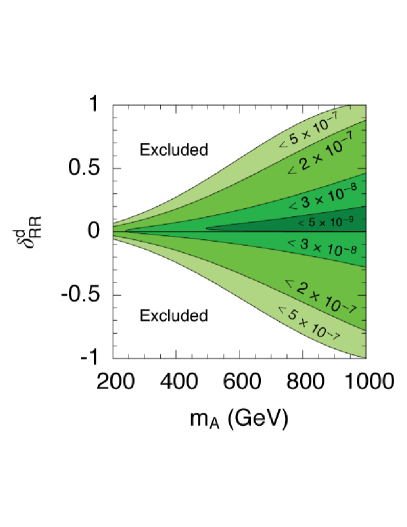
Figure 4: Contour plot depicting the regions of parameter space excluded by increasing the limit on $\mathrm{BR}(\bar{B}_{s}\to\mu^{+}\mu^{-})$ for $\tan\beta=40$. The various shaded regions correspond to regions that satisfy the following upper limits: $5\times 10^{-7}$ light green (light grey); $2\times 10^{-7}$ light–medium green (light–medium grey); $3\times 10^{-8}$ dark–medium green (dark–medium grey) and $5\times 10^{-9}$ dark green (dark grey). The soft sector is parameterised as follows $m_{\widetilde{q}}=m_{\widetilde{g}}=1\,\mbox{TeV}$ and $\mu=-A_{u}=500\,\mbox{GeV}$.

It is well known that SUSY threshold corrections to the neutral Higgs vertex can lead the branching ratio for the decay $\bar{B}_{s}\to\mu^{+}\mu^{-}$ to vary as $\tan^{6}\beta$ [10, 11, 12]. Coupled with a relatively weak dependence on the SUSY mass scale (the branching ratio varies as $1/m_{A}^{4}$ rather than $1/M_{SUSY}^{4}$), the constraint supplied by the Tevatron upper bounds on the decay can prove to be useful even when the coloured SUSY particles (i.e. the squarks and gluino) are heavy.

Figure 4 illustrates the bounds imposed by the decay on each of the insertions for  TeV scale squark masses and varying pseudoscalar Higgs mass in the large $\tan\beta$ regime. All four plots illustrate the useful bounds that can be placed on SUSY flavour violation using the decay, if $m_{A}$ is relatively small (compared to the mass of the squarks).

Before discussing the other aspects of the figures, let us briefly provide a rough recipe that allows those investigating flavour violating effects in the squark sector to decide whether the $\bar{B}_{s}\to\mu^{+}\mu^{-}$ constraint is relevant to their study or not:

$$\lvert\delta_{LL}^{d}\rvert \approx 0.35\left(\frac{40}{\tan\beta}\right)^{3}\left(\frac{500\,\,\mbox{GeV}}{m_{A}}\right)^{-2}; \lvert\delta_{LR}^{d}\rvert \approx 0.026\left(\frac{40}{\tan\beta}\right)^{3}\left(\frac{500\,\,\mbox{GeV}}{m_{A}}\right)^{-2};$$ (15)

$$\lvert\delta_{RL}^{d}\rvert \approx 0.030\left(\frac{40}{\tan\beta}\right)^{3}\left(\frac{500\,\,\mbox{GeV}}{m_{A}}\right)^{-2}; \lvert\delta_{RR}^{d}\rvert \approx 0.26\left(\frac{40}{\tan\beta}\right)^{3}\left(\frac{500\,\,\mbox{GeV}}{m_{A}}\right)^{-2}.$$ (16)

Let us note that these formulae are highly approximate and serve only as a rough guide and should not replace the limits derived from a full numerical analysis.

The effect of improving the limit on $\bar{B}_{s}\to\mu^{+}\mu^{-}$ is also shown in Figure 4. It can be seen from all four plots that even the transition from the published DØ result (4) to the preliminary CDF (5) result reduces the allowed region in the GFM parameter space by a sizeable amount. It is also apparent from the figure that an improvement of the limit to roughly $3\times 10^{-8}$ (a limit achievable at the Tevatron) will provide an excellent constraint on GFM in the large $\tan\beta$ regime. Finally, let us point out the cancellations that can occur for each insertion. For flavour violation in the LL and LR sectors, direct interference with the MFV contributions is possible and values for the branching ratio approaching the SM model value are possible for $m_{A}$ as low as $200\,\mbox{GeV}$, or less. For flavour violation in the RL and RR sectors, on the other hand, the cancellations that can occur are more complicated. In general, the insertions act to increase the branching ratio. However, at large $m_{A}$ regions comparable to the SM can become viable. These regions appear due to a cancellation, between the Wilson coefficients $C_{P}^{\prime}$ and $C_{10}$, that arises when one calculates the branching ratio for the decay. It should be noted that in all four panels the MFV contribution (i.e. all $\delta_{XY}^{d}=0$) is such that SM–like values of the branching ratio are impossible. This is, of course, due to the choice of parameters we make, rather than being a general feature of the MFV contribution at large $\tan\beta$.

The plots in Fig. 4 also serve to illustrate how a lower bound on the pseudoscalar mass derived from the upper limits on BR$\left(\bar{B}_{s}\to\mu^{+}\mu^{-}\right)$ is sensitive to the assumed flavour structure, and how any upper limit that appears (should $\bar{B}_{s}\to\mu^{+}\mu^{-}$ be observed at the Tevatron for example) might be altered beyond MFV. As an example let us consider the top–left and bottom–right panels in Fig. 4. The top–left panel illustrates that one can typically avoid the lower bound on $m_{A}$ altogether even for a relatively minor amount of flavour violation in the LL sector. While this assumption smacks of fine–tuning, one should remember that LL insertions are by far the easiest to generate through RG running in the MSSM (see, for example [28]), and such notions, therefore, might not be as distasteful as one might initially think. Beyond these cancellations that appear for small $\delta_{LL}^{d}$ it is apparent from both panels that the presence of flavour mixings in the squark sector generally act to increase the lower bound on $m_{A}$.

It was discussed in [29] that if one assumed MFV and imposed an upper bound on $\tan\beta$, it would be possible to place some sort of upper bound on the pseudoscalar Higgs mass $m_{A}$. If one allows for GFM in the squark sector it is apparent from all four plots that this result will no longer hold (one can travel along a given band in the plots towards arbitrarily large $m_{A}$) and one would probably need to resort to a more general analysis that takes into account a variety of other processes before any concrete bound could be derived.

5 Limits from $\bar{B}_{s}-B_{s}$ Mixing

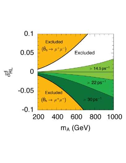
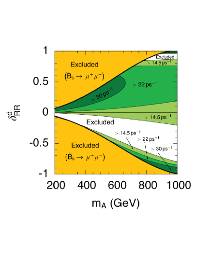
Figure 5: Plots illustrating the dependence on $m_{A}$ and $\delta_{XY}^{d}$ of $\Delta M_{B_{s}}$ once the published DØ limit $\mathrm{BR}(\bar{B}_{s}\to\mu^{+}\mu^{-})<5.0\times 10^{-7}$ has been taken into account (the region shaded in orange/medium grey and bounded by a thick line). The shading is as follows: white regions are excluded by the lower limit $\Delta M_{B_{s}}>14.5\,\mbox{ps}^{-1}$; light green (light grey) regions indicate values of $\Delta M_{B_{s}}$ in the interval $14.5$–$22\,\mbox{ps}^{-1}$; medium green (medium grey) $22$–$30\,\mbox{ps}^{-1}$; dark green regions (dark grey) indicate points in parameter space where $\Delta M_{B_{s}}>30\,\mbox{ps}^{-1}$. The soft sector is parameterised in the same manner as Fig. 4.

Large contributions to $\bar{B}_{s}\to\mu^{+}\mu^{-}$ have been known for some time now to induce similar corrections in the $\bar{B}_{s}-B_{s}$ mixing system. These corrections arise through Feynman diagrams that feature two of the flavour changing neutral Higgs penguin vertices that feature in the $\tan\beta$ enhanced contributions to $\bar{B}_{s}\to\mu^{+}\mu^{-}$ (see [15] for more details). In the MFV scenario such corrections typically lead to reductions to $\Delta M_{B_{s}}$ taking it closer to the current experimental limit [30]. Since LL insertions affect the corrected neutral Higgs vertex in a similar manner to the MFV corrections [15] the overall effect is similar to that found in MFV. The only exception is that the effects are generally more exaggerated due to the enhancement that the GFM correction receives due to the presence of the strong coupling constant in the relevant matching conditions. On the other hand, the contributions due to the insertion $\delta_{LR}^{d}$ tend to be small and generally are bounded by the $\bar{B}_{s}\to\mu^{+}\mu^{-}$ constraint [15].

Turning to flavour violation in the RL and RR sectors, as we pointed out in [15], the contribution where one neutral Higgs penguin is mediated by chargino exchange and the other by gluino exchange (thereby eliminating the suppression by $m_{s}$ that blights the MFV, LL and LR contributions), can yield large effects on $\Delta M_{B_{s}}$. Such effects are illustrated in Fig. 5 where we show contours of $\Delta M_{B_{s}}$ for varying $\delta_{RL}^{d}$, $\delta_{RR}^{d}$ and $m_{A}$ for large $\tan\beta$. As is evident from both panels there is far more variation in $\Delta M_{B_{s}}$ compared to the MFV limit $\delta_{XY}^{d}=0$. Negative values of $\delta_{RR}^{d}$ and positive values $\delta_{RL}^{d}$, in particular, seem to be disfavoured by the current lower bound on $\Delta M_{B_{s}}$. It should be noted that the effects induced by varying $\delta_{RL}^{d}$ arise entirely from BLO corrections and would be absent in a purely LO calculation [15]. From the plots it should also be noted that values for $\Delta M_{B_{s}}$ far in excess of the SM prediction (9) are also allowed by the current upper bound on BR$\left(\bar{B}_{s}\to\mu^{+}\mu^{-}\right)$. This provides a unique signature for the existence of flavour violation in the RR and RL sectors if $\tan\beta$ is large. For example, if the Tevatron were to measure $\mathrm{BR}(\bar{B}_{s}\to\mu^{+}\mu^{-})$ at a level far in excess of the SM prediction, and $\Delta M_{B_{s}}$ was subsequently measured at a value substantially larger than the SM prediction (rather than lower as predicted by MFV [30]), such observations could only point towards the existence of non–minimal flavour structure in either the RL or RR sectors.

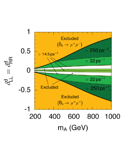
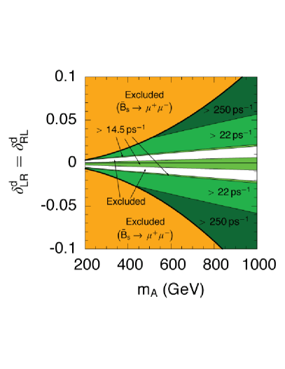
Figure 6: Plots illustrating the variation of $\Delta M_{B_{s}}$ once the published DØ limit $\mathrm{BR}(\bar{B}_{s}\to\mu^{+}\mu^{-})<5.0\times 10^{-7}$ has been taken into account (the region shaded in orange/medium grey and bounded by a thick line). The panels are shaded as follows: white regions are excluded by the lower limit $\Delta M_{B_{s}}>14.5\,\mbox{ps}^{-1}$; light green (light grey) regions indicate values of $\Delta M_{B_{s}}$ in the interval $14.5\,\mbox{ps}^{-1}$–$22\,\mbox{ps}^{-1}$; medium green (medium grey) $22\,\mbox{ps}^{-1}$–$250\,\mbox{ps}^{-1}$; and dark green (dark grey) regions indicate points in paramter space where $\Delta M_{B_{s}}>250\,\mbox{ps}^{-1}$. The soft sector is parameterised in the same manner as Fig. 4.

It has been known for some time [11, 15] that if flavour mixings appear in both the LL and RR sectors then the contributions to $\Delta M_{B_{s}}$ can be especially large. Such a situation is depicted in the left panel in Fig. 6. Here we can see regions where $\Delta M_{B_{s}}$ exceeds values of $250\,\mbox{ps}^{-1}$ (a value unobservable at LHCb) and still satisfies the current published DØ bound $\mathrm{BR}(\bar{B}_{s}\to\mu^{+}\mu^{-})<5.0\times 10^{-7}$. Similar contributions arise if flavour mixings appear in both the LR and RL sectors as illustrated in the right panel in the figure. Here the constraints and the general behaviour of the panel arise only when one includes effects that appear beyond the leading order. (One should note, however, that we do not include the constraint supplied by $\bar{B}\to X_{s}\gamma$ in both panels.) The large contributions that appear in both panels only arise if flavour violation in the LL or LR sectors occur together with flavour violation in the RL or RR sectors.

6 Limits on Single Sources of Flavour Violation

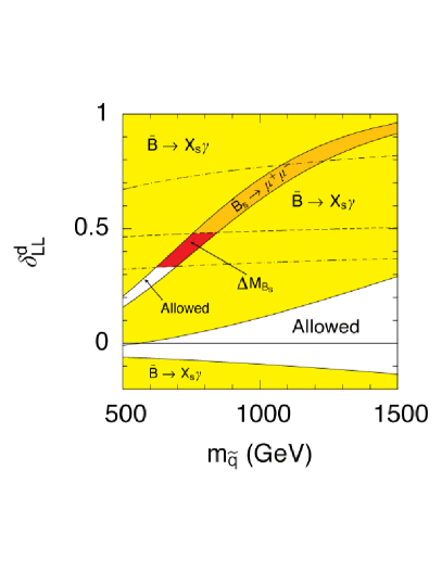
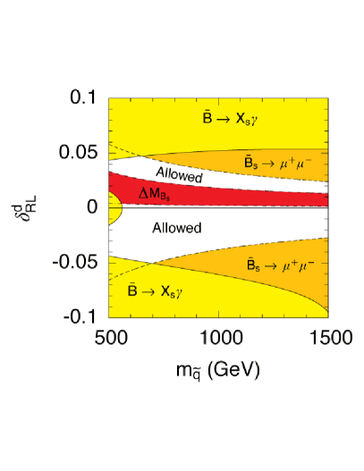
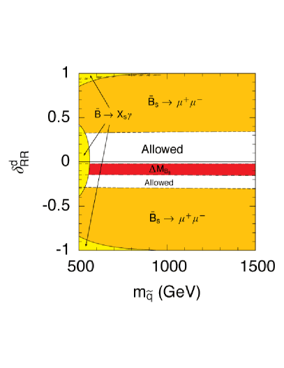
Figure 7: Contour plots showing the current limits on the GFM parameters $\delta_{XY}^{d}$ for varying $m_{\widetilde{q}}$ and fixed $m_{A}$. The soft sector is parameterised in a similar manner to Fig. 3. Regions excluded by $\bar{B}\to X_{s}\gamma$ are shaded in yellow (light grey), the subsequent regions that are excluded by $\bar{B}_{s}\to\mu^{+}\mu^{-}$ are shaded in orange (medium grey), finally the remaining regions that are excluded by the limit on $\Delta M_{B_{s}}$ are shaded in red (dark grey).

With the limits that can be provided by each process in mind, let us now combine all three constraints discussed above. Such a situation is shown in Fig. 7 where we vary $m_{\widetilde{q}}$ along with a single insertion. Unlike the figures shown in the previous three sections we use white to depict allowed regions in parameter space (rather than green/grey) and choose instead to shade the regions excluded by each successive constraint we impose.

The top–left panel in the figure illustrates the allowed parameter space for the insertion $\delta_{LL}^{d}$. It is evident from the figure that the constraints supplied by $\bar{B}_{s}\to\mu^{+}\mu^{-}$ and $\bar{B}_{s}-B_{s}$ mixing play a useful rôle in constraining large values of $\delta_{LL}^{d}$. In particular, they tend to rule out the extreme regions of parameter space, where the SUSY contributions to $\bar{B}\to X_{s}\gamma$ have effectively flipped the sign of the underlying amplitude relative to the SM result. It is also apparent that, when one inspects the contours that outline the regions allowed by these constraints, both processes display a weak dependence on $m_{\widetilde{q}}$. This is due to the decoupling effect of the SUSY corrections to the neutral Higgs vertex [10, 11, 12]. These constraints will therefore remain even when $m_{\widetilde{q}}$ approaches values for in excess of $1\,\mbox{TeV}$ (provided that $m_{A}$ remains constant).

The constraints on the insertion $\delta_{LR}^{d}$ are illustrated in the top–right panel. In this plot we see the constraint supplied by $\bar{B}_{s}\to\mu^{+}\mu^{-}$ once again tends to disfavour larger values of $\delta_{LR}^{d}$. It is also apparent from the plot that the constraint seems to become more severe with increasing $m_{\widetilde{q}}$. This behaviour can be readily understood by recalling that the insertion $\delta_{LR}^{d}$ scales as $1/M_{SUSY}$. If one were to take into account this behaviour somehow, by plotting the constraints on the off–diagonal elements of the actual trilinear soft terms, for example, the correct decoupling behaviour would be restored.

The bottom–left plot in Fig. 7 illustrates the constraints on the insertion $\delta_{RL}^{d}$. Here we see that the processes $\bar{B}_{s}\to\mu^{+}\mu^{-}$ and $\bar{B}_{s}-B_{s}$ remove additional ranges of $\delta_{RL}^{d}$ for $m_{\widetilde{q}}$ as small as $550\,\mbox{GeV}$ and determine the limits on the insertion completely above $m_{\widetilde{q}}\sim 700\,\mbox{GeV}$. Once again the limits imposed by these constraints increase with $m_{\widetilde{q}}$, however, in a similar manner to the insertion $\delta_{LR}^{d}$ discussed above, it is apparent that, once one takes into account the dependence of the insertion on the underlying SUSY mass scale, the correct decoupling will be restored.

Finally, consider the bottom–right panel in the figure that illustrates the bounds on the insertion $\delta_{RR}^{d}$. Here we see that, apart from $m_{\widetilde{q}}\sim 500\,\mbox{GeV}$ – where MFV is disfavoured by the $\bar{B}\to X_{s}\gamma$ constraint, the limits on the insertion are determined completely by the limits on $\mathrm{BR}\left(\bar{B}_{s}\to\mu^{+}\mu^{-}\right)$ and $\Delta M_{B_{s}}$. In addition, in a similar manner to the insertion $\delta_{LL}^{d}$ the dependence of these two constraints on the underlying SUSY mass scale is extremely weak. As such, the constraints supplied by these two processes will continue to be useful, even if the squarks and gluino effectively decouple.

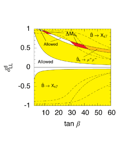
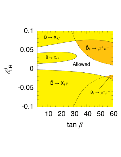
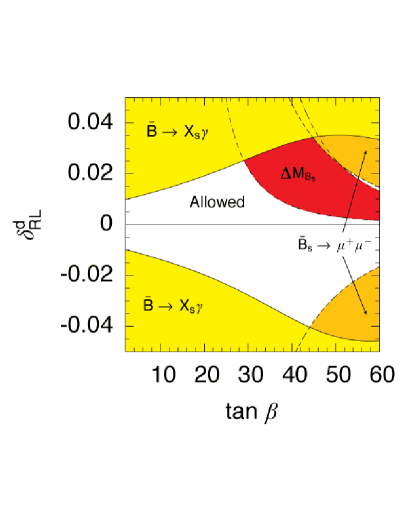
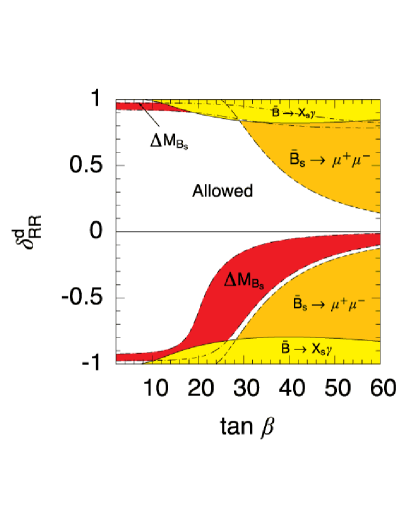
Figure 8: Contour plots showing the limits on the GFM parameters $\delta_{XY}^{d}$ for varying $\tan\beta$. The soft sector is parameterised in a similar manner to Fig. 4 with $m_{A}=500\,\mbox{GeV}$. The excluded/allowed regions are shaded in a similar manner to Fig. 7.

The SUSY contributions to all three processes under investigation in this paper are well known to be highly dependent on $\tan\beta$. The corrections to $\mathrm{BR}\left(\bar{B}_{s}\to\mu^{+}\mu^{-}\right)$ and $\Delta M_{B_{s}}$ for instance scale as $\tan^{6}\beta$ and $\tan^{4}\beta$ while the BLO focusing effect, discussed in [13, 14, 15] and at the beginning of section 3, is also strongly dependent on $\tan\beta$. It is, therefore, natural to ask how the limits on the various sources of flavour violation depend on $\tan\beta$. Such a situation is shown in Fig. 8 where we illustrate the allowed regions in the parameter space formed by varying $\tan\beta$ and one insertion at a time.

In the top–left panel the constraints on the insertion $\delta_{LL}^{d}$ are shown. Here we see that, in contrast to the other three panels in the figure, the constraints on the insertion increase dramatically with $\tan\beta$. For example, at low $\tan\beta$, the insertion is relatively unconstrained and values of up to $\delta_{LL}^{d}\sim 0.8$ are easily possible. This is because the dominant LO chargino and gluino contributions to the decay that arise from LL insertions are both proportional to $\tan\beta$. As $\tan\beta$ increases the constraint imposed by $\bar{B}\to X_{s}\gamma$ therefore becomes much more stringent and separates into two distinct branches. The upper branch here is associated with regions where the amplitude associated with the decay has effectively changed sign. Once we include the constraints supplied by $\bar{B}_{s}\to\mu^{+}\mu^{-}$ and $\bar{B}_{s}-B_{s}$ mixing, however, these extreme regions are typically ruled out for $\tan\beta>30$ (and also, to some extent, for $\tan\beta<15$).

The limits on the insertion $\delta_{LR}^{d}$ are shown in the top–right panel. Here we see the focusing effect rather clearly: the regions of parameter space excluded by the $\bar{B}\to X_{s}\gamma$ constraint decrease dramatically as $\tan\beta$ increases, in contrast to a LO analysis where, essentially, the bounds on $\delta_{LR}^{d}$ are relatively independent of $\tan\beta$. As $\tan\beta$ increases, however, the constraint supplied by the decay $\bar{B}_{s}\to\mu^{+}\mu^{-}$ also gains prominence and becomes important in determining the limits on the insertion above $\tan\beta\sim 30$. Indeed, above $\tan\beta\sim 55$, the constraints on $\delta_{LR}^{d}$ are determined entirely by the published DØ bound $\mathrm{BR}(\bar{B}_{s}\to\mu^{+}\mu^{-})<5.0\times 10^{-7}$.

The lower–left panel in the figure illustrates the bounds on the flavour violation in the RL sector. Once again, the bounds on the insertion supplied by the $\bar{B}\to X_{s}\gamma$ constraint decrease steadily as $\tan\beta$ increases. This is due to the focusing effect discussed at the beginning of section 3. It is also apparent from the figure that the constraints supplied by $\bar{B}_{s}\to\mu^{+}\mu^{-}$ and $\bar{B}_{s}-B_{s}$ mixing play large rôles when determining the limits on $\delta_{RL}^{d}$ at large $\tan\beta$. The limits imposed by the current lower bound on $\Delta M_{B_{s}}$, for instance, start eliminating large regions of parameter space for positive $\delta_{RL}^{d}$ for $\tan\beta$ as low as $30$. Increasing $\tan\beta$ only serves to increase the effectiveness of the constraints supplied by the decay $\bar{B}_{s}\to\mu^{+}\mu^{-}$ and $\bar{B}_{s}-B_{s}$ mixing, and, for example, above $\tan\beta\sim 45$ the constraint provided by $\bar{B}\to X_{s}\gamma$ is entirely supplanted by those attributable to $\bar{B}_{s}\to\mu^{+}\mu^{-}$ and $\bar{B}_{s}-B_{s}$ mixing.

Finally, in the bottom–right panel we show the limits on the insertion $\delta_{RR}^{d}$. From the plot it is evident that the bounds imposed by $\bar{B}\to X_{s}\gamma$ are fairly weak. This is principally due to two reasons: the first is that the insertion $\delta_{RR}^{d}$ only contributes (in a significant manner) to the primed Wilson coefficients and, therefore, cannot interfere directly with the SM contribution; the second is that the BLO focusing effect significantly reduces the $\tan\beta$ enhanced LO contribution that arises from gluino exchange. It is therefore apparent from the figure that the constraints supplied by both $\bar{B}_{s}\to\mu^{+}\mu^{-}$ and $\bar{B}_{s}-B_{s}$ can become important even for $\tan\beta$ as low as $20$ and for $\tan\beta>30$ the constraints on the insertion are determined entirely by these two processes.

$\delta_{LL}^{d}(10^{-2})$	$\tan\beta=10$	$\tan\beta=40$	$\tan\beta=50$
A	$(-2.2,11.0),\,(47,56)$	$(-4,11)$	$[-1.2,-0.2)$
B	$(-10,40)$	$(-7,10)$	$(-7.4,8.0)$
C	$(-5,8.6),\,(45.6,54.8)$	$(-4.4,0.2),\,(14.4,18.8)$	$(-4.6,-0.7),\,(12.0,15.8)$
D	$(-17.4,37.0)$	$(-9.2,9.6)$	$(-8.8,7.4)$
$\delta_{LR}^{d}(10^{-3})$	$\tan\beta=10$	$\tan\beta=40$	$\tan\beta=50$
A	$(-1.2,7.6),\,(22,31)$	$(-12,2)$	$[-9.2,-1.6)$
B	$(-3,15),\,(46,64)$	$(-12,18)$	$[-14.8,9.2]$
C	$(-3.0,5.4),\,(21.0,29.6)$	$(-13.4,0.2),\,(26.4,33.6]$	$(-19.2,-3.6)$
D	$(-5.00,12.8),\,(45.0,63.0)$	$(-14.8,19.6),\,(55.2,78.8]$	$(-20.2,24.4)$
$\delta_{RL}^{d}(10^{-3})$	$\tan\beta=10$	$\tan\beta=40$	$\tan\beta=50$
A	$(-7.0,7.0)$	$[-12,0.5\},\,\{6,10]$	Excl.
B	$(-16,16)$	$[-30,2\},\,\{14,26]$	$[-16.0,0.6\},\,\{6.6,14.0]$
C	$(-9.8,9.8)$	$(-32.8,3.4\},\,\{26.2,32.0)$	$[-28.0,-15.0),\,(13.8,24.8]$
D	$(-19.4,19.4)$	$(-52.8,7.6\}$	$[-64.4,3.4\},\,\{27.6,57.2]$
$\delta_{RR}^{d}(10^{-2})$	$\tan\beta=10$	$\tan\beta=40$	$\tan\beta=50$
A	$(-24.6,26.8)$	$[-5,-2\},\,\{-0.4,6]$	Excl.
B	$(-80,84)$	$[-23.2,-11.4\},\,\{-1.6,26.4]$	$[-13.0,-6.0\},\,\{-0.6,14.8]$
C	$(-36.4,38.6)$	$[-22.6,-11.6\},\,\{-1.6,25.8]$	$[-12.6,-6.1\},\,(9.4,14.6]$
D	$\{91.2,92.0\}$	$(-71.4,-39.2\},\,\{-6.4,74.2)$	$[-50.8,-21.8\},\,\{-3.1,56.8]$

Table 1: Table of limits on all four insertions for varying $\tan\beta$. The soft sector is parameterised as follows: in all four scenarios $m_{\widetilde{q}}=m_{\widetilde{g}}=\mu$ and $A_{u}=-m_{\widetilde{q}}$; in scenarios A and C $m_{\widetilde{q}}=500\,\mbox{GeV}$; in scenarios B and D $m_{\widetilde{q}}=1\,\mbox{TeV}$. The pseudoscalar mass $m_{A}$ is given by $m_{A}=m_{\widetilde{q}}/2$ in scenarios A and B, and by $m_{A}=m_{\widetilde{q}}$ for scenarios C and D. The source of each bound is indicated by varying styles of bracket, conventional round brackets indicate $\bar{B}\to X_{s}\gamma$, square brackets $\bar{B}_{s}\to\mu^{+}\mu^{-}$ and braces indicate $\bar{B}_{s}-B_{s}$ mixing.

To illustrate the usefulness of combining the constraints supplied by $\bar{B}\to X_{s}\gamma$, $\bar{B}_{s}\to\mu^{+}\mu^{-}$ and $\bar{B}_{s}-B_{s}$ mixing we provide a list of the bounds on each insertion in table 1. The first column in the table illustrates the bounds on the insertions for $\tan\beta=10$. It is evident here that, for this moderate value of $\tan\beta$, the constraints on all four insertions are determined entirely by the decay $\bar{B}\to X_{s}\gamma$ (except for one case for $\delta_{RR}^{d}$). This is, of course, to be expected due to the large dependence the neutral Higgs penguin contributions to $\bar{B}_{s}\to\mu^{+}\mu^{-}$ and $\Delta M_{B_{s}}$ have on $\tan\beta$. Moving on to the next two columns which display the limits on the insertions for much larger values of $\tan\beta$ it can be seen that both $\bar{B}_{s}\to\mu^{+}\mu^{-}$ and $\bar{B}_{s}-B_{s}$ mixing play a much more useful rôle. For example, for LL and LR insertions the constraints either remove the second set of allowed values that were present at $\tan\beta=10$ or reduce them somewhat, even for relatively large $m_{A}$. For RL and RR insertions the constraints are determined almost entirely (with one or two exceptions) by the current limits on $\mathrm{BR}\left(\bar{B}_{s}\to\mu^{+}\mu^{-}\right)$ and $\Delta M_{B_{s}}$. The allowed values of these insertions also take a different form compared with those obtained for small $\tan\beta$. For low $\tan\beta$ the allowed regions are usually given by (roughly) symmetric regions centred on the MFV limit (i.e. $\delta_{XY}^{d}=0$). However, at large $\tan\beta$ the allowed regions appear to split into two separate branches. These branches that appear at negative $\delta_{RR}^{d}$ and positive $\delta_{RL}^{d}$ are, essentially, regions of parameter space where the SUSY contributions have flipped the sign of the underlying amplitude, relevant to $\bar{B}_{s}-B_{s}$ mixing, relative to the SM result.

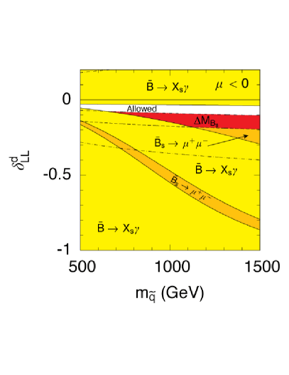
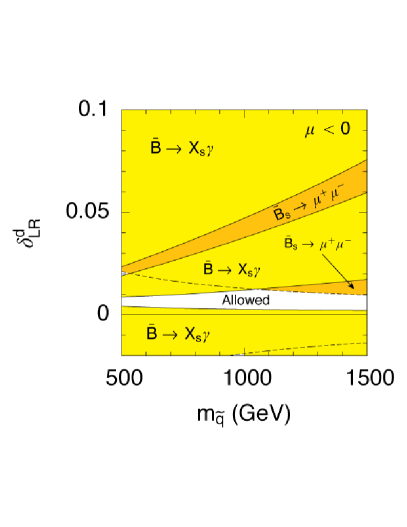
Figure 9: Contour plots showing the current limits on the GFM parameters $\delta_{LL}^{d}$ and $\delta_{LR}^{d}$ for varying $m_{\widetilde{q}}$ and $\mu<0$. The soft sector is parameterised in a similar manner to Fig. 3 while the shading of the figure is that same as Fig. 7.

Let us now consider the case $\mu<0$. As discussed earlier in this paper, for $\mu<0$, the chargino and charged Higgs contributions to $\bar{B}\to X_{s}\gamma$ interfere constructively with the SM result and one is often forced to adopt a very heavy SUSY mass spectrum ($M_{SUSY}\gg 1\,\mbox{TeV}$) to ensure that the contributions to $\mathrm{BR}(\bar{B}\to X_{s}\gamma)$ are not too large. In GFM it is possible to improve the situation by considering contributions from either LL or LR insertions that interfere destructively with the chargino and charged Higgs corrections to the decay. This problem is made somewhat easier when one considers BLO effects as, instead of reducing the GFM contribution, as they do for positive $\mu$, they act to increase it (i.e. “anti–focusing”). As such it is possible that relatively small deviations from MFV will satisfy the $\bar{B}\to X_{s}\gamma$ constraint. As changing the sign of $\mu$ also changes the sign of the term $\epsilon_{s}$ that appears in the various BLO corrections presented in [15], it is apparent that the contributions to both $\bar{B}_{s}\to\mu^{+}\mu^{-}$ and $\bar{B}_{s}-B_{s}$ mixing will increase as well. It is therefore to be expected that the constraints imposed by these two processes will play an even greater rôle compared to the positive $\mu$ case. Such a situation is shown in Fig. 9 where we present the allowed parameter space in the $\delta_{LL}^{d}$–$m_{\widetilde{q}}$ and $\delta_{LR}^{d}$–$m_{\widetilde{q}}$ planes for negative $\mu$. Each plot displays the familiar structure of two branches that are compatible with the $\bar{B}\to X_{s}\gamma$ constraint encountered earlier in Fig. 3. In a similar manner to the plots found in Fig. 7 the constraints supplied by the limits on $\mathrm{BR}(\bar{B}_{s}\to\mu^{+}\mu^{-})$ and $\Delta M_{B_{s}}$ tend to rule out the more extreme regions of parameter space. For example in each figure the constraint supplied $\bar{B}_{s}\to\mu^{+}\mu^{-}$ excludes the extreme branch of the region permitted by $\bar{B}\to X_{s}\gamma$. In the left panel of Fig. 9 the constraint supplied by $\bar{B}_{s}-B_{s}$ mixing also plays a large role and rules out over half of the allowed parameter space in the upper branch in the figure. It is obvious from both figures however that regions consistent with all three constraints are still possible and $\mu<0$ can still be a viable possibility at least when one considers minor departures from MFV.

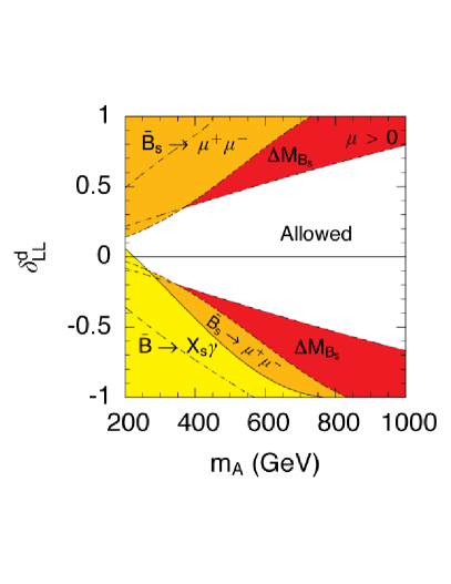
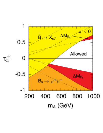
Figure 10: Contour plots depicting the limits on the insertion $\delta_{LL}^{d}$ in the decoupled limit $m_{\widetilde{q}}\gg m_{A}$. The soft sector is parameterised as follows $m_{\widetilde{q}}=\sqrt{2}\mu=m_{\widetilde{g}}/\sqrt{2}=-A_{u}=10\,\mbox{TeV}$ and $\tan\beta=40$. In the left panel $\mu>0$, while in the right panel $\mu<0$.

Finally, let us consider the decoupled limit $m_{\widetilde{q}},m_{\widetilde{g}}\gg m_{A}$. Such a situation is illustrated in Fig. 10 where we depict the constraints that can be placed on the insertion $\delta_{LL}^{d}$. As is evident from the two panels all three processes continue to play a rôle in constraining the LL insertions. It should be noted that the constraints arising from $\bar{B}\to X_{s}\gamma$ in particular, are a purely BLO effect. The constraints arise from the threshold corrections to the charged Higgs vertex and can act to either increase or decrease the contribution to $\bar{B}\to X_{s}\gamma$ arising from charged Higgs exchange relative to a purely LO calculation. This is in contrast to an MFV calculation where the BLO corrections act only to decrease the charged Higgs contribution for $\mu>0$ and increase it for $\mu<0$. It is also evident from both panels that the constraints provided by $\bar{B}_{s}\to\mu^{+}\mu^{-}$ and $\Delta M_{B_{s}}$, which arise from the threshold corrections to the neutral Higgs vertex, continue to play an important rôle eliminating roughly symmetric regions of parameter space in each panel. Finally, let us note that in each panel the lower bound on $m_{A}$ in the MFV limit is determined solely by $\bar{B}\to X_{s}\gamma$, however, once one proceeds beyond this approximation the lower limit on $m_{A}$ can be dictated by either the $\bar{B}_{s}\to\mu^{+}\mu^{-}$ or $\bar{B}_{s}-B_{s}$ constraints (especially when $\mu>0$, as in the left panel).

It is natural to ask how the other insertions are constrained in this extreme region of parameter space. As the threshold corrections to the charged Higgs vertex, arising from RR insertions, only effect the primed Wilson coefficients [15] it is apparent that the constraint supplied by $\bar{B}\to X_{s}\gamma$ will have a relatively minor dependence on $\delta_{RR}^{d}$. As such the constraints on the insertion are usually determined by $\bar{B}_{s}\to\mu^{+}\mu^{-}$ and $\bar{B}_{s}-B_{s}$ mixing, and eliminate regions of parameter space similar to those found in Figs. 4–5. Turning to flavour violation in the LR and RL sectors, as the original definitions for these scale as $1/M_{SUSY}$, it is generally more useful to constrain the actual elements of the trilinear soft terms themselves, or at least a dimensionless quantity that does not feature a Higgs VEV or quark mass. Provided one takes this into account it is apparent from the decoupling behaviour exhibited by the $\bar{B}_{s}\to\mu^{+}\mu^{-}$ and $\bar{B}_{s}-B_{s}$ constraints in Fig. 7 that both processes will continue to be useful when constraining flavour violation in the LR and RL sectors, even for $m_{\widetilde{q}}=10\,\mbox{TeV}$. Turning to the $\bar{B}\to X_{s}\gamma$ constraint, neither insertion induces large threshold corrections to the charged Higgs vertex and as such the dependence of the $\bar{B}\to X_{s}\gamma$ constraint on these two insertions would be expected to be relatively small when compared to the large dependence on $\delta_{LL}^{d}$ exhibited in Fig. 10.

7 Limits on Multiple Sources of Flavour Violation

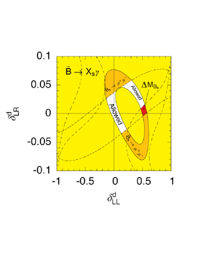
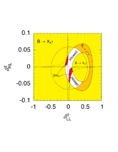
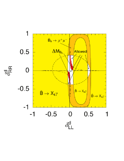
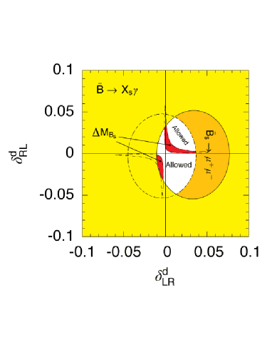
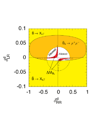
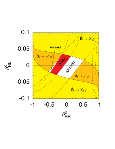
Figure 11: Shading the same as Fig. 7, the soft sector is parameterised in a similar manner to Fig. 4 with $m_{A}=500\,\mbox{GeV}$.

Up until now, for the sake of simplicity, we have been mainly concerned with one source of flavour violation being varied at a time. However, it is more natural to expect more than one insertion to be simultaneously non–zero. This may lead to a more varied picture. For example, as discussed at the end of section 5, large contributions to $\Delta M_{B_{s}}$ are possible if two insertions are both non–zero. Coupled with the possibility that interference between the various contributions can also play a rôle for $\bar{B}\to X_{s}\gamma$ and $\bar{B}_{s}\to\mu^{+}\mu^{-}$, it is interesting to consider the limits attainable if one decides to vary two sources of flavour violation in the squark sector at once. Such a situation is shown in Fig. 11.

First let us consider the regions ruled out by the $\bar{B}\to X_{s}\gamma$ constraint (the yellow regions). The regions permitted by the constraint are typically circular in nature with the exception of the $\delta_{RL}^{d}$–$\delta_{RR}^{d}$ plane (the bottom–right panel). The reason for the deviation is due to the fact that neither insertion contributes significantly to the unprimed Wilson coefficients $C_{7}$ and $C_{8}$ and the overall effect of the insertions is to increase the branching ratio for the decay. For the remaining combinations at least one of the insertions contributes to the unprimed sector and can therefore lead to a decrease as well as increase in BR$(\bar{B}\to X_{s}\gamma)$. Let us briefly also mention why some of the circular regions are filled (mainly those featuring the insertion $\delta_{LR}^{d}$) whilst others are unfilled (those that feature the insertion $\delta_{LL}^{d}$). The reason here is due to the focusing effect discussed at the beginning of section 3. In a similar manner to the top–right panel in Fig. 3, the focusing effect raises the minimum value for $\mathrm{BR}(\bar{B}\to X_{s}\gamma)$ in the circular regions towards the SM value and above the lower limit we impose (a more stringent lower limit would lead to “doughnut” shaped regions like the remaining panels). As the contributions due to LL insertions are less affected by BLO corrections (compared with the other three insertions) the allowed regions in the plots featuring this insertion tend to retain a similar form to their LO counterparts.

All six panels in the figure easily illustrate the usefulness of the current bound in $\bar{B}_{s}\to\mu^{+}\mu^{-}$ in constraining GFM at large $\tan\beta$ (the dashed lines). It is also apparent that the regions excluded by the constraint are rather different in the $\delta_{LL}^{d}$–$\delta_{LR}^{d}$ and the $\delta_{RL}^{d}$–$\delta_{RR}^{d}$ planes (the top–left and bottom–right panels respectively) compared with the remaining four combinations. This is because, in both cases, the contributions to the neutral Higgs penguin interfere directly with one another, leading to the rectangular shaped regions in the two panels. It should also be noted that these regions are orientated at roughly ninety degrees to the $\bar{B}\to X_{s}\gamma$ constraint in both panels. As such, the combination of the two constraints tends to be fairly complementary when constraining these two combinations. For the remaining four contributions, one insertion affects the right–handed Higgs vertex while the other affects the left–handed vertex. These contributions translate to contributions to the unprimed and primed Wilson coefficients respectively. Direct interference is therefore ruled out, resulting in the circular regions found in the remaining four plots.

Let us now consider the constraint imposed by the $\bar{B}_{s}-B_{s}$ mixing system. Here we see that, in all six panels, the constraint imposed by this process is comparatively mild (with the exception of the $\delta_{RL}^{d}$–$\delta_{RR}^{d}$ plane). This is mainly due to the way we impose the constraint. Since we simply require that $\Delta M_{B_{s}}>14.5\,\mbox{ps}^{-1}$ the regions excluded in the panels involving the combination of an LL or an LR insertion, and a RL or a RR insertion, tend to be rather slight due to the large effects that are possible for these combinations (see the end of section 5). Therefore, if one chose to impose some sort of upper bound on $\Delta M_{B_{s}}$ as well, the constraints on SUSY flavour violation imposed by the $\bar{B}_{s}-B_{s}$ mixing system would be far more stringent.

Finally, let us briefly make one more remark concerning how the plots in Fig. 11 might change should one choose to vary other sources of flavour violation in addition to those already being varied in each plot. Generally, it would be expected that quite large deviations from the contours shown in Fig. 11 occur once one proceeds beyond this limit, however, there is one exception. Certain regions in the top–left panel of Fig. 11 are relatively independent of the effects of varying $\delta_{RL}^{d}$ and $\delta_{RR}^{d}$. This is due to the fact that varying $\delta_{RL}^{d}$ and $\delta_{RR}^{d}$ invariably only affects the primed Wilson coefficients. The result of varying these insertions is that they, therefore, tend to increase the values of BR$(\bar{B}\to X_{s}\gamma)$ and BR$(\bar{B}_{s}\to\mu^{+}\mu^{-})$ compared to a calculation where they are set to zero. Varying these insertions might therefore fill in the excluded region at the centre of the “doughnut” shown in the plot. The variation, however, will not affect (in a large manner) the regions excluded by the outer ring that delineates the $\bar{B}\to X_{s}\gamma$ constraint nor the regions excluded by the $\bar{B}_{s}\to\mu^{+}\mu^{-}$ constraint. The regions excluded by the lower bound on $\Delta M_{B_{s}}$, however, will tend to vary much more as varying RL and RR insertions together with LL and LR insertions inevitably leads to large deviations in $\Delta M_{B_{s}}$.

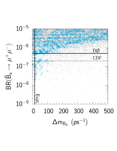
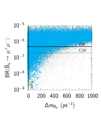
Figure 12: Scatter plots illustrating the relationship between $\mathrm{BR}(\bar{B}_{s}\to\mu^{+}\mu^{-})$ and $\Delta M_{B_{s}}$ when all four sources of flavour violation are being varied. In each plot $\delta_{LL}^{d}$ and $\delta_{RR}^{d}$ are varied over the range $[-0.8,0.8]$, while the insertions $\delta_{LR}^{d}$ and $\delta_{RL}^{d}$ are varied over the range $[-0.08,0.08]$. The soft sector is parameterised using the relations $m_{\widetilde{q}}=-A_{u}=m_{\widetilde{g}}/\sqrt{2}=\sqrt{2}\,\mu=2\,m_{A}$ with $m_{\widetilde{q}}=500\,\mbox{GeV}$ in the left panel and $m_{\widetilde{q}}=1\,\mbox{TeV}$ in right panel, $\tan\beta=40$ in both plots. Blue (grey) squares denote points that are consistent with the experimental result for $\mathrm{BR}(\bar{B}\to X_{s}\gamma)$, while black dots are not.

The correlation between certain observables in the large $\tan\beta$ regime is well known. In [30], for instance, a strong correlation between BR$(\bar{B}_{s}\to\mu^{+}\mu^{-})$ and $\Delta M_{B_{s}}$ was pointed out that exists due to the dependence both processes have on the neutral Higgs penguin. It was shown in [15] that similar correlations exist if one varies only one insertion at a time in the GFM scenario. Fig. 12 illustrates the result of varying all four insertions at the same time, in a particular region of parameter space. As is evident from the figure, the correlation between BR$(\bar{B}_{s}\to\mu^{+}\mu^{-})$ and $\Delta M_{B_{s}}$ that exists in MFV and certain limits of GFM is less pronounced once one varies all four sources of flavour violation. This is hardly surprising once one notices the vastly different behaviour exhibited by the contributions arising from each insertion to $\Delta M_{B_{s}}$ [15], as well as the fact that multiple sources of flavour violation lead to exceptionally large contributions to $\Delta M_{B_{s}}$ (see the end of section 5). The scatter plots in Fig. 12 also demonstrate the effect that increasing the bounds on $\mathrm{BR}(\bar{B}_{s}\to\mu^{+}\mu^{-})$ or $\Delta M_{B_{s}}$ might have on the available parameter space. In the left panel (corresponding to a relatively light SUSY spectrum and Higgs sector) it is evident that the majority of the points consistent with $\bar{B}\to X_{s}\gamma$ have already been ruled out by the Tevatron limits on $\mathrm{BR}(\bar{B}_{s}\to\mu^{+}\mu^{-})$. Turning to the right panel, where the mass spectrum is twice as heavy, it is evident that there is far more freedom, this is of course unsurprising as the contributions to all three processes decrease as the mass spectrum increases. It is evident from the plot, however, that reducing the limit on $\mathrm{BR}(\bar{B}_{s}\to\mu^{+}\mu^{-})$ to roughly $3\times 10^{-8}$ or observing $\Delta M_{B_{s}}$ will affect the available parameter space dramatically.

8 Other Constraints

Before proceeding with our conclusions let us briefly discuss how some additional constraints might affect the available parameter space in the GFM scenario.

The first process we shall consider is the decay $\bar{B}\to X_{s}l^{+}l^{-}$. The effect this process might have on the SUSY parameter space was discussed in [31] where it was shown that the combined constraints provided by $\bar{B}\to X_{s}l^{+}l^{-}$ and $\bar{B}\to X_{s}\gamma$ indicate that the sign of the amplitude for the decay $\bar{B}\to X_{s}\gamma$ was that of the SM, unless large contributions to the Wilson coefficients $C^{\mathrm{eff}}_{9}$ and $C^{\mathrm{eff}}_{10}$ could be induced. Recalling the discussions in section 3 and section 6, it is possible for both LL and LR insertions to induce contributions to $\bar{B}\to X_{s}\gamma$ that flip the sign of the underlying amplitude (see, for example, the upper branches of the top–left and top–right panels in Fig. 3). As we have seen, the constraints imposed by $\bar{B}_{s}\to\mu^{+}\mu^{-}$ and $\bar{B}_{s}-B_{s}$ mixing typically exclude the majority of these regions at large $\tan\beta$. However it is still possible, in some cases, that such regions can remain even after one has taken into account both of these constraints (see, for example, the top–left panel in Fig. 11). In addition, it is interesting to consider how one might remove these regions at low $\tan\beta$ where the $\bar{B}_{s}\to\mu^{+}\mu^{-}$ and $\bar{B}_{s}-B_{s}$ mixing constraints play only a minor rôle. While a complete analysis of the $\bar{B}\to X_{s}l^{+}l^{-}$ constraint in GFM is beyond the scope of this analysis, let us briefly make a few comments on the possible effects of the constraint.

For LR insertions it is difficult to induce large contributions to either $C^{\mathrm{eff}}_{9}$ or $C^{\mathrm{eff}}_{10}$. This is because the operators associated with these Wilson coefficients feature the Dirac bilinear $s_{L}\gamma_{\mu}b_{L}$. The contributions to these operators arising from LR insertions, therefore, appear at second order in the mass insertion approximation and suffer from a suppression by either the strange or bottom quark mass. Compared with the large contributions induced by LR insertions to the Wilson coefficient $C^{\mathrm{eff}}_{7}$ that appear at first order in the MIA, in addition to being chirally enhanced by the gluino mass, it is likely that the constraint imposed by $\bar{B}\to X_{s}l^{+}l^{-}$ will be useful in constraining the large values of LR insertions that have effectively flipped the sign of the $\bar{B}\to X_{s}\gamma$ amplitude, at low $\tan\beta$ in particular.

Turning to LL insertions, it is possible that contributions to the operators associated with the Wilson coefficients $C^{\mathrm{eff}}_{9}$ and $C^{\mathrm{eff}}_{10}$ might be somewhat larger as contributions proportional to $\delta_{LL}^{d}$ can appear at first order in the MIA via photon penguins [32]. These contributions are not enhanced by $\tan\beta$, however, and it seems likely that for large $\tan\beta$ the constraint will play a similar rôle to $\bar{B}_{s}\to\mu^{+}\mu^{-}$ and $\bar{B}_{s}-B_{s}$ mixing, due to the $\tan\beta$ enhancement of the corrections to $C^{\mathrm{eff}}_{7}$. The impact the constraint might have on constraining RL and RR is less clear as they affect the primed coefficients and the possibility of flipping the sign of the $\bar{B}\to X_{s}\gamma$ amplitude is removed.

In summary, in most cases at large $\tan\beta$, the flipped sign of the amplitude for the decay $\bar{B}\to X_{s}\gamma$ is excluded by a combination of the experimental bounds from $\bar{B}_{s}\to\mu^{+}\mu^{-}$ and $\bar{B}_{s}-B_{s}$ mixing. For low values of $\tan\beta$ however, where the constraints provided by $\bar{B}_{s}\to\mu^{+}\mu^{-}$ and $\bar{B}_{s}-B_{s}$ play only a minor rôle, it is clear that the additional constraint provided by $\bar{B}\to X_{s}l^{+}l^{-}$ will be fairly useful when attempting to exclude these extreme regions of parameter space [33].

Another means of constraining the GFM parameters $\delta_{XY}^{d}$ that has been discussed in the literature is via the use of precision electroweak observables, such as $m_{W}$ and $\sin^{2}\theta_{\mathrm{eff}}$ [34]. The constraints in this case typically affect either LL or RR insertions as contributions due to LR and RL insertions typically appear at fourth order in the MIA (as opposed to second order for LL and RR insertions). Taking into account these corrections, it has been shown that, for large values of $\delta_{LL}^{d}$, quite sizeable corrections to both $m_{W}$ and $\sin^{2}\theta_{\mathrm{eff}}$ can be induced that provide a useful limit in constraining extreme values of $\delta_{LL}^{d}$ [34]. The improved measurements that will be made at the LHC and the next linear collider will serve to strengthen these constraints even more.

9 Conclusions

In conclusion we have discussed the current limits that can be placed on SUSY flavour violation. In particular, we have included all the relevant $\tan\beta$ enhanced corrections that appear at BLO when calculating the SUSY contributions to the various processes under consideration. For the decay $\bar{B}\to X_{s}\gamma$ we have reiterated the need to include BLO corrections when deriving limits in the large $\tan\beta$ limit, showing the effect of varying parameters such as $\mu$ and $m_{\widetilde{g}}$ on the BLO focusing effect discussed previously in [13, 14, 15]. For the processes $\bar{B}_{s}\to\mu^{+}\mu^{-}$ and $\bar{B}_{s}-B_{s}$ mixing we have shown that useful limits can be placed on all four insertions with the current experimental bounds. We have also combined the limits from all three processes and investigated the effect the constraints have in a variety of scenarios. In particular, we have shown that both $\bar{B}_{s}\to\mu^{+}\mu^{-}$ and $\bar{B}_{s}-B_{s}$ mixing can play an important rôle in constraining RL and RR insertions for $\tan\beta$ as low as 30. Our combined analysis also reveals that the case $\mu<0$ can still be allowed for small amounts of SUSY flavour violation, even for light sparticle masses. The constraints also serve as a useful tool when constraining multiple sources of flavour violation and useful bounds are already available in the $\delta_{LL}^{d}-\delta_{LR}^{d}$ plane. Finally, we have discussed the prospects available for future experiments that aim to probe the processes $\bar{B}_{s}\to\mu^{+}\mu^{-}$ and $\bar{B}_{s}-B_{s}$ mixing. In particular, we have identified a pattern of possible observations at large $\tan\beta$ that could only be associated with flavour violation in the RL or RR sectors.