THE PHENOMENOLOGY OF UNIVERSAL EXTRA DIMENSIONS
AT HADRON COLLIDERS

Abstract

Theories with extra dimensions of inverse TeV size (or larger) predict a multitude of signals which can be searched for at present and future colliders. In this paper, we review the different phenomenological signatures of a particular class of models, universal extra dimensions, where all matter fields propagate in the bulk. Such models have interesting features, in particular Kaluza-Klein (KK) number conservation, which makes their phenomenology similar to that of supersymmetric theories. Thus, KK excitations of matter are produced in pairs, and decay to a lightest KK particle (LKP), which is stable and weakly interacting, and therefore will appear as missing energy in the detector (similar to a neutralino LSP). Adding gravitational interactions which can break KK number conservation greatly expands the class of possible signatures. Thus, if gravity is the primary cause for the decay of KK excitations of matter, the experimental signals at hadron colliders will be jets + missing energy, which is typical of supergravity models. If the KK quarks and gluons decay first to the LKP, which then decays gravitationally, the experimental signal will be photons and/or leptons (with some jets), which resembles the phenomenology of gauge mediated supersymmetry breaking models.

1 Introduction

One of the deepest problems confronting our current understanding of fundamental physics is the extreme weakness of the gravitational interaction compared with the other fundamental forces. Formulating this in terms of energy scales, the natural scale of the electroweak interactions is given by the mass of the $Z$ boson $\sim 10^{2}$ GeV, while the natural scale of four-dimensonal gravity is given by the Planck mass $M_{Pl}\sim 10^{19}$ GeV.

This problem can be partially solved by assuming the existence of extra spatial dimensions (besides the three we experience directly). The existence of extra dimensions is also consistent with the requirements of string theory, which is considered by many a good candidate for the theory of everything. ‘Classic’ string theory assumes that these extra dimensions are compatified, with a radius of order $1/M_{Pl}$; this is the reason why we do not observe them directly. However, this does not solve the hierarchy problem. Recent developements have allowed for new approaches to this problem. In the Randall-Sundrum type theories[1], one assumes one extra dimension, but the metric of the space is anti-deSitter, rather than being flat. As a consequence, gravity fields propagating in the fifth dimension suffer exponential suppression. One then assumes that gravity lives on a different brane than the Standard Model particles, and the weaknes of gravitational interaction on our brane is due to gravitation having to propagate in this fifth dimension.

Conversely, in the Arkani-Hamed, Dimopoulos and Dvali (ADD) approach[2], the extra dimensions are flat. The weakness of gravity is explained by having the radius $r$ of the extra dimensions be rather large (of order inverse eV, rather than inverse $M_{Pl}$). Then the strength of gravitational interaction is diluted as it propagates on scales larger than $r$. This is described by the relation

$$M_{Pl}^{2}\ \sim\ M_{D}^{N+2}r^{N}\ ,$$ (1)

where $N$ is the number of extra dimensions and $M_{D}$ is the Planck scale in $4+N$ dimensions. One then sees that for values of the fundamental theory parameter $M_{D}$ at TeV scale, one will obtain the effective 4D Planck mass for values of the radius $r$ ranging from $10^{-3}\hbox{eV}^{-1}$ (for $N=2$) to MeV^-1 (for $N=6$).

This picture leads to interesting consequences for low-energy phenomenology (here low meaning TeV scale). In the effective 4D theory, the 5D graviton field will appear as one 4D massless graviton plus an infinite number of 4D massive graviton fields (a Kaluza-Klein tower) with masses equally spaced by an interval $\sim 1/r$. These individual massive gravitons (also called Kaluza-Klein excitations) will each have the same interaction with normal matter as the massless graviton, whose strength is given by $1/M_{Pl}$. However, since their mass is so low, this means that at energies reached at current day colliders (few hundreds GeV) one can produce a large number of these KK excitations, with potentially significant phenomenological consequences.

In the usual ADD scenario, the Standard Model (SM) matter fields (fermions and bosons) are restricted to a 4D subspace called the SM brane. One could naturally construct a more general theory by allowing the SM fields to also propagate in the whole space (the bulk). However, this would imply that the SM particles also aquire a KK tower of excitations with the same quantum numbers as the original fields. Since one does not observe such excitations in colliders, it means either that the SM fields do not propagate in the bulk, or that the scale on which they propagate is much smaller (of order inverse TeV) that the scale associated with gravity, so that the masses of KK excitations of matter are high enough to evade the experimental constraints.

Models in which only a subset of SM fields (like, for example, the gauge bosons) propagate in the bulk have been discussed for example in Refs. (Accomando,Rizzo-lep,Nath-lhc,Dicus-lhc,Masip-mix,Rizzo-prec,Nath-prec). KK excitations of the gauge bosons can either be produced as final states in colliders[3, 4, 5, 6], or they can affect precision electroweak observables (like the Z boson couplings, or the $\rho$ parameter) either through mixing with the SM gauge bosons[6, 7] or through radiative corrections[8, 9]. For such models, it has been found that electroweak precision data impose quite stringent constraints, requiring for example that the compactification scale for the space on which the SM fields propagate be larger than several TeV.

We shall consider in this paper a set of models in which all matter fields propagate in one extra-dimension with a radius $R\sim$ TeV^-1. These models are called Universal Extra Dimensions (UED) models, and their phenomenology has been studied initially in Refs. (acd,Rizzo-ued). Compared with theories where only the gauge bosons propagate in the bulk, UED models have some specific features. The most important one is conservation of momentum in the extra dimensions; this will result in a selection rule called Kaluza Klein number conservation. As a consequence, at tree level one can only couple an even number of KK excitations to a SM field. This means that one has to pair produce these KK excitations at colliders. Also, the SM fields do not mix with the first level KK excitations, and radiative corrections to any electroweak precision observable are suppressed by the requirement of having two massive particles in the loop. These properties imply that experimental constraints on UED models are quite weak; both present day collider data[11, 12] and electroweak precision measurements[10, 11, 13, 14] can be satisfied with a compactification scale of the order of 300 GeV.

This implies that such theories may have interesting predictions for collider phenomenology. The mass range accesible for UED models at present and future colliders is similar to that of supersymmetric (SUSY) models. One can actually draw many parallels between SUSY and UED phenomenology (as has been initially noted in Ref. (CMSexp)). Both theories imply the existence of a sector of heavy particles with the same couplings and quantum numbers as the SM ones; only that in the case of SUSY the partners of the SM particles have different spins, while in UED they have the same spin. (In the UED case, one will have actually a whole tower of such states, but since the masses are rather high, for purposes of phenomenology only the first level will probably be important).Moreover, the KK number conservation rule in UED models is similar to R-parity in SUSY; both these selection rules imply that the lightest heavy partner is stable, which makes is a good candidate for dark matter. An obvious difference between the two theories is that in SUSY models the masses of the superpartners are generally non-degenerate; while for UED models, the masses of the first level KK excitations are more or less the same, at least at tree level. However, radiative corrections can lift this degeneracy up to a certain point[17].

Assuming that KK excitations of SM matter can be produced at colliders, in order to observe them one must know first if they decay, and if yes what are the relevant modes. At tree level, the masses of the lowest level KK excitations are almost degenerated (the splitting between them is provided by the SM mass terms, and therefore is extremely small for all particles with the exception of the top quark or the heavy gauge bosons). This would imply that most first level KK particles are stable, and therefore very hard to see at colliders (the parameters of the model will be however strongly constrained by cosmological restrictions on heavy stable charged particles). Going beyond tree level, one however finds that loop corrections are able to lift this degeneracy. Then only the lowest mass KK excitation (which most probably will be the photon partner $\gamma^{*}$) will be stable, providing an excellent candidate for dark matter[18, 19]. The other KK excitations produced in colliders will cascade decay to $\gamma^{*}$, radiating SM particles in the process. However, these particles will be rather soft, since the total energy available to them is equal to the mass splitting between the particle initiating the cascade and the $\gamma^{*}$, which is typically not very big. As a consequence, it will be difficult to see such decays at hadron colliders; lepton colliders would provide a better place to test this type of models[16].

One could consider an alternate type of models, where KK number conservation is broken by a new interaction, thus leading to the direct decay of the first level KK excitations. Such an interaction can be provided in a natural way by gravity. As metioned above, in ADD type models the natural scale for the propagation of gravity in extra dimensions is of order inverse eV, which is many orders of magnitude larger than the scale on which the SM matter fields propagate in extra dimensions in UED type models. One could then consider a fat brane scenario[20]: there are N extra dimensions of inverse eV size, into which gravity propagates. However, matter propagation is restricted only to a small length (of order inverse TeV) - associated with the thickness of the brane - along these extra dimensions. One has the added benefit that the energy scale associated with matter propagation would be close to the fundamental gravity scale $M_{D}$; one could imagine then that there is some physics at $M_{D}$ scale which confines the matter fields close to the 4D brane.

From a phenomenological point of view, this scenario also has interesting consequences. KK excitations produced at colliders can decay directly to their SM partners by radiating a graviton. The experimental signal[11, 12] would be two jets with large $p_{T}$ (since they come from the decay of a heavy particle) plus missing energy (taken away by the gravitons). An even more interesting scenario can appear in the case when both decays due to mass splitting and due to gravity interaction take place. Then, one could have for example the excitation of a quark decay to $\gamma^{*}$ through usual electroweak interaction, and consequently the $\gamma^{*}$ decay to a photon and a graviton through gravity mediated interaction. The experimental signal for this case will be quite striking at a hadron collider, consisting of two large $p_{T}$ photons plus missing energy[21].

Adding gravitational interactions has additional implications for the production of KK matter states. Since the coupling of matter to gravitons does not obey KK number conservation rules, it is possible to produce single KK excitations of quarks or gluons at colliders. This would mean that one can probe higher values for the compactification scale associated with matter fields (since there is no need to have two heavy particles in the final state). There are two types of new processes mediated by gravity: one in which gravitons act as virtual particles appearing as the $s,t$ and $u$ channels propagators in amplitudes describing the production of a SM particle and a KK excitation[44], and other in which gravitons appear in the final state together with a KK particle[45]. For the first case the collider signal will be two jets plus missing energy (or a jet plus photon/lepton with missing energy, if the KK excitation decays first to the LKP), while for the second case the signal will be a single jet/photon/lepton plus missing energy (again depending on the decay pattern of the KK particle produced).

The outline of this paper is as follows. In the next section we will start by reviewing the basic formulation of a theory with extra dimensions as an effective 4D theory in terms of KK excitations. We will explain what is the particle content of the theory, as well as how to derive the interaction lagrangian. The production rates for a pair of KK excitations at the Tevatron and LHC will be presented. We will then review the issue of radiative corrections to the tree level lagrangian, and how these affect the masses of the first level KK excitations. We continue by discussing the decay modes of KK excitations of gluons and quarks, and the corresponding phenomenological signal at hadron colliders.

In section 3 we will introduce gravity in our model. First, we review the decomposition of $4+N$ dimensions gravity in KK modes, and the derivation of gravity matter interactions in the fat-brane scenario. The gravitational decay widths of the KK matter excitations are computed. We follow by discussing the phenomenology of matter KK pair production with decays mediated by gravity (having either the initial KK excitations of quarks and gluons decay through graviton radiation, or the LKP decay through graviton radiation). Then, we discuss the gravity-mediated production of a single matter KK excitation. We end with conclusions.

2 Matter in extra dimensions

This section will be devoted to a discussion of the features of models where all matter fields propagate in extra dimensions. For simplicity, we will consider in detail the case of one extra dimension only; models with more than one ED can have some interesting properties from a theoretical perspective[22, 23], but the phenomenology will be quite similar[24]. We will start with the derivation of the 4D effective Lagrangian, evaluate the production rates at the Tevatron and LHC, and discuss the one loop radiative corrections and their effects on the decay modes on the first level KK excitations.

2.1 The effective 4D description

Consider a theory defined on a five-dimensional extension of the Minkowski manifold. Then, a general field $\phi$ will depend on the usual Minkowski coordinates $x_{0},\ldots,x_{3}$ as well as on the extra coordinate $y$. Assuming that the extra dimension is compactified as a circle of radius $R$, one can write $\phi(x,y)=\phi(x,y+2\pi R)$. Then the fields defined on this manifold can be expanded in a Fourier series along the $y$ coordinate:

$$\phi(x,y)\ =\ \frac{1}{\sqrt{2\pi R}}\left[\phi_{0}(x)+\sqrt{2}\sum_{n=1}^{\infty}\left(\phi^{(1)}_{n}(x)\cos(\frac{ny}{R})+\phi^{(2)}_{n}(x)\sin(\frac{ny}{R})\right)\right]\ .$$ (2)

Here $\phi_{0}(x),\ \phi^{(1)}_{n}(x)$ and $\phi^{(2)}_{n}(x)$ are 4D fields; in the effective theory framework, $\phi_{0}$ would be indentified with the Standard Model field, while $\phi^{(1)}_{n}$ and $\phi^{(2)}_{n}$ would be its KK excitations. The constants in front are chosen so one has the normalization:

$$\langle\phi(x,y),\phi(x,y)\rangle\ =\ \langle\phi_{0}(x),\phi_{0}(x)\rangle\ +\ \sum_{n=1}^{\infty}\left(\langle\phi^{(1)}_{n}(x),\phi^{(1)}_{n}(x)\rangle\ +\ \langle\phi^{(2)}_{n}(x),\phi^{(2)}_{n}(x)\rangle\right)\ .$$

Assuming that $\phi$ stands for a 5D scalar field with the Lagrangian density

$${\cal L}_{5}(x,y)\ =\ \partial_{M}\phi\ \partial^{M}\phi\ =\ \partial_{\mu}\phi\ \partial^{\mu}\phi\ +\ (\partial_{y}\phi)^{2}$$

(with $M$ taking values 0, …, 3 and 5), upon expansion in KK modes (2) and integrating over the fifth coordinate $y$, one would get an effective Lagrangian

$${\cal L}_{eff} = \partial_{\mu}\phi_{0}\ \partial^{\mu}\phi_{0}\ +\ \sum_{n=1}^{\infty}\left[\partial_{\mu}\phi^{(1)}_{n}\ \partial^{\mu}\phi^{(1)}_{n}\ +\ \left(\frac{n}{R}\right)^{2}(\phi^{(1)}_{n})^{2}\right]$$ (3)

$$+\sum_{n=1}^{\infty}\left[\partial_{\mu}\phi^{(2)}_{n}\ \partial^{\mu}\phi^{(2)}_{n}\ +\ \left(\frac{n}{R}\right)^{2}(\phi^{(2)}_{n})^{2}\right]\ .$$

We see that zero mode stays massless, while each KK excitation $\phi_{n}$ gets mass equal to $n/R$.

One notes that at each KK level, there are twice the degrees of freedom that appear at the zero level. It is possible to eliminate some of these degrees of freedom by imposing extra symmetries acting on the fifth coordinate. For example, one could require that the fields appearing in the theory have some definite property under the reflection $y\rightarrow-y$. If we require that the fields are even $\phi(x,y)=\phi(x,-y)$, then the coefficients $\phi^{(2)}_{n}$ of the sine modes should be set to zero; conversely, requiring that the fields are odd $\phi(x,y)=-\phi(x,-y)$ eliminates the coefficients $\phi^{(1)}_{n}$ of the cosine functions, as well as the zero mode.

Imposing these types of symmetries goes by the name of orbifolding. That is, one replaces the circle $S_{1}$ by the quotient space (orbifold) $S_{1}/Z_{2}$ constructed by identifying $y$ with $-y$ (folding the circle upon itself). The rationale for introducing such constructions is to eliminate from our theory extra degrees of freedom appearing at the zero level. For example, consider a 5D massless gauge vector field. In five dimensions, it will have five components $(A_{\mu},A_{5})$; we take $\mu$ to stand for the usual Minkowski indices $0,\ldots,3$. One can expand each component into a Fourier series as in (2). It can then be shown that at zero level the five components $(A_{0})_{\mu},(A_{0})_{5}$ stay massless, while at each KK level there exists a particular gauge choice such as the four fields $(A_{n})_{\mu}$ became the components of a 4D massive gauge boson (with mass $n/R$), while the $(A_{n})_{5}$ component disappears from the theory. One is therefore left with an extra massless boson in the effective 4D theory - the $(A_{0})_{5}$ - which will be a scalar under the Lorentz transformations associated with 4D Minkowski space. This boson will have the same interactions as the gauge fields, therefore giving rise to obvious phenomenological problems. However, one can make use by the orbifold construction to eliminate some degrees of freedom. Thus, requiring that the $A_{\mu}$ components are even under the transformation $y\rightarrow-y$ will eliminate the odd modes, leaving the even ones including the zero order modes, which will play the role of the SM gauge fields. Conversely, requiring that $A_{5}$ field is odd under the orbifold transformation will eliminate the even modes, which include the zero order mode.

We will also take the scalar fields (the Higgs multiplet only, for the SM case) to be even under the orbifold symmetry. With these properties, the 5D scalar and gauge fields have the following decomposition in KK modes

$$(\Phi,B_{\mu}^{a})\ =\ \frac{1}{\sqrt{\pi R}}\left[(\Phi_{0},B_{\mu,0}^{a})+\sqrt{2}\sum_{n=1}^{\infty}(\Phi_{n},B_{\mu,n}^{a})\cos(\frac{ny}{R})\right]\ .$$ (4)

Here $B$ stands for the $U(1)_{Y}$, $SU(2)_{L}$ or $SU(3)_{C}$ gauge fields ($a$ being the coresponding Lie algebra index). Since the fields are defined on an orbifold, we take the integration range for the $y$ variable from zero to $\pi R$; hence the normalization factor in front of the expansion is $\sqrt{\pi R}$.

Let us now consider the fermion sector. As it is well known, there are some subtleties involved with defining fermions in more than four dimensions. Fortunatelly, the case of five dimensions is quite simple. A 5D fermion field can still be expanded in terms of the 4 component Dirac spinors we are familiar with from four dimensions. Decomposing in Fourier modes on a circle, one can write

$$\psi(x,y)\ =\ \frac{1}{\sqrt{2\pi R}}\left[\psi_{0}(x)+\sqrt{2}\sum_{n=1}^{\infty}\left(\psi^{(1)}_{n}(x)\cos(\frac{ny}{R})+\psi^{(2)}_{n}(x)\sin(\frac{ny}{R})\right)\right]\ .$$ (5)

If $\psi(x,y)$ satisfies the 5D Dirac equation $\partial_{M}\Gamma^{M}\psi(x,y)=0$, with $\Gamma^{\mu}=\gamma^{\mu}$, $\Gamma^{5}=i\gamma_{5}=\gamma^{0}\gamma^{1}\gamma^{2}\gamma^{3}$, and $\gamma^{\mu}$ the usual 4D Dirac matrices, one has

$$\partial_{\mu}\gamma^{\mu}\ \psi_{0}(x)\ =\ 0\ ,\ \ \ \ \partial_{\mu}\gamma^{\mu}\ \psi^{(1,2)}_{n}(x)\ =\ \pm\frac{n}{R}\psi^{(1,2)}(x)\ ,$$

hence $\psi^{(1,2)}_{n}$ are 4D spinors with mass $n/R$.

The only subtlety involved with the 5D fermions has to do with the fact that there is no chirality in five dimensions. This is due to the fact that one cannot construct a matrix with the properties of $\gamma_{5}$ in 4D; that is, anticommutes with all $\Gamma^{M}$, and its square is identity. What this means from a practical point of view is that bilinears like $\psi\gamma^{\mu}\gamma_{5}\psi$ are not invariant under 5D Lorenz transformations, so they cannot appear in the 5D Lagrangiang. As a consequence, one cannot have the left and right handed components of the zero excitation $\psi_{0}$ couple differently to the gauge fields as in the Standard Model. So one cannot get a chiral SM fermion by using a single 5D fermion field.

It is therefore necessary that for each Dirac fermion field $\psi^{SM}$ appearing in the Standard Model we introduce two 5D fermion fields: one field $\psi$ which has the quantum numbers of the left handed $\psi^{SM}_{L}$ spinor, and one field $\psi^{\prime}$ with the quantum numbers of the right handed $\psi^{SM}_{R}$ spinor. One can then set $\psi^{SM}=P_{L}\psi_{0}+P_{R}\psi^{\prime}_{0}$, with $P_{R},P_{L}$ the chirality projectors $(1\pm\gamma_{5})/2$. However, we are then again left with extra massless degrees of freedom at the zero level, specifically the right handed components of $\psi_{0}$ and left handed components of $\psi^{\prime}_{0}$.

As for the case of gauge boson fields, formulating the theory on an orbifold will help us eliminate these degrees of freedom. We will thus require that $\psi$ is odd under the $y\rightarrow-y$ orbifold symmetry (under which the spinor fields transform as $\psi(x,y)\rightarrow\gamma_{5}\psi(x,-y)$), while $\psi^{\prime}$ is even. One can then write the decomposition in terms of the remaining modes

$$\psi = \frac{1}{\sqrt{\pi R}}\left\{\psi_{0L}+\sqrt{2}\sum_{n=1}^{\infty}\left[\psi_{nL}^{(1)}\cos\left(\frac{ny}{R}\right)+\psi_{nR}^{(2)}\sin\left(\frac{ny}{R}\right)\right]\right\}$$

$$\psi^{\prime} = \frac{1}{\sqrt{\pi R}}\left\{\psi^{\prime}_{0R}+\sqrt{2}\sum_{n=1}^{\infty}\left[\psi_{nR}^{\prime(1)}\cos\left(\frac{ny}{R}\right)+\psi_{nL}^{\prime(2)}\sin\left(\frac{ny}{R}\right)\right]\right\}\ ,$$ (6)

where $\psi_{L,R}^{(1,2)}=P_{L,R}\ \psi^{(1,2)}$. At the zero level one then gets the SM field $\psi^{SM}=\psi_{0L}+\psi^{\prime}_{0R}$. At each $n$ level one gets two KK excitations $\psi_{n}=\psi_{nL}^{(1)}+\psi_{nR}^{(2)}$ and $\psi^{\prime}_{n}=\psi_{nR}^{\prime(1)}-\psi_{nL}^{\prime(2)}$ with KK mass $n/R$ (the minus sign in the definition of $\psi^{\prime}_{n}$ is chosen so that the mass term has proper sign). Moreover, the $\psi_{n}$ excitations will have the same quantum numbers as the left handed components of the SM fermion $\psi^{SM}$ (and we will call them left-type excitations), while the the quantum numbers of $\psi^{\prime}_{n}$ excitations will be the same as those of the right handed components of $\psi^{SM}$ (and we will call them right-type excitations).

Once the field content of the theory had been determined, one can write directly the lagrangian of the theory:

$${\cal L} = -\frac{1}{4}\sum_{B}F_{\mu\nu}F^{\mu\nu}\ +\ \sum_{\psi}i\bar{\psi}\Gamma^{M}D_{M}\psi\ +\ (D^{M}\Phi)^{\dagger}(D_{M}\Phi)\ +\$$ (7)

$$+\ \sum_{\psi,\psi^{\prime}}\lambda_{5}\bar{\psi}\Phi\psi^{\prime}\ -\ V(\Phi)\ .$$

The first line in the above expression contains the kinetic terms for the gauge, fermion and Higgs fields (with sums over all the gauge and fermion fields), while the second line contains the Higgs-fermion coupling terms and the Higgs potential. (For the Standard Model case, $\Phi$ stands for a single Higgs $SU(2)_{L}$ doublet.) The derivatives $D_{M}$ are the proper covariant derivatives $D_{M}=\partial_{M}-ig_{5}\sum_{a}T^{a}B^{a}_{M}$, $T^{a}$ being the Lie algebra generators. One obtains the effective 4D lagrangian by expanding the fields in KK modes and integrating over the $y$ coordinate.

From the effective lagrangian, one can work out the Feynman rules governing the interactions of the KK excitations among themselves as well as with the SM particles (some detailed discussion can be found in, for example, Ref. (cmn)). We will comment on some interesting aspects of the model. For example, note that the coupling constants appearing in the 5D theory have dimensions of (mass)^-1/2 (in a theory with $N$ extra dimensions, they would have dimension of (mass)^-N/2). They are related to the four dimension coupling constants by $g_{5}=g/\sqrt{\pi R}$ (similar to the ADD relation (1)). This also means that the theory is nonrenormalizable. From the 4D effective theory viewpoint, nonrenormalizability is a consequence of the fact that there are an infinite numbers of degrees of freedom in the theory. However, for phenomenological purposes, one can truncate the theory to a small number of modes, and such a truncated theory is renormalizable.

Let us now consider interactions involving one or more KK excitations. The terms in the Lagrangian describing such interactions will generally be trilinear in a mix of the gauge, fermions and Higgs fields. For example, the gauge interactions of fermions will be derived from

$${\cal L}_{\psi\psi B} = \int_{0}^{\pi R}dy\ g_{5}\ (\bar{\psi}\gamma^{M}T^{a}B^{a}_{M}\psi)(x,y)\ \subset\ g_{5}\sum_{m,n,k\geq 0}\bar{\psi}_{n}\gamma^{\mu}T^{a}\psi_{m}B^{a}_{\mu,k}$$ (8)

$$\times\int_{0}^{\pi R}\frac{dy(\sqrt{2})^{\theta(m)+\theta(n)+\theta(k)}}{(\pi R)^{3/2}}\cos\left(\frac{my}{R}\right)\cos\left(\frac{ny}{R}\right)\cos\left(\frac{ky}{R}\right)\ ,$$

with $\theta(i)=0$ for $i=0$ and 1 otherwise. The condition that the integral over $y$ is nonzero imposes the KK conservation rule

$$|m\pm n\pm k|\ =\ 0\ ,$$

which requires that, for example, if a SM particle participate in the interaction, the other two have to be KK excitations with the same KK number. From expression (8) one can also see that the coupling constant appearing in the vertex will be $g=g_{5}/\sqrt{\pi R}$ if one of the particles is a Standard Model one ($m,n$ or $k$ is zero), or $g/\sqrt{2}$ if all three are massive KK excitations. For more details see Ref. (cmn).

Finally, we make some comments on the masses of the KK fermion excitations. These particles get mass from two sources. One is the $\sim 1/R$ contribution coming from the extra dimensions; the other is the Higgs mechanism (we need that the SM Higgs field aquire a vacuum expectation value in order to give mass to the Standard Model fermions). However, as can be seen from Eq. (7), the Higgs couples the left-handed fields $\psi$ to the right-handed ones $\psi^{\prime}$; the mass matrix for the fermion excitations at a KK level $n$ will then have an off-diagonal structure

$${\cal L}_{mass}^{n}\ =\ \left(\begin{array}[]{cc}\bar{\psi}_{n}&\bar{\psi}_{n}^{\prime}\end{array}\right)\left(\begin{array}[]{cc}\frac{n}{R}&\lambda\langle h_{0}\rangle\\ \lambda\langle h_{0}\rangle&\frac{n}{R}\end{array}\right)\left(\begin{array}[]{c}\psi_{n}\\ \psi_{n}^{\prime}\end{array}\right)$$

where $\lambda\langle h_{0}\rangle=m_{SM}$ is the mass of the SM fermion. The mass eigenstates for the fermion excitations will then contain an admixture of both right and left-handed fields; however, since the amount of mixing is $\sim m_{SM}/(n/R)$, we will generally neglect this (it could be important for the top quark fields, but top does not play a big role in our analysis). In keeping with this approximation, we will also take the tree level mass of the KK excitations to be given by $n/R$.

2.2 Pair production of KK excitations

In models with universal extra dimensions described in the previous section, the main way of obtaining KK matter excitations will be pair production at hadron colliders. Since the couplings of KK matter are the same as those of their SM partners, one will produce mostly the first level excitations of gluons and quarks. The amplitude squared for the production process will be of order $\alpha_{s}^{2}$ (as in the case of SM matter) but the cross-section will be suppressed by the kinematics of the process. Since one has to produce two massive particles in the final state, one needs a large center-of-mass (CM) energy. Hence, production of such excitations at $e^{+}e^{-}$ colliders would require that the scale of extra dimensions be rather large.

Figure 1: Tevatron Run I (left) and Run II (right) production rates for KK pairs. (The solid line is the total cross section, while the dotted, dashed and dot-dashed lines correspond to different types of final states, as described in the text).

Following the discussion in Ref. (cmn), we review in this section the production rates for KK pairs at the Tevatron and Large Hadron Collider (LHC). The same processes contribute to the final state with two KK particles in both cases. These processes can be clasified after the particle content of the final state: processes with two quark KK excitations ($a$), one quark excitation and one gluon excitation ($b$), or two KK gluons ($c$). In Fig. 1 we show the production rates for type $a$ processes (dotted line), type $b$ (dashed line), type $c$ (dot-dashed line), as well as for their sum (the solid line), which is the total cross section for the production of two KK excitations. The left plot corresponds to Run I case (center of mass energy 1.8 TeV), while the right plot corresponds to Run II case (CM energy 2 TeV). One can see that at Run I, with an integrated luminosity of 100 pb^-1, one can produce at least some KK excitations in this scenario if the mass scale associated with the radius of the one extra dimension where matter propagate is $m_{KK}=1/R\lesssim$ 500 GeV. At the Tevatron Run II, with an integrated luminosity of order 1 fb^-1, one can produce KK excitations if $1/R\lesssim$ 600 GeV.

The question arises then what will happen with the first level KK excitations once they are produced. As mentioned in the previous section, KK number conservation dictates that, if these particles are degenerate in mass, they will be stable. However, as we will be showing in the following, loop corrections break the degeneracy, allowing the heavier first level KK excitation to decay to the lightest one. Furthermore, there are mechanisms which can break the KK number conservation rules; for example, adding boundary terms (such terms can also be generated naturally by loop effects) or considering new interactions (for example, gravitational interaction). The phenomenology arising from such scenarios will be discussed in the next sections.

Figure 2: LHC production rates for KK pairs. (The solid line is the total cross section, while the dotted, dashed and dot-dashed lines correspond to different types of final states, as described in the text).

Here we will shortly discuss the case when the KK excitations of quarks and gluons produced at a hadron collider live long enough that they do not decay in the detector. Such particles will hadronize while moving through the detector, producing high-ionization tracks. Their signal will be identical to that produced by heavy stable quarks. Searches for such particles[27] at the Tevatron Run I have already set an upper limit of around 1 pb on the production cross section, although for particles somewhat lighter than those considered here. Using this limit, one can set an estimate lower bound on the mass of long lived KK excitations of around 350 GeV, comparable with the limit one obtains from electroweak precision data[10].

We show in Fig. 2 the production rates for first level KK excitations of quarks and gluons at the Large Hadron Collider (LHC). The solid line is the total production cross section, while the dotted, dashed and dot-dashed line correspond to production of two KK quarks, one KK quark and one KK gluon, and two KK gluons respectively. One can see that the potential reach of the LHC collider with an integrated luminosity of 100 fb^-1 extends to above 3 TeV for the mass of one KK excitation. However, for a precise analysis one needs to know the decay patterns of the KK particles. This will be discussed in the following.

2.3 One-loop corrections

The equality of KK particle masses at particular KK level is a tree level relation. Such relations, unless protected by symmetries, are generally breaked by radiative corrections. So, on general grounds, one would expect that the first level KK quarks, for example, would aquire a one-loop mass correction of order

$$\delta_{m_{q}}\ \sim\ \frac{1}{R}\ \frac{g_{s}^{2}}{16\pi^{2}}\times{\cal O}(1)\ .$$

Here, $g_{s}$ is the strong interaction coupling constant, since the dominant correction for quarks will be due to gluon loops, while $16\pi^{2}$ is a loop factor. Conversely, for the KK excitation of a lepton, one would expect that the mass correction be proportional to $g^{2}/(16\pi^{2})$, where $g$ is the electroweak coupling constant. We see then that one might expect that the masses of KK excitations at each level will aquire splittings of order percent of the tree level mass, hence potentially allowing a heavier (strongly interacting) KK excitation to decay to a lighter one (with only electroweak interactions) with the same KK number.

The quantitative analysis of the one loop effective lagrangian can be found in Ref. (CMS). We summarize the results here. There are two types of contributions to the masses of KK particles at one loop. First type can be thought to arise from the propagation of gauge fields in the fifth dimension (or as corrections due to KK excitations of fields), and are called bulk terms. The second type are due to the orbifolding conditions. These conditions break translational invariance at the orbifold boundaries ($y=0$ and $y=\pi R$); as a consequence, radiative corrections generate boundary localized terms which break KK number conservation[28]. For example, contributions to the renormalized lagrangian arising from corrections to the fermion propagators will look like:

$$\delta{\cal L}_{\phi\bar{\phi}}\ \sim\ \frac{\delta(y)+\delta(y-\pi R)}{2}\frac{g^{2}}{64\pi^{2}}\ln\left(\frac{\Lambda^{2}}{\mu^{2}}\right)\left[\bar{\psi}_{L}i\not{\partial}\psi_{L}\ +\ (\partial_{5}\bar{\psi}_{R})\psi_{L}\ +\ \bar{\psi}_{L}(\partial_{5}\psi_{R})\right]\ .$$

The right-handed fields vanish on the boundary, so the kinetic energy terms for these do not get corrections. Note, moreover, that these terms are log divergent, and one has to specify some renormalization conditions. In the above expression, this condition is that at some large scale $\Lambda$ the boundary terms are zero. As a consequence, the boundary corrections to the KK excitation masses are enhanced by a factor $\ln(\Lambda^{2}/\mu^{2})$, where $\mu$ is the scale relevant for the process under consideration (for example, for production of KK excitations at colliders one can take $\mu=m_{KK}$).

Taking into account radiative corrections introduces therefore a new parameter in the model: the cut-off scale $\Lambda$. This can be thought of as the energy scale up to which the effective description of the theory in terms of 4D KK excitations works. Lacking information on the parameters of the underlying fundamental theory, we no not know what this scale is. However, one can make educated guesses. For example, one can use unitarity bounds on heavy gluon scattering to put limits on the maximum number of KK excitations which can appear in the effective 4D theory[29]. Such bounds typically show that one cannot have more then ${\cal O}(10)$ KK excitations levels contributing to scattering processes before violating unitarity. So therefore $\Lambda$ cannot be much bigger than $1/R$.

With the choice $\Lambda R=20$ used in Ref. (CMS), the spectrum of first levek KK excitations is as follows. The heaviest particles are the $g^{*}$’s which get a positive mass correction of about 30% compared to the tree level mass $1/R$ (we denote the KK excitation of a SM particle by a ^∗ superscript). Note that this correction is due almost entirely to boundary terms; the bulk terms are very small, and actually negative. The next to heaviest particles are the KK excitations of the SM quarks, which get a mass correction of about 20%. (There is a small mass splitting between the tower associated with the left-handed fields $q^{*}$ and the tower associated with the right-handed fields $q^{\prime*}$ due to different electroweak interactions). Following are the heavy bosons excitations $W^{*}$ and $Z^{*}$, with an 8% mass correction, and the KK excitations of the leptons and neutrinos, with a mass correction of below 5%. The lightest KK particle (LKP) at the first level will be the excitation of the photon $\gamma^{*}$, with mass very close to the tree level value $1/R$.

This hierarchy has interesting implications. KK excitations of quarks and gluons produced at hadron colliders will decay to the LKP $\gamma^{*}$ radiating Standard Model particles. The $\gamma^{*}$ will be stable, and it does not interact with ordinary matter; it will therefore show up as missing energy in the calorimeter. The signal for such processes will then be several soft leptons or jets (coming from the decay of $q^{*}$’s and $g^{*}$’s) plus large missing energy. We will discuss this in the next section.

As mentioned above, the appearance of boundary terms (terms in the Lagragian proportional to $\delta(y)+\delta(\pi R-y)$) is a consequence of breaking of translational invariance in the fifth dimension at the orbifold-fixed points. Translation invariance implies momentum conservation in the 5th dimension; in the effective theory, this appears as KK number conservation. It is not surprising then that at higher perturbation order, there will appear terms in the Lagrangian which violate KK number conservation. In the one-loop 5D effective Lagrangian, such terms will look like

$${\cal L}_{\psi\psi A}^{(1)}\ \sim\ \frac{g^{2}}{16\pi^{2}}\ln\left(\frac{\Lambda^{2}}{\mu^{2}}\right)\frac{\delta(y)+\delta(\pi R-y)}{2}\ g\bar{\psi}\gamma^{\mu}\psi A_{\mu}$$

(these particular terms would come from correction to the fermion-fermion-gauge boson vertices). By expanding in KK modes and integrating over the 5th coordinate, one can indeed see that the delta functions in the above expression causes the appearance of vertices where KK number conservation does not hold. However, the theory still has invariance under reflections $y\leftrightarrow-y$; as a consequence, one is left with KK parity as a conserved quantity (similar to R-Parity in supersymmetric theories). This raises the interesting possibility of a single KK level two excitation being produced at colliders (since the mass of such excitation is roughly the mass of two first level KK excitations, the phase space requirements are similar in both cases). Such a production mode has potentially important implications for our capability of making sure that the massive particles one might find at colliders are part of KK tower, thus showing that the underlying theory is an extra-dimesional one.

2.3.1 Stable LKP phenomenology

As mentioned in the previous section, first level KK excitations of quarks and gluons produced at a hadron collider will undergo a chain decay to the LKP, radiating SM particles in the process. In order to study the phenomenology of such events, one has to first derive the relevant decay modes and branching rations for the heavy particles under consideration.

Details about the evaluation of these branching ratios can be found in Refs. (CMSexp,CMS). Here we will summarize the results. The gluon excitations $g^{*}$ will decay to a quark pair (one quark being a SM particle, the other one being a first levek KK excitation). The quark excitations (either produced directly or through the decay of a $g^{*}$) will decay through electroweak interactions as follows. The singlet quark excitation will decay directly to the LKP: $q^{\prime*}\rightarrow q\gamma^{*}$, since it does not couple directly to the SU(2) bosons, and it turns out that the mixing between the neutral SU(2) boson field ($W^{0*}$)and the hypercharge field $B^{*}$ is very small (in other words, the $\gamma^{*}$ is almost pure $B^{*}$). The decay of the SU(2) doublet quark excitations will proceed mostly through the following channels:

$$q^{*}\ \rightarrow\ q\ Z^{*}\ \rightarrow q\ \bar{l}\ l^{*}\ ,\ q\ \bar{\nu}\ \nu^{*}\$$

$$q^{*}\ \rightarrow\ q\ W^{*}\ \rightarrow q\ \bar{\nu}\ l^{*}\ ,\ q\ \bar{l}\ \nu^{*}\$$ (9)

(and the charge conjugate ones), with the branching ratio for the first decay chain being about 33% and for the second one being about 65%. Since the $Z^{*}$ is almost purely $W^{0*}$, the branching rations for the $Z^{*}$ decay to neutrinos versus leptons are roughly equal (also, it will decay predominantly to the left handed fermions rather than to the right-handed ones). Furthermore, the KK excitations of leptons and neutrinos will decay to the LKP: $l^{*}\rightarrow l\gamma^{*},\ \nu^{*}\rightarrow\nu\gamma^{*}$, since this is the only decay channel kinematically allowed. Finally, a small fraction of the $q^{*}$ excitations (about 2%) decay directly to the LKP: $q^{*}\rightarrow q\gamma^{*}$.

The main experimental signal for the production and decay of KK excitations at hadron colliders will then be the observation of events with multiple leptons and jets of moderately high energies. Note that the leptons (which come from the decays of the $W^{*}$ and $Z^{*}$ bosons) will have a maximum energy equal to the mass difference between the $W^{*}$ and $\gamma^{*}$, or around 10% of $1/R$. They will not therefore be very hard, but they will have enough energy to pass the transverse momentum cuts used in experiments (which typically are in the range of tens of GeV), and there can be up to four of them in a single event. The jets produced by the decays of quark and gluon excitations will have energy similar to that of leptons, but due to the large backgrounds at hadron colliders, it is unlikely they will be useful as signals for such events. Finally, although the total missing energy in the event (the energy carried away by the escaping $\gamma^{*}$) will be large, the measurable missing energy (that is, the transverse part) will also be of the order of the transverse momentum of the observable leptons and/or jets.

A preliminary analysis of collider signals for such models has been performed in Ref. (CMSexp). Using the ‘gold-plated’ decay mode with four leptons in the final state (so called because the background for this signal is small), one finds that at the Tevatron Run II the discovery reach is around 300 GeV (for an integrated luminosity of 10 fb^-1). At the LHC, with 100 fb^-1, one could discover Universal Extra Dimensions in this mode if the masses of the first level KK excitations are less than about 1.5 TeV. Also, with new data coming from the Tevatron Run II, some analyses have been also performed for a signal with $\geq 3$ leptons in the final state[30]. These newer searches set a limit of $1/R\gtrsim 280$ GeV.

We should make clear that any analysis we can perform is somewhat model dependent. For example, the results mentioned above hold for the case $\Lambda R=20$. If the cutoff $\Lambda$ is smaller, the mass splitting between the first level KK excitations will correspondingly be smaller, and therefore the energy of the final state leptons will decrease, which makes it harder to differentiate the signal from background. The dependence on $\Lambda$ is logarithmic, therefore one might expect that this will not be a big effect; however, there are constraints coming from unitarity which seem to indicate that the parameter $\Lambda R$ should be as small as 5. In this case the mass splittings will be only half compared to the scenario discussed above, which can potentially affect the ability to find a signal quite severely.

An even larger impact on the phenomenology of the model would result from modifying some of the renormalization conditions on the boundary mass correction terms. For example, one might assume that values for the fermion $\delta m$ parameters at scale $\Lambda$ differ by a finite (small) amount from the values of the boson $\delta m$ parameters (in the Minimal UED model of Refs. (CMS,CMSexp) these mass correction terms are zero). Then, for example, the KK excitations of leptons might be heavier than the $W_{1},Z_{1}$ boson excitations. The widths for the previously discussed decay modes of $Z^{*},W^{*}$ will change; for example, the width for the decay mode $Z^{*}\rightarrow\bar{l}l^{*}\rightarrow\bar{l}l\gamma^{*}$ will be suppressed by the requirement that the intermediate $l^{*}$ fermion is off shell. New competing decay modes might become important, like, for example $W^{*}\rightarrow W\gamma^{*}\rightarrow l\nu\gamma^{*}$, which normally is suppressed by the small $W^{0*}-B^{*}$ mixing angle. A detailed analysis of these possibilities has yet to be performed.

Another important question for the phenomenology of such models is if one can determine the spins of the heavy particles being produced. The leptons and jets + missing energy signal also arises in supersymmetric models (see, for example, Refs. (sugra-tev,sugra-lhc)), where the SUSY partners of the SM particles play the role of the first level KK excitations. For example, at hadron coliders one would produce mostly squarks and gluinos, which then can decay through steps similar to those described for UED models (with neutralinos instead of the $Z^{*}$ and charginos playing the role of the $W^{*}$ bosons) to the lightest supersymmetric particle (the LSP), which is usually a neutralino. Of course, the details of the decays and the experimental signal will depend on the mass spectrum of the SUSY particles, which typically has large splitting between the masses of the strong-interacting particles (gluinos, squarks) and the weakly interacting ones. However, for a particular class of SUSY models, one can have a quasi-degenerate mass spectrum which is similar to that of UED models, and would lead to like signals.

Methods have been developed for measuring the spin of massive particles for SUSY-like models[33]. Such methods are based on the analysis of angular correlations and invariant mass distributions for the visible lepton and/or jets, and they work reasonably well for mass splittings in the range typically associated with SUSY. However, analyses for the quasi-degenerate mass spectrum case which might arise from the UED model[34, 35] show that, due to the small energy of the observable leptons/jets, one cannot easily distinguish between the SUSY and UED scenario with the same mass spectrum.

Finally, let us shortly discuss production of KK excitations of SM matter at $e^{+}e^{-}$ colliders. For such production to take place, one would need the CM collider energy to be bigger than roughly two times the mass of the first KK excitation (since conservation of KK parity requires either two level-one excitations or a level-two excitation in the final state). In addition, one would look at production of KK excitations of weakly interacting particles (like electrons or muons) rather than strongly interacting ones. Note also that, since the maximum CM energy attainable at the next-generation linear colliders will probably be below 3 TeV, this means that if KK excitations are accesible to such a machine, it will be possible to produce them at the LHC, too. A linear collider is therefore not a discovery machine; however, due to the cleanliness of the environment in $e^{+}e^{-}$ collisions, it will be possible to measure accurately the properties of the particles under consideration (like mass, couplings and spin). For example, the analysis in Refs. (MatchevKong,Bhattacharyya) indicates that it is possible to cleanly differentiate between SUSY and UED signatures by using the angular distributions of the decay products.

3 Matter and gravity in extra dimensions

As we saw in the previous sections, experimental contraints require the size for the extra dimensions in which matter propagates to be order inverse TeV (or smaller). However, if one wants to make use of extra dimensions to solve the hierarchy problem (explaining why the Plank scale is so large in comparision to the electroweak scale), one needs the size of the extra dimensions in which gravity propagates to be as large as inverse MeV, up to inverse eV size (depending on the number of dimensions of the space).

One can reconcile these different requirements a number of ways. For example, one might assume that the space is asymmetric: with one (or more) small extra dimensions of size inverse TeV, in which both matter and gravity propagates, and five (or less) larger extra dimensions of size inverse eV, in which only gravity propagates[38]. While this scenario satisfies both requirements mentioned above, it does not bring anything new in terms of phenomenology. KK number conservation rules still hold, and while first level excitations of quark and gluons can decay to a first level graviton and a SM particle, the strength for the coupling of individual gravitons is sufficiently small that this decay channel will be highly suppressed. The resulting phenomenology arising from the production of KK excitations of matter will be the same as discussed in the previous section; and the phenomenology associated with the production of gravitons will be that of the standard ADD model (see, for example, Refs. (peskin-add,hewett-add,HLZ,GRW)).

A more interesting scenario would be a symmetric one in which all extra dimesions are large (order inverse eV); gravity propagates all the way in this space (the bulk), the matter fields, however, are restricted to a small region in the fifth dimension. This would be an extension of the ADD model, where matter is confined on a 4D brane, with zero width in the extra dimensions. In the scenario we shall discuss below, we take this brane to have a finite width (of order inverse TeV) in the fifth dimension (hence the name fat brane[43]). Such scenario could arise naturally in a context in which one has some interaction which confines the matter fields close to the 4D SM brane; if the strength scale of this interaction is $M$, one would expect the wave function of matter fields to have a spread of order $1/M$ in the extra dimensions. However, we will not make any realistic attempt to try to model such interaction in our analysis, instead assuming that the matter fields are confined in an infinite potential well of width $1/M$ centered on the SM brane.

Such scenario has interesting phenomenological consequences[11, 12, 21, 44, 45]. Since one restricts matter on the brane, momentum conservation in the fifth dimension does not hold anymore (the extra momentum associated with the radiation of a graviton in the bulk can be picked up by the brane). Then, KK number conservation does not hold anymore for matter-gravity interactions, and the first level KK excitations of matter can decay by radiating gravitons. Since the mass splitting in the graviton tower is quite small (inverse eV), the resulting decay widths can be quite large, resulting in gravitational decay modes competing with the decay channels induced by first level mass splittings. Moreover, one can have production of a single KK matter excitation, mediated by the gravity interactions (with either virtual gravitons as intermediate states, or with real gravitons in the final state). The analysis of such possibilities will be the topic of the following sections.

3.1 The gravity sector

We will start by reviewing the reduction of gravitation from a $4+N$ dimensions theory to an effective 4D theory (in other words, expanding the gravitational fields in KK modes, similar to the procedure used for the matter fields in section 2.1). We will follow here mostly the analysis in Ref. (HLZ). The extra dimensions are compactified on a torus $T_{N}$, with the linear length $r$ (hence the compactification radius will be $r/2\pi$). The graviton field (associated with the linearized metric fluctuations) will then have a KK expansion

$${\hat{h}}_{{\hat{\mu}}{\hat{\nu}}}(x,y)\ =\ V_{N}^{-1/2}\sum_{\vec{n}}{\hat{h}}_{{\hat{\mu}}{\hat{\nu}}}^{\vec{n}}(x)\ \exp\left(i\frac{2\pi\vec{n}\cdot\vec{y}}{r}\right)\ ,$$ (10)

where $V_{N}=r^{N}$ is the volume of the $N$-dimensional torus. The ’hat’ denotes quantities which live in 4+$N$ dimensions: ${\hat{\mu}},{\hat{\nu}}=0,\ldots,3,5,\ldots 4+N$, while $\mu,\nu=0,\ldots,3$. ${\vec{n}}$ is the KK vector associated with a particular graviton excitation ${\vec{n}}=\{n_{i}\},\ i=5,\ldots 4+N$. At each KK level, the graviton field is decomposed into 4D tensor, vector and scalar components by:

$${\hat{h}}_{{\hat{\mu}}{\hat{\nu}}}^{\vec{n}}\ =\ \left(\begin{array}[]{cc}h_{\mu\nu}^{\vec{n}}+\eta_{\mu\nu}\phi^{\vec{n}}&A_{\mu i}^{\vec{n}}\\ A_{\nu j}^{\vec{n}}&2\phi_{ij}^{\vec{n}}\end{array}\right)\ .$$ (11)

Upon writing the $4+N$ Pauli-Fierz gravitational lagrangian and expanding in KK modes, one sees that not all the $h_{\mu\nu}^{\vec{n}},\ A_{\mu i}^{\vec{n}},\ \phi_{ij}^{\vec{n}}$ field components are independent. In order to eliminate the unphysical degrees of freedom (d.o.f.), one has to get rid of the lagrangian invariance to general coordinate transformations by imposing some constraints (equivalent to picking a particular gauge). Thus, we use the de Donder condition

$$\partial^{\hat{\mu}}({\hat{h}}_{{\hat{\mu}}{\hat{\nu}}}-\frac{1}{2}\eta_{{\hat{\mu}}{\hat{\nu}}}{\hat{h}})=0\ ,$$ (12)

(with ${\hat{h}}={\hat{h}}^{\hat{\mu}}_{\ {\hat{\mu}}}$), plus

$$n_{i}A_{\mu i}^{\vec{n}}=0,\ \ n_{i}\phi_{ij}^{\vec{n}}=0\ ,$$ (13)

at each KK level. These constraints will eliminate $2D$ spurious d.o.f. (where $D=4+N$) out of the $D(D+1)/2$ appearing in ${\hat{h}}_{{\hat{\mu}}{\hat{\nu}}}^{\vec{n}}$, leaving $D(D-3)/2$ physical degrees of freedom at level ${\vec{n}}$, associated with a massive spin 2 graviton (5 d.o.f.), $N-1$ massive vector bosons ($3\times(N-1)$ d.o.f.) plus $N(N-1)/2$ massive scalars with 1 d.o.f. each. The physical gravity fields are denoted by tilde, and are given by:

$${\widetilde{h}}_{\mu\nu}^{\vec{n}} = h_{\mu\nu}^{\vec{n}}-\omega\left(\frac{\delta_{\mu}\delta_{\nu}}{m_{\vec{n}}^{2}}-{1\over 2}\eta_{\mu\nu}\right){\widetilde{\phi}}^{\vec{n}}$$

$${\widetilde{A}}_{\mu i}^{\vec{n}} = A_{\mu i}^{\vec{n}}$$

$${1\over\sqrt{2}}{\widetilde{\phi}}_{ij}^{\vec{n}} = \phi_{ij}^{\vec{n}}+{3\omega a\over 2}\left(\delta_{ij}-{n_{i}n_{j}\over{\vec{n}}^{2}}\right){\widetilde{\phi}}^{\vec{n}}$$ (14)

and ${\widetilde{\phi}}^{\vec{n}}=(2/3\omega)\phi^{\vec{n}}$. Here $\phi^{\vec{n}}=\phi^{\vec{n}}_{ii}$ ( same for the tilde fields), $\omega=\sqrt{2/3(N+2)}$, and $a$ is a solution of the equation $3(N-1)a^{2}+6a=1$ (as shown in Ref. (HLZ)). The physical fields also satisfy

$$n_{i}{\widetilde{A}}_{\mu i}^{\vec{n}}=0,\ \ n_{i}{\widetilde{\phi}}_{ij}^{\vec{n}}=0\ ,$$ (15)

which are the equivalents of the gauge invariance relation $k_{\mu}A^{\mu}(k)=0$ for 4D gauge fields.

3.2 Gravity - matter interactions

Once the physical excitations of the graviton fields are known, one can derive the matter-gravity interactions. For the case of mattes restricted on the 4D brane (the ADD scenario) the interaction lagrangian has been derived in Refs. (HLZ,GRW). We review here the case when matter propagates in 5 dimensions, following the analysis in Ref. (Mitov) (interaction rules for the case when gravity and matter propagate on the same space have also been derived in Ref. (Feng-gr)).

Since gravity couples to matter through the energy-momentum (EM) tensor, the $D$ dimensional action will be

$${\cal S}_{int}=-{{\hat{\kappa}}\over 2}\int d^{D}x\ \delta(x^{6})\ldots\delta(x^{N})\ {\hat{h}}^{{\hat{\mu}}{\hat{\nu}}}T_{{\hat{\mu}}{\hat{\nu}}}\ ,$$ (16)

where $\hat{k}$ is the $D$ dimensional gravitational coupling constant, and

$$T_{{\hat{\mu}}{\hat{\nu}}}\ =\ \left(-\hat{\eta}_{{\hat{\mu}}{\hat{\nu}}}+2\frac{\delta{\cal L}_{m}}{\delta\hat{g}^{{\hat{\mu}}{\hat{\nu}}}}\right)_{\hat{g}=\hat{\eta}}\ ,$$ (17)

${\cal L}_{m}$ being the matter lagrangian. Expanding the gravity field in KK modes and writing the matter EM tensor in terms of its $(\mu\nu),\ (\mu 5)$ and $(55)$ components, we obtain

$${\cal S}_{int}=-{\kappa\over 2}\int d^{4}x\int_{0}^{\pi R}dy\sum_{{\vec{n}}}\left[\left(h^{\vec{n}}_{\mu\nu}+\eta_{\mu\nu}\phi^{\vec{n}}\right)T^{\mu\nu}-2A^{\vec{n}}_{\mu 5}T^{\mu}_{5}+2\phi^{\vec{n}}_{55}T_{55}\right]e^{2\pi i{n_{5}y\over r}}.$$

Here $\kappa$ is the four-dimensional Newton’s constant $\kappa\ \equiv\ \sqrt{16\pi G_{N}}\ =\ V_{n}^{-1/2}\hat{\kappa}$.

In terms of the physical gravity fields, the effective 4D Lagrangian is then:

$${\cal L}_{int} = -{\kappa\over 2}\sum_{{\vec{n}}}\int_{0}^{\pi R}dy\ \left\{\left[{\widetilde{h}}^{\vec{n}}_{\mu\nu}+\omega\left(\eta_{\mu\nu}+\frac{\partial_{\mu}\partial_{\nu}}{m_{\vec{n}}^{2}}\right){\widetilde{\phi}}^{\vec{n}}\right]T^{\mu\nu}-\right.$$ (18)

$$\left.2{\widetilde{A}}^{\vec{n}}_{\mu 5}T^{\mu}_{5}\ +\ \left(\sqrt{2}{\widetilde{\phi}}^{\vec{n}}_{55}-\xi{\widetilde{\phi}}^{\vec{n}}\right)T_{55}\right\}e^{2\pi i{n_{5}y\over r}}\ ,$$

where $\xi=3\omega a(1-n_{5}^{2}/{\vec{n}}^{2})$. The EM tensor for different types of matter can be evaluated using (17); for example, for a scalar field $\Phi$ one would obtain:

$$T^{S}_{MN}\ =\ -\eta_{MN}(D^{R}\Phi^{\dagger}D_{R}\Phi-m^{2}_{\Phi}\Phi^{\dagger}\Phi)+D_{M}\Phi^{\dagger}D_{N}\Phi+D_{N}\Phi^{\dagger}D_{M}\Phi\ ,$$ (19)

where $M,N,R$ are indices which run from 0 to 5, and $D_{M}=\partial_{M}+igB^{a}_{M}T^{a}$ is the covariant derivative. It is convenient to define the projections of the matter EM tensor on the ${\vec{n}}$-th graviton state by

$$T_{MN}^{n_{5}}(x)=\int_{0}^{\pi R}dy\ T_{MN}(x,y)\ e^{2\pi i{n_{5}y\over r}}\ .$$

The interaction lagrangian would then be

$${\cal L}_{int} = -{\kappa\over 2}\sum_{{\vec{n}}}\left\{\left[{\widetilde{h}}^{\vec{n}}_{\mu\nu}+\omega\left(\eta_{\mu\nu}+\frac{\partial_{\mu}\partial_{\nu}}{m_{\vec{n}}^{2}}\right){\widetilde{\phi}}^{\vec{n}}\right]T_{n_{5}}^{\mu\nu}-\right.$$ (20)

$$\left.2{\widetilde{A}}^{\vec{n}}_{\mu 5}T_{n_{5}5}^{~{}\mu}+\left(\sqrt{2}{\widetilde{\phi}}^{\vec{n}}_{55}-\xi{\widetilde{\phi}}^{\vec{n}}\right)T^{n_{5}}_{55}\right\}.$$

One would then proceed to expand the matter fields in $T_{MN}$ in KK modes, and work out the Feynman interaction rules. The resulting expressions are presented in Ref. (Mitov), and, since they are quite complicated, we do not show them here. We just note that the coupling for each vertex gets multiplied by a form factor

$${\cal F}^{(\hbox{f}_{1},\hbox{f}_{2}...)}_{l_{1},l_{2}...|n}\sim\int_{0}^{\pi R}dy\ \hbox{f}_{1}\biggl{(}{l_{1}y\over R}\biggr{)}\ \hbox{f}_{2}\biggl{(}{l_{2}y\over R}\biggr{)}\ (\ldots)\ \exp\biggl{(}2\pi i{ny\over r}\biggr{)},$$ (21)

where the functions $\hbox{f}_{i}()$ can be sin() or cos() (there may be more that 2 such functions at a vertex, depending on how many matter fields participate in the interaction). These form factors describe the superposition of the wave functions of the interacting particles in the fifth dimension. We would like to point out that the information about the profile of the wave function (thus about the mechanism which keeps matter stuck on the brane) is encoded solely in these form factors; the results obtained in Ref. (Mitov) for the gravity matter interactions can be applied directly for cases in which the confinig potential had different forms, one needs just to derive the respective eigenfunctions (which will not be simply sine or cosine) and recompute the form factors. In the limiting case when $\pi R=r$, one obtains the interactions for the case when gravity and matter propagate on the same space[47], and where many of these form-factors will be zero due to KK number conservation.

3.3 Gravity-mediated decays of KK particles

One can use the interaction rules derived in the previous section to evaluate the decay widths of matter KK excitations to gravitons and Standard Model matter. One would then obtain[46]: for the decay of a KK fermion to a single graviton

$$\Gamma(q^{l}\rightarrow qh^{\vec{n}}) = |{\cal F}^{c}_{l|n}|^{2}\ \frac{\kappa^{2}}{2\times 384\pi}\frac{M^{3}}{x^{4}}\left[\left(1-x^{2}\right)^{4}\left(2+3x^{2}\right)\right]$$

$$\Gamma(q^{l}\rightarrow qA^{\vec{n}}) = |{\cal F}^{s}_{l|n}|^{2}\ \frac{\kappa^{2}}{2\times 256\pi}M^{3}\left[\left(1-x^{2}\right)^{2}\left(2+x^{2}\right)\right]\times P_{55}$$

$$\Gamma(q^{l}\rightarrow q\phi^{\vec{n}}) = |{\cal F}^{c}_{l|n}|^{2}\ \frac{\kappa^{2}}{2\times 256\pi}M^{3}\left(1-x^{2}\right)^{2}\left[c_{11}\frac{(1-x^{2})^{2}}{x^{4}}\right.$$ (22)

$$\left.+2c_{12}\frac{1-x^{2}}{x^{2}}+c_{22}\right]\ .$$

Here $M$ is the mass of the matter KK particle $M=l/R$, $m_{\vec{n}}$ is the mass of the graviton, and $x=m_{\vec{n}}/M$. The coefficients $P_{55}$ and $c_{ij}$ appear because, as described in section 3.1, not all ${\widetilde{A}}_{i},{\widetilde{\phi}}_{ij}$ fields are independent. To eliminate the spurious degrees of freedom one uses the (extra dimensional) polarization vector $e^{k}_{i}$ and tensor $e^{s}_{ij}$ as in Ref. (HLZ), with:

$$P_{55} = \sum_{k=1}^{N-1}e_{i}^{k}e_{j}^{k*}\ \delta_{i5}\delta_{j5}=1-\frac{n_{5}^{2}}{{\vec{n}}^{2}}$$

$$c_{11} = \sum_{s=1}^{N(N-1)/2}e_{ij}^{s}e_{kl}^{s*}\ \omega^{2}\delta_{ij}\delta_{kl}=\omega^{2}(N-1)$$

$$c_{12} = \sum_{s=1}^{N(N-1)/2}e_{ij}^{s}e_{kl}^{s*}\ \omega\delta_{ij}(\sqrt{2}\delta_{k5}\delta_{l5}-\xi\delta_{kl})=-\frac{2}{N+2}P_{55}$$

$$c_{22} = \sum_{s=1}^{N(N-1)/2}e_{ij}^{s}e_{kl}^{s*}\ (\sqrt{2}\delta_{i5}\delta_{j5}-\xi\delta_{ij})(\sqrt{2}\delta_{k5}\delta_{l5}-\xi\delta_{kl})=\frac{2(N+1)}{N+2}P_{55}^{2}\ .$$ (23)

For the decay of a KK gauge boson excitation, the following results are obtained:

$$\Gamma(B^{l}\rightarrow Bh^{\vec{n}}) = |{\cal F}^{c}_{l|n}|^{2}\ \frac{\kappa^{2}}{3\times 96\pi}\frac{M^{3}}{x^{4}}\left[\left(1-x^{2}\right)^{3}\left(1+3x^{2}+6x^{4}\right)\right]$$

$$\Gamma(B^{l}\rightarrow BA^{\vec{n}}) = |{\cal F}^{s}_{l|n}|^{2}\ \frac{\kappa^{2}}{3\times 32\pi}{M^{3}\over x^{2}}\left[\left(1-x^{2}\right)^{3}\left(1+x^{2}\right)\right]\times P_{55}$$

$$\Gamma(B^{l}\rightarrow B\phi^{\vec{n}}) = |{\cal F}^{c}_{l|n}|^{2}\ \frac{\kappa^{2}}{3\times 128\pi}M^{3}\left(1-x^{2}\right)^{3}\left[c_{11}\frac{1}{x^{4}}+2c_{12}\frac{1}{x^{2}}+c_{22}\right]\ .$$ (24)

The form-factors appearing in the above expressions are

$${\cal F}^{(c,s)}_{l|n}\ =\ \frac{\sqrt{2}}{\pi R}\int_{0}^{\pi R}dy\ (\cos,\sin)\biggl{(}{ly\over R}\biggr{)}\ \exp\biggl{(}2\pi i{ny\over r}\biggr{)}\$$ (25)

(for simplicity, $n$ stands for $n_{5}$ here), with

$$|{\cal F}^{c}_{l|n}|^{2}\ =\ \frac{4}{\pi^{2}}\frac{x_{y}^{2}}{(1-x_{y}^{2})^{2}}\left[1+\cos(\pi x_{y})\right]\ ,\ \ |{\cal F}^{s}_{l|n}|^{2}\ =\ \frac{|{\cal F}^{c}_{l|n}|^{2}}{x_{y}^{2}}\ ,$$ (26)

where $x_{y}=2\pi nR/(lr)=m_{{\vec{n}}}(n/\sqrt{{\vec{n}}^{2}})/M$.

An interesting observation about these decay widths is that, not taking into account the form factor, for small graviton mass some of them behave like $1/m_{g}^{4}$. This is somewhat surprising; based on naive dimensional analysis, one would expect the decay widths for small graviton mass to behave like $M^{3}/M_{Pl}^{2}$ (the depencence on $M_{Pl}$ arises through the gravitational coupling constant: $\kappa^{2}=16\pi/M_{Pl}^{2}$). One instead gets an enhancement factor $(M/m_{g})^{4}$, which, for order eV graviton masses will be quite substantial.

One can trace the appearance of this factor to terms proportional to $k^{4}/m_{g}^{4}$ in the polarization sum for a graviton of momentum $k$. Typically, such terms should be zero, on account of momentum conservation laws. For example, the amplitude for the decay of a quark KK excitation to a spin-2 graviton can be written as[46]

$${\cal M}(q^{l}\rightarrow qh^{\vec{n}})\ \sim\ \langle q|T_{\mu\nu}|q^{l}\rangle\ \epsilon^{\mu\nu}(k)\ ,$$

where $T_{\mu\nu}$ is the EM tensor of the quark field (the 4D components), and $\epsilon^{\mu\nu}(k)$ is the polarization vector of the graviton. Hence

$$\sum_{\hbox{spin}}|{\cal M}(q^{l}\rightarrow qh^{\vec{n}})|^{2}\ \sim\ \langle q|T_{\mu\nu}|q^{l}\rangle\langle q|T_{\rho\sigma}|q^{l}\rangle\ B^{\mu\nu,\rho\sigma}(k)$$

(the expression for the spin-2 polarization sum $B^{\mu\nu,\rho\sigma}(k)$ can be found in Ref. HLZ). Now, terms $\sim k^{\mu}k^{\nu}/m_{g}^{2}$ in $B$ should give zero contribution, since the energy-momentum conservation in 4D should insure that $k^{\mu}T_{\mu\nu}=0$. However, our theory is five-dimensional, and the relation which holds is $k^{M}T_{MN}=0$. Since $k^{5}$ is the difference of the 5D components of the momenta of matter particles (their KK masses), we can rewrite the above $k^{\mu}T_{\mu\nu}=-k^{5}T_{5\nu}\sim M$. (One can also verify directly, for example by using the expression 19, that $\partial^{\mu}T^{S}_{\mu\nu}(x)\sim 1/R$). Hence, terms $\sim k^{\mu}k^{\nu}/m_{g}^{2}$ in the polarization sums will give contributions proportional to $M^{2}/m_{g}^{2}$, thus enhancing the gravitational decay width of KK matter excitations. This enhancement is quite important for $N=2$ extra dimensions, and implies that in this case the KK excitations decay mostly to light gravitons.

To compute the total gravitational decay width, one has to sum over all the gravitons with mass smaller that the decaying particle. In the case of small splitting between graviton excitation masses, such a sum can be replaced by an integral:

$$\sum_{{\vec{n}}}\ \rightarrow\ \frac{1}{(m_{g}^{0})^{N}}\int m^{N-1}dm\ d\Omega\ =\ \frac{M_{Pl}^{2}}{M_{D}^{N+2}}\int m^{N-1}dm\ d\Omega\ ,$$ (27)

where $m_{g}^{0}=2\pi/r$ is the mass splitting in the graviton tower (also equal to the mass of the lightest graviton excitation), $M_{Pl}$ and $M_{D}$ are the 4D, respectively (4+N) dimensions Planck scales and we have used the ADD relation

$$M_{Pl}^{2}\ =\ M_{D}^{N+2}\left(\frac{r}{2\pi}\right)^{N}\ .$$ (28)

Note here that the definition of $M_{D}$ varies somewhat through the literature; the choice $\bar{M}_{Pl}^{2}=M_{D}^{N+2}({r}/{2\pi})^{N}$ is also sometimes used[42], with the reduced Plank mass $\bar{M}_{Pl}={M}_{Pl}/\sqrt{8\pi}$. We also leave the differential angular element $d\Omega$ in the equation (27), since in our model the integrand is not invariant with respect to rotations in the extra-dimensional coordinates (the $y$ direction is special).

As we saw above, decay through radiation of light gravitons is preffered by the amplitude square. However, due to the geometry of the space, there are many more heavy gravitons around (the number of gravitons with masses in a range $(m,m+\Delta m)$ is proportional to $m^{N-1}\Delta m/(m_{g}^{0})^{N}$). To see which effect dominates, we have to look at the overall behavior of the integrand with respect to $m_{g}$.

$$\Gamma_{h}\ =\ \frac{M_{Pl}^{2}}{M_{D}^{N+2}}\int\Gamma^{\vec{n}}\ m^{N-1}dm\ d\Omega\ \sim\ \frac{M^{5}}{M_{D}^{N+2}}\int\frac{m^{N-1}m^{2}}{m^{4}}dm\ d\Omega\ ,$$ (29)

for spin two and scalar gravitons, and small masses $m$ (the $m^{2}$ term in the denominator is due the behaviour of the form factor, which is $|{\cal F}^{c}_{l|n}(x)|^{2}\sim x^{2}$, for $x\ll 1$). For vector gravitons in the final state, the amplitude behaves as $(M/m_{g})^{2}$, but the form-factor $|{\cal F}^{c}_{l|n}(x)|^{2}$ is close to one. Hence we see that for $N=2$ the small gravitons will dominate (due to the $1/m_{g}$ integrand), while for large values of $N$ the heavy gravitons with $m\sim M$ will account for most of the total gravitational decay width.

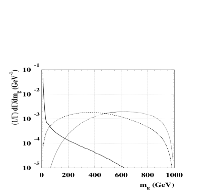
Figure 3: Mass distribution (left) and energy distribution (right) for the graviton radiated in the decay of one matter KK excitation with mass 1 TeV. Straight lines corresponds to $N=2$ extra dimensions, dashed lines to $N=4$, and dotted lines to $N=6$. The integral of the area under the individual curves is equal to 1.

Note also that the form factor associated with the decays to spin-two and scalar gravitons has a suppression effect on the cross-section, even if the masses of the final state gravitons are large (this happens because $n_{5}$ is typically much smaller than $|{\vec{n}}|$). This does not matter very much for $N=2$, because of the $(M/m_{g})^{4}$ enhancement factor. In particular, for $N=2$, since mostly the lightest gravitons contribute, one can estimate the relative decay widths to spin-two, vector and scalar gravitons from Eqs. (3.3), (3.3). One obtains $\Gamma_{h}:\Gamma_{A}:\Gamma_{\phi}\sim 1:0:1/8$ for fermions, and $\Gamma_{h}:\Gamma_{A}:\Gamma_{\phi}\sim 1:3:1/8$ for bosons (the smallness of the decay width to vector gravitons for fermions is due to the absence of the enhancement factor $(M/m_{g})^{2}$). However, for $N\geq 3$ this means that the decay width to spin-two and scalar gravitons is suppressed in comparision to the decay width to vector gravitons.

As an illustration, we plot in Fig. 3 (left panel) the partial decay width as a function of graviton mass (computed for the decay of a 1 TeV KK excitation of a fermion). One sees that the above analysis is correct, and the total decay width for $N=2$ is due mostly to light gravitons, while for $N=4,6$ heavier gravitons dominate. In the right panel, we plot the energy of the final state graviton (which has implications for the collider phenomenology of the model, as it will be discussed in the next section). Thus, for $N=2$, the graviton energy is equal to about half the mass of the particle (since for this purpose the graviton mass can be taken to be close to zero), while for higher $N$, the graviton has typically an average energy closer to three quarters of the mass $M$ of the decaying particle.

Figure 4: Decay widths for KK fermions (left) and bosons (right) as a function of the particle mass. Straight lines corresponds to $N=2$ extra dimensions, dashed lines to $N=4$, and dotted lines to $N=6$. Here $M_{D}$ is taken to be 5 TeV.

In Fig. 4 we plot the total gravitational decay widths for KK excitations of fermions (left panel) and gauge bosons (right panels). We take $M_{D}=5$ TeV, and let $M$ to vary from 200 GeV up to 3 TeV. We see that generally the decay widths are larger for $N=2$ (due to smaller mass splitting between the graviton masses, as well as due to the enhancement factor discussed above). Also, even for $N=6$, the decay widths are typically large enough that the particles will decay into detector. Moreover, among the first level KK excitations, the gravitational decay widths are comparable with the decay widths due to mass splittings. A direct comparision of the widths associated with these two types of decays can be found in Ref. (cmn2); however, one must keep in mind that the results for gravitational decays depends strongly on the parameters $M,M_{D}$, and as such, care must be used when commenting on the relative importance of the two decay modes

In order to facilitate such a comparision, we shall give here on the dependence of the gravitational decay widths on the parameters $M$ and $M_{D}$. For $N=3,\ldots,6$, the behaviour of the dominant terms (large $m$) in the integral (29) goes like $m^{N-1}M^{3}/M_{D}^{N+2}$. Since the upper limit for $m$ in the integral is $M$, this would lead to a behaviour $\Gamma_{h}\sim M^{N+3}/M_{D}^{N+2}$ (consistent with the results shown in Fig. 4). On the other hand, for $N=2$ only the gravitons with lowest masses typically give a nonnegligible contribution to the total width, and therefore $\Gamma_{h}$ scales like the decay width to the lowest mass graviton $\Gamma_{h}\sim(1/M_{pl}^{2})M^{5}/(m_{g}^{0})^{2}\sim M^{5}/M_{D}^{4}$ (where we have made use of the ADD relation (28) ). These relations can be verified by numerical computations.

3.4 Phenomenology of gravity-mediated decays

In this section we will discuss the phenomenology of models in which the decay of matter KK excitations can be mediated by gravity. In such cases, the experimental signal observed will be the SM particle(s) corresponding to the KK excitation(s) which decays gravitationally, and missing energy taken away by the gravitons (which interact too weakly to be observed in the detector). By contrast with the case where the LKP is stable, the energies of the SM particles observed (either quarks and gluons, which will appear as jets, or leptons and photons) will be large, since they are the final products of the decay of a massive particle (the KK excitation). One therefore obtains a strong signal in such scenarios, which makes it easy to observe the new particles and/or constrain the model.

Figure 5: Regions in the parameter space where decays to $\gamma^{*}$ dominate versus the gravitational decays for $q^{*},g^{*}$. The solid, dashed and dotted lines correspond to $N$ = 6, 4 and 2 extra dimensions.

Depending on the relative strength of the decay channels of the KK excitations, one can identify three separate scenarios for the phenomenological signal. First is the case when the gravitational decays dominate. Then, KK excitations of quarks and gluons decay to SM quark and gluons plus gravitons. The experimental signal in this case will be jets plus missing energy. Second, one can have the case when the decays due to mass splitting between the first level KK excitations take place first. Then, the KK excitations of quarks and gluons will decay to the LKP (the $\gamma^{*}$), radiating low $p_{T}$ quarks and leptons in the process; the LKP will then decay gravitationally, leaving behind high $p_{T}$ photons and gravitons (which will appear as missing energy). Finally, one can have the intermediate case, when the gravitational and strong/electroweak decay widths are of comparable magnitude. Then it is possible for a $q^{*}$ to follow just several steps in the decay chains (2.3.1), for example to a $l^{*}$, and the KK exictation of the lepton to decay gravitationally, leaving behind a high $p_{T}$ lepton.

Which one of this scenarios will happen in practice depends on the parameters of the model. One can easily imagine situations in which either case happens. For example, if $N=2$, $M_{D}$ is small, and/or the mass of the KK excitations is somewhat large, the gravitational decay widths will tend to dominate. On the other hand, if $N=6$, $M_{D}$ is large, and/or the masses of KK excitations are relatively light, the strsong/electroweak decays to the LKP will take place first. For illustration, we present in Fig. 5 the contour lines in the $(M_{D},M)$ plane for which the KK fermion gravitational decay width is equal to the $l^{*}\rightarrow l\gamma^{*}$ decay width (evaluated for $\Lambda R=20$ ). This means that for values of $M_{D},M$ which fall bellow the lines in the plot, the decay to $\gamma^{*}$ happens first. For points which are right on the lines (or close to them), typically partial decays to $Z^{*}$ or $l^{*}$ happen, followed by the gravitational decays of these excitations. For points significantly above the lines (of order 100 GeV in $M$), the quark or gluon excitations decay directly to gravitons and the SM partners.

Figure 6: The cross-section for dijet + missing energy production as a function of KK excitations mass for Tevatron Run II (left panel) and LHC (right panel). The solid lines correspond to $N=2$ extra dimensions, and the dashed lines to $N=6$. The kinematic cuts applied are described in the text.

We will start by discussing the phenomenology of first type scenarios (with gravitational decay widths dominant). This has been studied in some detail in Ref. (cmn); here we will review the results. The mechanism through which KK excitations are produced is the pair production processes discussed in section 2.2. The observable signal will be two jets plus missing energy. The cross sections for this signal (with a $p_{T}$ cut on the jet transverse momentum) are shown in Fig. 6 as a function of the mass of quark KK excitations $m_{KK}$ (as shown in Figs 1, 2, the final state contains mostly $q^{*}$). The left panel corresponds to the Tevatron Run II case (with $p_{T}>100$ GeV), while the right panel corresponds to the LHC case (with $p_{T}>600$ GeV). Additional cuts are applied on the rapidity of the individual jets $|y|<2.5$, and the angular separation between the two jets $R=\sqrt{\Delta\phi^{2}+\Delta\eta^{2}}>0.4$.

The reason for applying such high $p_{T}$ cuts is to help eliminate the Standard Model backgrounds. Such backgrounds will be due to the production of the $Z$ gauge boson with two jets (where $Z$ decays to $\nu\bar{\nu}$ or $\tau\bar{\tau}$ pairs), W + 2 jets (with the lepton from the W decay unidentifiable), $t\bar{t}$ production, with one top decaying semileptonically to $b\bar{\nu}l$ with the lepton unidentified, and to QCD multijet production with mismeasured missing energy ($\not{E_{T}}$). It is also desirable to impose an $\not{E_{T}}$ cut on our signal. Since the jets we observe in our model result from the decay of heavy particles (the KK excitations), they are likely to have a large $p_{T}$. Also, since the gravitons have large momentum, the missing energy is likely to be large, too. At large $p_{T},\not{E_{T}}$ cuts, the dominant SM background process will come from the $Z$ + 2 jets production, and this falls rapidly with increasing $p_{T},\not{E_{T}}$ (see, for example, Refs. (Bityukov,tata_lhc,Gaines)). It was shown in Ref. (cmn) that it typically possible to separate the signal from the background by using cuts of the type $p_{T}>p_{T}^{0},\not{E_{T}}>2p_{T}^{0}$, where values for $p_{T}^{0}$ can be chosen such as to maximize the significance, defined as the signal divided by the square root of the background.

Another interesting issue is how could one measure the mass of KK excitations and the number of extra dimensions $N$ if such signals are observed. Of course, the magnitude of the cross section will give a first order approximation for the mass of the KK excitations. However, as it can be seen in Fig. 6, the observable cross section also has a somewhat weaker dependence on $N$. Additional information about the $M,N$ parameters can be obtained by looking at the dependence of the signal cross-section on the $p_{T}$ cut, and also on the missing energy. As shown in Ref. (cmn), the cross section decreases faster as a function of $p_{T}$ cut for more extra dimensions; also the missing energy is typically smaller. The reason for this behavior is that the larger the number of extra dimensions, the higher is the mass of the gravitons which are radiated in the decay of the KK excitations (as discussed in the previous section); therefore, the smaller the energy available for the SM quarks or gluons. Analysis of such distributions could then provide sufficient information to infer the value of the mass $M$ precisely, as well as the number of extra dimensions.

Finally, one should consider ways to differentiate between different theories which give rise to similar signals. One other obvious candidate is supersymmetry, in which case jets + missing energy signal would arise from gluinos (or squarks) which decay to a quark antiquark pair (or a single quark) and a neutralino LSP (lightest supersymmetric particle). Then one would see jets in the detector generated by these quarks, which have generally a large energy/transverse momentum (since the mass splitting betwen the squarks and the LSP is typically large), while the LSP, which is stable, will show as missing energy (playing the role of the graviton). An analysis aiming to discriminate between the signatures of UED/supersymmetry by using the kinematic features of the observable jets is underway[50].

We turn now to the analysis of the case when the decay modes allowed by mass splitting among the first level KK excitations are dominant (this can happen for large value of the fundamental scale $M_{D}$, for example). In this scenario, as discussed in Ref. (cmn2), the KK excitations of quarks and gluons pair-produced at a hadron collider will first decay to the LKP (the $\gamma^{*}$), radiating low $p_{T}$ quaks and leptons in the process; the LKP will then decay gravitationally. The signal for such a case will then be two high $p_{T}$ photons, accompanied by several jets and leptons with low $p_{T}$, and large missing energy.

Figure 7: The cross-section for diphoton + missing energy production as a function of $1/R$ for Tevatron Run II (left panel) and LHC (right panel). The solid lines correspond to $N=2$ extra dimensions, and the dashed lines to $N=6$. The kinematic cuts applied are described in the text.

The Standard Model background for this signal is very small; the most important component arise from misidentification of jets or leptons as photons, and/or mismeasured $\not{E_{T}}$. Hence, one does not need to impose such high $p_{T}$ cuts on the momenta of the observable photons. In Fig. 7 we show the cross section for this signal at the Tevatron Run II (left panel) and LHC (right panel), with the following cuts: $p_{T}>20$ GeV, $\not{E_{T}}>50$ GeV for Tevatron, and $p_{T}>200$ GeV, $\not{E_{T}}>200$ GeV for the LHC. The estimated backgrounds with these cuts are 0.5 fb at the Tevatron[52], and 0.05 fb at the LHC[53]. Note that these plots are shown as a function of the thickness of the brane $1/R$, and that the masses of the KK excitations are somewhat different from this due to radiative corrections.

Such signals can also arise in different theories, for example in a supersymmetric model with gauge mediated SUSY breaking. In such a case, the LSP is the goldstino/gravitino, which is esentially massless[54]. The next-to-lightest supersymmetric particle (NLSP) may very well be a (bino-like) neutralino, which will decay to the goldstino with the radiation of a photon. Then the squarks and gluinos predominatly produced at a hadron collider will decay first to the NLSP (while radiating jets and leptons which may be hard or soft, depending on the mass splittings and the parameters of the model), and this in turn will decay to a hard $p_{T}$ photon and an invisible goldstino (missing energy). The signal in this case may be very similar to the one discussed for the UED model in which the KK excitations decay first to the LKP, and an analysis to try to differentiate these two scenario needs to be done.

Finally, we shall make some comments on the case when the decay widths due to gravitational interactions and the decay widths due to mass splitting are of the same order of magnitude. Then, one of the KK excitations of quarks and gluons can decay gravitationally, while the other may decay first to the LKP. The signal in this case would be jet+ photon + missing energy. It is also possible that one (or both) of the initial KK excitations will decay to a KK excitation of a lepton, which in turn will decay gravitationally, leading to signals with jet+lepton, photon + lepton and two leptons in the final state.

Figure 8: Branching ratios to final states: $\gamma\gamma$ (solid line), jet + $\gamma$ (dotted line) and lepton ($e$ or $\mu$) + $\gamma$ (dashed line) for $M_{D}=5$ TeV and $\Lambda R=20$, at the Tevatron Run II and $N=2$(left), and LHC and $N=6$ (right). (Redo the figure)

The relevant fact to keep in mind when discussing this case is that what will happen is strongly dependent on the parameters of the model. Unlike the two previously discussed cases, where the type of signal (as well as its magnitude) is more or less independend of parameters like $M_{D}$ or $\Lambda$ (as long as we are in a situation when one or the other of the decay modes dominates), when the decay widths are of the same order of magnitude, the type of signal is strongly dependent on $M_{D},\Lambda$ as well as $1/R$. For an example of such a situation, one can look at the case when $M_{D}=5$ TeV, $\Lambda R=20$; as can be seen in Fig. 3 in Ref. (cmn2), the decay widths are of the same order of magnitude for N=2 and small values of $1/R$ (of order 500 GeV), or, conversely, for $N=6$ and larger values of $1/R$ (of order 3 TeV). Then, as illustrated in Fig. 8, the type of signal one sees depends on the value of $1/R$. Moreover, there are regions in the parameter space where one will see different signals, if the branching ratios for decays leading to different final states are of the same order of magnitude.

3.5 Single KK excitation production

We turn now to a discussion of the consequences which the introduction of a KK number violating gravitational interaction has on the production of matter KK excitations at colliders. Such interaction gives rise to processes with only one KK particle in the final state. KK gravitons may appear either as intermediate (virtual) particles mediating the production of a SM quark/gluon and one KK excitation, or as real particles in the final state. Since the minimum center-of-mass energy required for such processes is lower than for the case of KK pair production, one can probe higher values for $m_{KK}$ in this channel. However, since the gravitational interaction is involved in production, one also typically needs a low value for the fundamental gravity scale parameter $M_{D}$.

3.5.1 Gravity-mediated production

We discuss in this section the production of a single KK excitation of matter (quark or gluon) mediated by virtual gravitons. The Feynman diagrams of the processes contributing to this signal are of the type shown in Fig. 9 (processes with gluons or $q\bar{q}$ quark pairs in the initial and final state also have an $s$-channel contribution). The list of all the processes with final state $q^{*}$’s or $g^{*}$’s can be found in Ref. (marius1), together with the corresponding amplitudes.

Figure 9: Feynman diagrams ($t$ and $u$ channel) contributing to the production of a $qq^{*}$ final state. The thick lines denotes the $q^{*}$ excitation, while the double helix ones denotes the exchanged graviton.

Let us comment briefly on the graviton propagator. A single graviton couples to matter with a strength of order $E/M_{Pl}$ (where $E$ is the energy scale of the process under consideration). Therefore the contribution given by a single graviton to a process as in Fig. 9 is negligible. However, as is usual in an extra-dimensional scenario, there is an entire tower of gravitons $h_{{\vec{n}}}$ which may contribute, and when one sums the amplitudes coming from the individual excitations, one obtains a sizable contribution.

In the evaluation of the amplitudes for the processes of interest to us, one therefore uses a resummed graviton propagator

$$D_{\mu\nu,\rho\sigma}(k^{2})\ =\ \sum_{\vec{n}}D_{\mu\nu,\rho\sigma}^{\vec{n}}(k^{2})\ =\ \kappa^{2}\ \sum_{\vec{n}}{\cal F}_{00|n_{5}}\ {iB_{\mu\nu,\rho\sigma}(k)\over s-m_{\vec{n}}^{2}}\ ({\cal F}^{c}_{10|n_{5}})^{*}\ ,$$ (30)

where $B_{\mu\nu,\rho\sigma}(k)$ is the denominator of the propagator for a massive spin-two particle (see, for example, Ref. (HLZ)), and ${\cal F}_{00|n_{5}}$ and ${\cal F}^{c}_{10|n_{5}}$ are form factors describing the interaction of the gravitons with the matter excitations on the brane (see section 3.2). The ‘$00$’ and ‘$10$’ indices show that the graviton couples to two Standard Model particles at one end, and to one SM particle and its first level KK excitation at the other end. Terms $\sim k^{\mu}T^{0}_{\mu\nu}$, where $T^{0}_{\mu\nu}$ is the energy-momentum tensor associated with Standard Model matter are zero; hence the resummed graviton propagator will have the form

$$D(k)_{\mu\nu,\rho\sigma}=\left(\eta_{\mu\rho}\eta_{\nu\sigma}+\eta_{\mu\sigma}\eta_{\nu\rho}-{2\over 3}\eta_{\mu\nu}\eta_{\rho\sigma}\right)D(k^{2})\ .$$

The function $D(k^{2})$ can be evaluated by replacing the sum in Eq. (30) by an integral (as described in section 3.3). Generally, this integral has to be performed numerically; however, in the limit where $k^{2},M$ are much smaller than the maximum mass of the gravitons, one can obtain the approximate expression[46] (valid for $N>3$):

$$D(k^{2})\ \simeq\ V_{N-1}\ {32\over N-3}{M\ M_{S}^{N-3}\over M_{D}^{N+2}}{2\sqrt{2}\over\pi^{2}}\ \int_{0}^{\pi M_{s}/M}{\sin x\over 1-x^{2}/\pi^{2}}dx\ ,$$ (31)

where $M=1/R$, and $V_{N-1}$ is the area of a sphere in $N-1$ dimensions (due to the form factor, the integrand is not symmetric under rotations in $N$ dimensions, but rather in $N-1$ dimensions).

The quantity $M_{S}$ in the above expression stands for the upper limit on the graviton masses. Note that the sum (30) is not convergent for $N>2$; one therefore has to impose a cut-off on the massive graviton contributions. The scale of the cut-off is typically taken to be the same as the fundamental gravity scale: $M_{S}\sim M_{D}$; the reason for this being that the scattering amplitudes we compute are valid in the low energy limit $E\ll M_{D}$. Once we get close to the gravity scale, our perturbative field-theory description is quite possible not valid anymore, and one may have to employ alternative descriptions, like string theory/black hole scattering[55, 56]. Different choices for $M_{S}$ can then be thought of as parametrization of this new physics. In our following discussion, we will take $M_{S}=M_{D}$, but one should keep in mind that for this type of process, for $N>3$ the magnitude of the cross section varies with $M_{S}$ (like $M_{S}^{2(N-3)}$, in fact), and the computed signal can easily be larger or smaller depending upon this choice.

The observable signal for such a process will be two jets plus missing energy (assuming that the gravitational decay width dominates). This is similar to the case of KK pair production; however, the jets are asymmetric in this case (since only one arises from the decay of a heavy KK particle, while the other is produced directly). Typically, the jet coming from the decay of the KK particle has higher $p_{T}$ (depending on the mass of the excitation), and it should be possible to differentiate between the two. Also, due to the fact that only one massive particle is in the final state, it should be possible to probe higher values of $1/R$ than in the pair production case. This is however, dependent upon the condition that the fundamental gravity scale is low enough; since the cross-section behaves like $1/M_{D}^{10}$, increasing $M_{D}$ will rapidly make the signal unobservable.

Figure 10: Tevatron and LHC reach for 10 and 50 signal events (at the Tevatron), and 20 and 100 signal events (at the LHC). Straight and dotted lines corresponds to $N=6$, and dashed and dotdashed line correspond to $N=2$, respectively. The cuts are described in the text.

For illustration, we show in Fig. 10 the Tevatron and LHC reach as a function of $(M_{D},M=1/R)$. At Tevatron, the straight and dashed lines correspond to a cross-section of 10 fb (with $N=2$ and $N=6$, respectively), and dotted and dash-dotted lines correspond to a cross-section of 50 fb (for $N=2$ and $N=6$). The cuts used are $p_{T}>150$Gev for both jets, and $\not{E_{T}}>$ 300 GeV. The background is the same as the one discussed for the pair production case, and with an integrated luminosity of 2 fb^-1, it amounts to one event (the signal being then 10 and 50 events). We see that for relatively low values of $M_{D}$, one is able to almost double the $m_{KK}$ discovery reach, from four to five hundred GeV at the Tevatron (Fig 6), to almost 800 GeV.

The right panel in Fig. 10 shows the LHC reach. The straight and dashed lines correspond to a cross-section of 0.2 fb (with $N=2$ and $N=6$, respectively), and dotted and dash-dotted lines correspond to a cross-section of 1 fb (for $N=2$ and $N=6$). The cuts used are $p_{T}>800$ Gev for both jets, and $\not{E_{T}}>$ 1.6 TeV. The background with these cuts (and 100 fb^-1 integrated luminosity) is around 10 events, while the signal will be 20, respectively 100 events. The discovery reach for low values of $M_{D}$ also increases in this case compared to the pair production case.

This type of signals have been studied in Ref. (marius1). However, one can also have $ll^{*}$ and $\gamma\gamma^{*}$ final states, from processes with the exchange of $s$ channel gravitons. This requires that the initial state is either $q\bar{q}$ or $gg$, therefore the production cross section will be somewhat smaller than for the case of quarks of gluons in the final state. However, the observable signal will be two high $p_{T}$ photons or leptons, and the SM background will be much reduced. Detailed simulations have not been performed yet, but one would expect that the discovery reach in this channel will be as large as in the two jets case, or even larger.

Finally, it is interesting to consider that in searching for universal extra dimensions, one can look at KK pair production and gravity mediated single KK production as somewhat complementary channels. If $M_{D}$ is relatively small, the pair produced KK excitations will decay to jets + gravitons, thus making them somewhat hard to see at hadron colliders; however, in this case the cross section for single KK production can be quite large. On the other hand, if the gravity scale is larger, the cross-section for the production of a single KK excitation will be small; but then the pair-produced KK excitations will decay first to $\gamma^{*}$, and the two photons + large $\not{E_{T}}$ signal will make the signal in this channel easier to see at hadron colliders.

3.5.2 Final state gravitons

We end our review of the phenomenology of universal extra dimensions with a short discussion of the case when a single KK excitation of matter is produced with a graviton KK excitation in the final state. Again, the production rate for a particular graviton excitation is small (of order $E/M_{Pl}$), but when summing over the KK tower one can obtain a sizable cross-section.

The amplitudes contributing to the processes of interest here are the same ones encountered in the evaluation of the production rate for a Standard Model particle plus a KK graviton in the usual ADD model[39, 42]. Indeed, where one produces the KK excitation of a quark or gluon, one can also produce the Standard Model particle together with the graviton. If the KK quark or gluon decays to a jet, one obtains the same type of signal (jet plus missing energy) in both cases. Since the process with the SM particle in the final state is phase-space favored (no need to produce a massive excitation), one can conclude that the production of a KK excitation of matter is at most a small correction.

However, a more detailed analysis is needed to support this conclusion. As discussed above, high $p_{T}$ and missing energy cuts (of order of TeV at the LHC) might be needed to separate the signal in this case from the SM background. Since the jet coming from the decay of a heavy KK excitation will typically have a higher transverse momentum than a jet coming from a directly produced quark or gluon, it is possible that in the region of phase space of interest experimentally the signals for the two types of processes are of comparable orders of magnitude. Moreover, if one sees just an excess of jets with missing energy at a hadron collider, while it is possible to infer the existence of new physics, it will not be clear what type of physics it is. For example, besides the fat brane scenario we discuss here, it could be supersymmetry, or a pure ADD model (with matter restricted on the 4D brane). An analysis of relevant phenomenological observables (like $p_{T}$ distributions) will be needed to determine the exact theory.

The signal for this case has been studied in Ref. (Marius2). Results indicate that the cross-section for the production of gravitons + KK excitations of matter is indeed significantly smaller than the cross section for the production of gravitons + SM matter. The phase space constraints play a role, but additionally this is due in part to the effect of the form-factor. As discussed in section 3.2, the interaction vertex of matter with gravity aquires a form factor ${\cal F}^{c}_{1|n_{5}}(x)$, $x=2\pi n_{5}R/(lr)$, proportional to the superposition of wave functions of matter and gravity in the fifth direction (see Eq. (26)). Since $|{\cal F}^{c}_{1|n_{5}}(x)|^{2}\sim x^{2}$ for small $x$, this has as result a suppression of the production cross section.

As a consequence, it will be quite hard to see the production of a matter KK excitation with a graviton in the jet plus missing energy channel. However, a better chance for the observation of this process happens for the case when the mass-splitting decay modes dominate, and the gluon or quark excitation decays first to $\gamma^{*}$. The background for the signal in this case (high energy photon with missing transverse energy) is low in the Standard Model, as well as in the case of production of KK gravitons with a SM photon (since the strength of the interaction is governed by the electroweak coupling), and it is possible to measure a small signal cross-section. Moreover, for small values of $N$, the production cross section decreases slower with $M_{D}$ than for the case of gravity-mediated single KK production ($\sigma\sim 1/M_{D}^{N+2}$ versus $1/M_{D}^{10}$ in the later case), so one can potentially probe larger values of $M_{D}$. Thus, if the mass of the matter KK excitations is not too big (of order 1 TeV or smaller), for $N=2$ it might be possible to probe values for $M_{D}$ as large as 40 TeV.

4 Conclusions

Theoretical considerations (like string theory) suggest that there may be more than 4 space-time dimensions. If the compactification scale for the extra dimensions is relatively large, they may be the of relevance for low energy physics. In particular, models where matter propagates in extra dimensions of inverse TeV scales have interesting implications for the phenomenology of present-day and future colliders. We review in this article the collider phenomenology associated with a particular class of models, Universal Extra Dimensions, in which all matter fields propagate in the bulk.

A characteristic feature of such theories is Kaluza Klein parity conservation, which requires that the KK excitations of Standard Model particles are produced in pairs. Moreover, the lightest KK particle (LKP) is stable, and generally weakly interacting. The masses of the first level excitations aquire radiative corrections, with strongly interacting particles getting higher masses than the excitations of leptons and weakly interacting bosons. Therefore, first KK level quarks and gluons produced at a hadron collider will decay to the LKP, radiating semi-soft leptons and jets. Experimental signals for this scenario will be similar to that of a supersymmetric model with almost degenerate mass spectrum for the superpartners, and the lightest supersymmetric particle (LSP) being a neutralino.

Adding gravitational interactions will modify somewhat this picture. Such interactions might break KK number conservation, since gravity and matter do not have to propagate on the same scale in the extra dimensions. In fact, there are theoretical arguments supporting the view that gravity should propagate in ’large’ extra dimensions with inverse eV size, while matter fields should be stuck close to the 4D brane, with only a length $\sim 1/M_{D}\sim$ TeV^-1 accesible to them (the fat brane scenario). Then the KK excitations of matter (including the LKP) can decay to SM particles and KK gravitons.

The phenomenology resulting from KK pair production will be then quite different. Generally speaking, there will be two high $p_{T}$ particles/jets in the final state, corresponding to the decay of the KK excitations, and missing energy associated with gravitons. The exact nature of the final state particles depends on the details of the model; thus, if gravitational decays widths are large, the KK excitations of quarks and gluons produced at a hadron collider will decay directly to SM quarks and gluons, which will appear as jets in the detector. However, if the gravitational decays widths are small, the KK quarks and gluons will first decay to the LKP (radiating soft jets and leptons in the process) which then will decay gravitationally, leading to a signal with two high $p_{T}$ photons in the final state. If the two decay modes are of comparable importance, one can obtain a mix-up of final state high $p_{T}$ particles, including photons, jets and leptons.

Moreover, in this scenario it is possible to produce a single KK excitation of matter through processes involving gravitons. Since the effective strength of the gravitational interaction is $\sim 1/M_{D}^{2}$, this requires that the fundamental gravity scale $M_{D}$ be rather low. However, since one need to produce only one massive particle in the final state, one can probe higher values for the masses of matter KK excitations in this type of process.

The experimental signals for such production processes can also be two jets, photons or leptons, jet and photon or lepton, single jet or single photon with missing energy in the final state. Such signals can arise in a variety of supersymmetric models too; for example, final states with jets and/or leptons can arise in MSUGRA models with squarks and gluinos decaying to a significantly lighter LSP neutralino (cascade decays through charginos might account for the leptons). Final states with high $p_{T}$ photons can arise in gauge mediated supersymmetry breaking (GWSB) models, where the LSP is a very light goldstino/gravitino. In conclusion, this class of models leads to a rich phenomenlogy, and a careful study is needed to discriminate between SUSY and UED signals at hadron colliders.

References

- [1] L. Randall and R. Sundrum, Phys. Rev. Lett. 83, 3370 (1999) and Phys. Rev. Lett. 83, 4690 (1999).
- [2] N. Arkani-Hamed, S. Dimopoulos and G. Dvali, Phys. Lett. B429, 263 (1998) and Phys. Rev. D59, 086004 (1999);I. Antoniadis, N. Arkani-Hamed, S. Dimopoulos and G. Dvali, Phys. Lett. B436, 257 (1998); I. Antoniadis, Phys. Lett. B246, 377 (1990).
- [3] E. Accomando, I. Antoniadis and K. Benakli, Nucl. Phys. B 579, 3 (2000) [arXiv:hep-ph/9912287].
- [4] P. Nath, Y. Yamada and M. Yamaguchi, Phys. Lett. B 466, 100 (1999) [arXiv:hep-ph/9905415].
- [5] D. A. Dicus, C. D. McMullen and S. Nandi, Phys. Rev. D 65, 076007 (2002) [arXiv:hep-ph/0012259].
- [6] T. G. Rizzo, Phys. Rev. D 61, 055005 (2000) [arXiv:hep-ph/9909232].
- [7] M. Masip and A. Pomarol, Phys. Rev. D 60, 096005 (1999) [arXiv:hep-ph/9902467].
- [8] T. G. Rizzo and J. D. Wells, Phys. Rev. D 61, 016007 (2000) [arXiv:hep-ph/9906234].
- [9] P. Nath and M. Yamaguchi, Phys. Rev. D 60, 116004 (1999) [arXiv:hep-ph/9902323].
- [10] T. Appelquist, H. C. Cheng and B. A. Dobrescu, Phys. Rev. D 64, 035002 (2001) [arXiv:hep-ph/0012100].
- [11] T. G. Rizzo, Phys. Rev. D 64, 095010 (2001) [arXiv:hep-ph/0106336].
- [12] C. Macesanu, C.D. McMullen and S. Nandi, Phys. Rev. D66, 015009 (2002).
- [13] K. Agashe, N. G. Deshpande and G. H. Wu, Phys. Lett. B 514, 309 (2001) [arXiv:hep-ph/0105084].
- [14] T. Appelquist and B. A. Dobrescu, Phys. Lett. B 516, 85 (2001) [arXiv:hep-ph/0106140].
- [15] T. Flacke, D. Hooper and J. March-Russell, arXiv:hep-ph/0509352.
- [16] H. C. Cheng, K. T. Matchev and M. Schmaltz, Phys. Rev. D 66, 056006 (2002) [arXiv:hep-ph/0205314].
- [17] H. C. Cheng, K. T. Matchev and M. Schmaltz, Phys. Rev. D 66, 036005 (2002) [arXiv:hep-ph/0204342].
- [18] G. Servant and T. M. P. Tait, Nucl. Phys. B 650, 391 (2003) [arXiv:hep-ph/0206071].
- [19] H. C. Cheng, J. L. Feng and K. T. Matchev, Phys. Rev. Lett. 89, 211301 (2002) [arXiv:hep-ph/0207125].
- [20] A. De Rujula, A. Donini, M. B. Gavela and S. Rigolin, Phys. Lett. B 482, 195 (2000) [arXiv:hep-ph/0001335].
- [21] C. Macesanu, C.D. McMullen and S. Nandi, Phys. Lett. B546, 253 (2002).
- [22] B. A. Dobrescu and E. Poppitz, Phys. Rev. Lett. 87, 031801 (2001) [arXiv:hep-ph/0102010].
- [23] T. Appelquist, B. A. Dobrescu, E. Ponton and H. U. Yee, Phys. Rev. Lett. 87, 181802 (2001) [arXiv:hep-ph/0107056].
- [24] G. Burdman, B. A. Dobrescu and E. Ponton, arXiv:hep-ph/0506334.
- [25] K. R. Dienes, E. Dudas and T. Gherghetta, Nucl. Phys. B 537, 47 (1999) [arXiv:hep-ph/9806292].
- [26] J. Papavassiliou and A. Santamaria, Phys. Rev. D 63, 125014 (2001) [arXiv:hep-ph/0102019].
- [27] A. Connolly [CDF collaboration], ”Search for long-lived charged massive particles at CDF,” Talk at the American Physical Society (APS) Meeting of the Division of Particles and Fields (DPF ), Los Angeles, CA, Jan -, , arXiv:hep-ex/9904010.
- [28] H. Georgi, A. K. Grant and G. Hailu, Phys. Lett. B 506, 207 (2001) [arXiv:hep-ph/0012379].
- [29] R. Sekhar Chivukula, D. A. Dicus and H. J. He, Phys. Lett. B 525, 175 (2002) [arXiv:hep-ph/0111016].
- [30] S. M. Wang, “ Searches for Higgs and New Phenomena at CDF ”.
- [31] S. Abel et al. [SUGRA Working Group Collaboration], arXiv:hep-ph/0003154.
- [32] H. Baer, C. h. Chen, F. Paige and X. Tata, Phys. Rev. D 53, 6241 (1996) [arXiv:hep-ph/9512383].
- [33] A. J. Barr, Phys. Lett. B 596, 205 (2004) [arXiv:hep-ph/0405052].
- [34] A. Datta, K. Kong and K. T. Matchev, arXiv:hep-ph/0509246.
- [35] J. M. Smillie and B. R. Webber, arXiv:hep-ph/0507170.
- [36] M. Battaglia, A. Datta, A. De Roeck, K. Kong and K. T. Matchev, JHEP 0507, 033 (2005) [arXiv:hep-ph/0502041].
- [37] G. Bhattacharyya, P. Dey, A. Kundu and A. Raychaudhuri, arXiv:hep-ph/0502031.
- [38] J. Lykken and S. Nandi, Phys. Lett. B 485, 224 (2000), [arXiv:hep-ph/9908505].
- [39] E. A. Mirabelli, M. Perelstein and M. E. Peskin, Phys. Rev. Lett. 82, 2236 (1999) [arXiv:hep-ph/9811337].
- [40] J. L. Hewett, Phys. Rev. Lett. 82, 4765 (1999) [arXiv:hep-ph/9811356].
- [41] T. Han, J.D. Lykken and R.-J. Zhang, Phys. Rev. D59, 105006 (1999).
- [42] G. F. Giudice, R. Rattazzi and J. D. Wells, Nucl. Phys. B 544, 3 (1999) [arXiv:hep-ph/9811291].
- [43] A. De Rujula, A. Donini, M. B. Gavela and S. Rigolin, Phys. Lett. B 482, 195 (2000) [arXiv:hep-ph/0001335].
- [44] C. Macesanu, S. Nandi and M. Rujoiu, Phys. Rev. D 71, 036003 (2005) [arXiv:hep-ph/0407253].
- [45] C. Macesanu, S. Nandi and M. Rujoiu, arXiv:hep-ph/0510350.
- [46] C. Macesanu, A. Mitov and S. Nandi, Phys. Rev. D 68, 084008 (2003) [arXiv:hep-ph/0305029].
- [47] J. L. Feng, A. Rajaraman and F. Takayama, Phys. Rev. D 68, 085018 (2003) [arXiv:hep-ph/0307375].
- [48] S. I. Bityukov and N. V. Krasnikov, Phys. Lett. B 469, 149 (1999) [Phys. Atom. Nucl. 64, 1315 (2001 YAFIA,64,1391-1398.2001)] [arXiv:hep-ph/9907257].
- [49] H. Baer, C. h. Chen, F. Paige and X. Tata, Phys. Rev. D 52, 2746 (1995) [arXiv:hep-ph/9503271].
- [50] C. Macesanu, S. Nandi and M. Rujoiu, in preparation
- [51] I. Gaines, D. Green, S. Kunori, S. Lammel, J. Marraffino, J. Womersley and W. Wu, FERMILAB-FN-0642.
- [52] R. Culbertson et al., “Low-scale and gauge-mediated supersymmetry breaking at the Fermilab Tevatron Run II,” arXiv:hep-ph/0008070.
- [53] H. Baer, P.G. Mercadante, F. Paige, X. Tata and Y. Wang, Phys. Lett. B435 109 (1998).
- [54] S. Dimopoulos, M. Dine, S. Raby and S. Thomas, Phys. Rev. Lett. 76, 3494 (1996) [arXiv:hep-ph/9601367].
- [55] S. Cullen, M. Perelstein and M. E. Peskin, Phys. Rev. D 62, 055012 (2000) [arXiv:hep-ph/0001166].
- [56] M. Cavaglia, Int. J. Mod. Phys. A 18, 1843 (2003) [arXiv:hep-ph/0210296].