MULTI-PARTICLE PROCESSES IN THE STANDARD

MODEL WITHOUT FEYNMAN DIAGRAMS  

Abstract

A method to efficiently compute, in a automatic way, helicity amplitudes for arbitrary scattering processes at leading order in the Standard Model is presented. The scattering amplitude is evaluated recursively through a set of Dyson-Schwinger equations. The computational cost of this algorithm grows asymptotically as $3^{n}$, where $n$ is the number of particles involved in the process, compared to $n!$ in the traditional Feynman graphs approach. Unitary gauge is used and mass effects are available as well. Additionally, the color and helicity structures are appropriately transformed so the usual summation is replaced by Monte Carlo techniques. Some results related to the production of vector bosons and the Higgs boson in association with jets are also presented.

1 Introduction

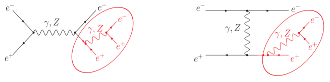
Figure 1: An example of common parts of the amplitudes (in red) for the $e^{+}e^{-}\rightarrow e^{+}e^{-}e^{+}e^{-}$ process.

Multi-particle and multi-jet final states are of great importance at the TeVatron and at the future LHC or $e^{+}e^{-}$ Linear Collider. They serve both as signals and as important backgrounds to many new and already discovered physics channels. As an example the production and decay of top quarks, Higgs boson(s) or SUSY particles can be mentioned. A typical background is the production of weak vector bosons in association with jets. Among others the proper evaluation of the eight jet QCD background will be needed. To describe the production process of a number of particles the corresponding amplitudes have to be constructed. This usually results in a very large number of terms, such that their automated construction and evaluation becomes the only solution. Apart from handling the number of amplitudes, which grows factorially with the number of particles, the integration over the multidimensional phase space of the final state particles represents a formidable task. In the past years various solutions to deal with these problems, implemented as different codes, have been presented. Either they are based on traditional methods of constructing Feynman diagrams or alternative methods with recursive equations are implemented [1, 2, 3, 4, 5, 6, 7, 8, 9, 10, 11, 12, 13]. The new formalism based on the Dyson-Schwinger equations recursively defines one-particle off-shell Green function. It does not involve any calculation of individual diagrams but various off-shell subamplitudes are regroupped in such a way that as little of the computation as possible is repeated. On the contrary, in the traditional approach, the same parts of different Feynman diagrams are recalculated all over again, see Fig.1, increasing the number of steps that should be done in order to get the full amplitude. The recursive approach significantly decreases the factorial growth of the number of terms to be calculated with the number of particles down to $4^{n}$ or $3^{n}$ .

Some examples of automatic parton level generators for any processes in the Standard Model are CompHEP [14, 15, 16], MadGraph/MadEvent[17, 18], AMEGIC++ [19] and the HELAC/PHEGAS package [20, 21]. Codes designed for specific processes are GRACE [22, 23] as well as Alpgen [24]. Very recently also on shell recursive equations have been proposed [25, 26]. However, event generators based on this new method are not publicly available yet.

In this article the algorithm based on Dyson-Schwinger recursive equations is briefly reviewed. It has been implemented as a new version of the multipurpose Monte Carlo generator HELAC in order to efficiently obtain cross sections for arbitrary multi-particle and multi-jet processes in the Standard Model.

2 Dyson-Schwinger Recursive Equations

Dyson-Schwinger equations give recursively the $n-$point Green’s functions in terms of the $1-$, $2-$,$\ldots$, $(n-1)-$point functions. These equations hold all the information for the fields and their interactions for any number of external legs and to all orders in perturbation theory. The recursive content of the Dyson-Schwinger equations for QCD has already been introduced in Ref.[13] and reviewed recently in Ref.[27]. To include the electroweak sector, new vertices for leptons, the vector gauge bosons as well as for the scalar Higgs boson must be included. Additionally, the recursive equation for (anti)quarks should be rewritten to express their interaction with the electroweak gauge bosons.

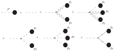
Figure 2: Recursion equations for the Higgs boson.

In order to better illustrate this idea let us present as an example the recursive equations for the Higgs boson interaction with massive particles only. Let $p_{1},p_{2},\ldots,p_{n}$ represent the external momenta involved in the scattering processs taken to be incoming. For a vector field we define a four vector $b^{\textnormal{\tiny V}}_{\mu}(P)$, which describes any sub-amplitudes from which a vector boson $V$ with momentum $P$ can be constructed. The momentum $P$ is given as a sum of external particles momenta. Accordingly we define a four-dimensional spinor $\psi^{\textnormal{\tiny F}}(P)$, which describes any sub-amplitude from which a fermion with momentum P can be constructed and by $\bar{\psi}^{\textnormal{\tiny F}}(P)$ a four-dimensional antispinor. Additionaly we have to introduces a scalar $H(P)$ for a Higgs boson. The content of Dyson-Schwinger equations in this case can be understood diagrammatically as in Fig.2. The subamplitude with an off-shell Higgs boson momentum $P$ has contributions from three-bosons and four-bosons vertices plus the fermion antifermion vertex. The black blobs denote subamplitudes with the same structure. The following general recursive equations can be written down for a Higgs boson with the momentum $P$:

$$H(P) =\sum_{i=1}^{n}\delta(P-p_{i})H(p_{i})$$

$$+\sum_{P=p_{1}+p_{2}}ig_{\textnormal{\tiny HVV}}~{}\Pi_{\textnormal{\tiny H}}~{}b^{\textnormal{\tiny V}}_{\mu}(p_{1})b^{{\textnormal{\tiny V}}\mu}(p_{2})\epsilon(p_{1},p_{2})$$

$$+\sum_{P=p_{1}+p_{2}+p_{3}}ig_{\textnormal{\tiny HHVV}}~{}\Pi_{\textnormal{\tiny H}}~{}H(p_{1})b^{\textnormal{\tiny V}}_{\mu}(p_{2})b^{{\textnormal{\tiny V}}\mu}(p_{3})\epsilon(p_{1},p_{2},p_{3})$$

$$+\sum_{P=p_{1}+p_{2}}ig_{\textnormal{\tiny HFF}}~{}\Pi_{\textnormal{\tiny H}}~{}\bar{\psi}^{\textnormal{\tiny F}}(p_{1})\psi^{\textnormal{\tiny F}}(p_{2})\epsilon(p_{1},p_{2})$$

$$+\sum_{P=p_{1}+p_{2}}ig_{\textnormal{\tiny HHH}}~{}\Pi_{\textnormal{\tiny H}}~{}H(p_{1})H(p_{2})\epsilon(p_{1},p_{2})$$

$$+\sum_{P=p_{1}+p_{2}+p_{3}}ig_{\textnormal{\tiny HHHH}}~{}\Pi_{\textnormal{\tiny H}}~{}H(p_{1})H(p_{2})H(p_{3})\epsilon(p_{1},p_{2},p_{3})$$

where the Higgs boson propagator is given by

$$\Pi_{\textnormal{\tiny H}}=\frac{i}{P^{2}-m^{2}_{\textnormal{\tiny H}}-i\Gamma_{\textnormal{\tiny H}}m_{\textnormal{\tiny H}}}$$ (1)

and $\epsilon(p_{1},p_{2},p_{3})=\pm 1$ is a sign function, which takes into account the sign change when two identical fermions are interchanged.

The scattering amplitude can be calculated by any of the following relations,

$${\cal A}(p_{1},\ldots,p_{n})=\left\{\begin{array}[]{ll}\hat{b}^{\textnormal{\tiny V}}_{\mu}(P_{i})b^{{\textnormal{\tiny V}}\mu}(p_{i})&-\mbox{ vector bosons}\\ \\ \hat{H}(P_{i})H(p_{i})&-\mbox{ Higgs boson}\\ \\ \hat{\bar{\psi}^{\textnormal{\tiny F}}}(P_{i}){\psi}^{\textnormal{\tiny F}}(p_{i})&-\mbox{ incoming fermion }\\ \\ \psi^{\textnormal{\tiny F}}(p_{i})\hat{\psi}^{\textnormal{\tiny F}}(P_{i})&-\mbox{ outgoing fermion }\\ \end{array}\right.$$ (2)

where

$$P_{i}=\sum_{j\not=i}p_{j},$$

so that $P_{i}+p_{i}=0$. The functions with hat are given by the previous expressions except for the propagator term which is removed by the amputation procedure. This is because the outgoing momentum $P_{i}$ must be on shell. The initial conditions are given by

$$b^{{\textnormal{\tiny V}}\mu}(p_{i}) = \varepsilon^{\mu}_{\lambda}(p_{i}),~{}~{}~{}\lambda=\pm 1,0$$

$$H(p_{i}) = 1$$

$$\psi^{\textnormal{\tiny F}}(p_{i}) = \left\{\begin{array}[]{ll}u_{\lambda}(p_{i})&\mbox{if $E_{i}\geq 0$}\\ v_{\lambda}(-p_{i})&\mbox{if $E_{i}\leq 0$}\\ \end{array}\right.$$

$${\bar{\psi}}^{\textnormal{\tiny F}}(p_{i}) = \left\{\begin{array}[]{ll}\bar{u}_{\lambda}(p_{i})&\mbox{if $E_{i}\geq 0$}\\ \bar{v}_{\lambda}(-p_{i})&\mbox{if $E_{i}\leq 0$}\\ \end{array}\right.$$

where the explicit form of $\varepsilon^{\mu}_{\lambda},u_{\lambda},v_{\lambda},\bar{u}_{\lambda},\bar{v}_{\lambda}$ are given in the Ref.[20].

In order to actually solve these recursive equations it is convenient to use a binary representation of the momenta involved [10]. For a process with $n$ external particles, to the momentum $P^{\mu}$ defined as

$$P^{\mu}=\sum_{i=1}^{n}p_{i}^{\mu}$$ (5)

a binary vector $\vec{m}=(m_{1},\ldots,m_{n})$ can be assigned, where its components take the values $0$ or $1$, in such a way that

$$P^{\mu}=\sum_{i=1}^{n}m_{i}\;p_{i}^{\mu}\;.$$ (6)

Moreover this binary vector can be uniquely represented by the integer

$$m=\sum_{i=1}^{n}2^{i-1}m_{i}$$ (7)

where

$$1\leq m\leq 2^{n-1}.$$ (8)

Therefore all subamplitudes can be labeled accordingly,

$$\psi^{\textnormal{\tiny F}}(P)\rightarrow\psi^{\textnormal{\tiny F}}(m),$$

$$\bar{\psi}^{\textnormal{\tiny F}}(P)\rightarrow\bar{\psi}^{\textnormal{\tiny F}}(m),$$ (9)

$$b^{\textnormal{\tiny V}}_{\mu}(P)\to b^{\textnormal{\tiny V}}_{\mu}(m),$$

$$H(P)\to H(m).$$

A very convenient ordering of integers in binary representation relies on the notion of level $l$, defined simply as

$$l=\sum_{i=1}^{n}m_{i}\;.$$ (10)

As it is easily seen all external momenta are of level $1$, whereas the total amplitude corresponds to the unique level $n$ integer $2^{n}-1$. This ordering dictates the natural path of the computation; starting with level-$1$ sub-amplitudes, we compute the level-$2$ ones using the Dyson-Schwinger equations and so on up to the level $n$ which is the full amplitude.

Contrary to original HELAC [20, 21], the computational part consists of only one step, where couplings allowed by the Lagrangian defined by fusion rules are only explored. Subsequently, the helicity configurations are set up. There are two possibilities, either exact summation over all helicity configurations is performed or Monte Carlo summation is applied. For example for a massive gauge boson the second option is achieved by introducing the polarization vector

$$\varepsilon^{\mu}_{\phi}(p)=e^{i\phi}\varepsilon^{\mu}_{+}(p)+e^{-i\phi}\varepsilon^{\mu}_{-}(p)+\varepsilon^{\mu}_{0}(p),$$ (11)

where $\phi\in(0,2\pi)$ is a random number. By integrating over $\phi$ we can obtain the sum over helicities

$$\frac{1}{2\pi}\int_{0}^{2\pi}d\phi~{}\varepsilon^{\mu}_{\phi}(p)(\varepsilon^{\nu}_{\phi}(p))^{*}=\sum_{\lambda=\pm}\varepsilon_{\lambda}^{\mu}(p)(\varepsilon_{\lambda}^{\nu}(p))^{*}.$$

The same idea can be applied to the helicity of (anti)fermions.

Finally, the color factor is evaluated iteratively. Once again, we have two options. Either we proceed by computing all $3^{n_{q}}\times 3^{n_{\bar{q}}}$ color configurations, where the gluon is treated as a quark-antiquark pair and $n_{q},n_{\bar{q}}$ is the number of quarks and antiquarks respectively, or Monte Carlo summation is applied. Only a fraction of all possible $3^{n_{q}}\times 3^{n_{\bar{q}}}$ color configurations gives rise to a non zero amplitude. In the Monte Carlo approach for each event we randomly select a non vanishing color assignment for the external particles and evaluate the amplitude. An overall multiplicative coefficient must be introduced to provide the correct normalization. The weight of the event is simply proportional to the $|{\cal M}|^{2}$ multiplied by the number of non zero color configurations. Assuming that, on average, all color configurations contribute the same amount to the cross section this approach is numerically more efficient than summing each event over all colors, see Ref. [28] for further details.

For the spinor wave functions as well as for the Dirac matrices, we have chosen the 4-dimensional chiral representation which results in particularly simple expressions. All vertices in the unitary gauge have been included. Both the fixed width scheme (FWS) and the complex mass scheme (CMS) for unstable particles are implemented.

The computational cost of HELAC grows like $\sim 3^{n}$, which essentially counts the steps used to solve the recursive equations. Obviously for large $n$ there is a tremendous saving of computational time, compared to the $n!$ growth of the Feynman graph approach.

3 Numerical Results

As an example the algorithm has been used to compute total cross sections for the production of weak vector bosons and the Higgs boson in association with jets. The following Standard Model input parameters have been used [29]:

$$m_{W}=80.425~{}\textnormal{GeV},~{}~{}~{}~{}~{}~{}~{}~{}~{}~{}~{}~{}~{}~{}~{}~{}~{}~{}\Gamma_{W}=2.124~{}\textnormal{GeV}$$

$$m_{Z}=91.188~{}\textnormal{GeV},~{}~{}~{}~{}~{}~{}~{}~{}~{}~{}~{}~{}~{}~{}~{}~{}~{}~{}~{}\Gamma_{Z}=2.495~{}\textnormal{GeV}$$

$$G_{\mu}=1.6637\times 10^{-5}~{}\textnormal{GeV}^{-5}$$

$$\sin^{2}\theta_{W}=1-m^{2}_{W}/m_{Z}^{2}.$$

The electromagnetic coupling is derived from the Fermi constant $G_{\mu}$ according to

$$\alpha_{\textnormal{\footnotesize em}}=\frac{\sqrt{2}G_{\mu}m^{2}_{W}\sin^{2}\theta_{W}}{\pi}.$$ (12)

All results are obtained with a fixed strong coupling constant $\alpha_{s}$ calculated at the $m_{Z}$ scale

$$\alpha_{s}(m^{2}_{Z})=0.1187.$$ (13)

Table 1: Results for the total cross section for the associated production of Higgs boson (130 GeV) with a $t\bar{t}$ pair, $\sigma_{\textnormal{\tiny EXACT}}$ corresponds to summation over all possible color configurations, while $\sigma_{\textnormal{\tiny MC}}$ corresponds to Monte Carlo summation.

Process	$\sigma_{\textnormal{\tiny EXACT}}$ $\pm$ $\varepsilon$ (nb)	$\sigma_{\textnormal{\tiny MC}}$ $\pm$ $\varepsilon$ (nb)
$gg\rightarrow t\bar{t}H$	(0.2723 $\pm$ 0.0016)$\times 10^{-3}$	(0.2713 $\pm$ 0.0013)$\times 10^{-3}$
$u\bar{u}\rightarrow t\bar{t}H$	(0.2758 $\pm$ 0.0017)$\times 10^{-4}$	(0.2739 $\pm$ 0.0011)$\times 10^{-4}$
$d\bar{d}\rightarrow t\bar{t}H$	(0.1816 $\pm$ 0.0011)$\times 10^{-4}$	(0.1811 $\pm$ 0.0007)$\times 10^{-4}$
$c\bar{c}\rightarrow t\bar{t}H$	(0.8118 $\pm$ 0.0057)$\times 10^{-6}$	(0.8094 $\pm$ 0.0032)$\times 10^{-6}$
$s\bar{s}\rightarrow t\bar{t}H$	(0.2203 $\pm$ 0.0014)$\times 10^{-5}$	(0.2191 $\pm$ 0.0008)$\times 10^{-5}$
$b\bar{b}\rightarrow t\bar{t}H$	(0.2260 $\pm$ 0.0016)$\times 10^{-6}$	(0.2262 $\pm$ 0.0009)$\times 10^{-6}$

Table 2: Results for the total cross section for the production of a heavy Higgs boson (200 GeV) via the vector boson fusion, $\sigma_{\textnormal{\tiny EXACT}}$ corresponds to summation over all possible color configurations, while $\sigma_{\textnormal{\tiny MC}}$ corresponds to Monte Carlo summation.

Process	$\sigma_{\textnormal{\tiny EXACT}}$ $\pm$ $\varepsilon$ (nb)	$\sigma_{\textnormal{\tiny MC}}$ $\pm$ $\varepsilon$ (nb)
$u\bar{u}\rightarrow u\bar{u}H$	(0.1406 $\pm$ 0.0029)$\times 10^{-5}$	(0.1361 $\pm$ 0.0020)$\times 10^{-5}$
$u\bar{u}\rightarrow d\bar{d}H$	(0.6699 $\pm$ 0.0088)$\times 10^{-5}$	(0.6596 $\pm$ 0.0081)$\times 10^{-5}$
$ud\rightarrow udH$	(0.2280 $\pm$ 0.0043)$\times 10^{-4}$	(0.2222 $\pm$ 0.0021)$\times 10^{-4}$
$\bar{u}d\rightarrow\bar{u}dH$	(0.1241 $\pm$ 0.0027)$\times 10^{-5}$	(0.1258 $\pm$ 0.0025)$\times 10^{-5}$
$dd\rightarrow ddH$	(0.3404 $\pm$ 0.0046)$\times 10^{-5}$	(0.3477 $\pm$ 0.0032)$\times 10^{-5}$
$uu\rightarrow uuH$	(0.5132 $\pm$ 0.0081)$\times 10^{-5}$	(0.5178 $\pm$ 0.0060)$\times 10^{-5}$

Figure 3: Invariant mass distribution of the $bb$ system in $gg\rightarrow W^{+}W^{-}b\bar{b}b\bar{b}$ process.

Figure 4: Transverse momentum distribution (left panel) and rapidity distribution (right panel) of $b$-jet in $gg\rightarrow W^{+}W^{-}b\bar{b}b\bar{b}$ process.

The mass of an intermediate and a heavy Higgs boson and associated Standard Model tree level widths are assumed to be:

$$m_{H}=130~{}\textnormal{GeV},~{}~{}~{}~{}~{}~{}~{}~{}~{}~{}~{}~{}~{}~{}~{}~{}~{}~{}~{}\Gamma_{H}=0.005~{}\textnormal{GeV}$$

$$m_{H}=200~{}\textnormal{GeV},~{}~{}~{}~{}~{}~{}~{}~{}~{}~{}~{}~{}~{}~{}~{}~{}~{}~{}~{}\Gamma_{H}=1~{}\textnormal{GeV}$$

For the massive fermions the following masses have been applied:

$$m_{u}=4~{}\textnormal{MeV},~{}~{}~{}~{}~{}~{}~{}~{}~{}~{}~{}~{}~{}~{}~{}~{}~{}~{}~{}m_{d}=8~{}\textnormal{MeV}$$

$$m_{s}=130~{}\textnormal{MeV},~{}~{}~{}~{}~{}~{}~{}~{}~{}~{}~{}~{}~{}~{}~{}~{}~{}m_{c}=1.35~{}\textnormal{GeV}$$

$$m_{b}=4.4~{}\textnormal{GeV},$$

$$m_{t}=174.3~{}\textnormal{GeV},~{}~{}~{}~{}~{}~{}~{}~{}~{}~{}~{}~{}~{}~{}~{}\Gamma_{t}=1.56~{}\textnormal{GeV}$$

The mixing of the quark generations is neglected.

The CMS energy was chosen $\sqrt{s}=14$ TeV. The following cuts were used to stay away from soft and collinear divergencies in the part of the phase space intergated over:

$$p_{T_{i}}>60~{}\textnormal{GeV},~{}~{}~{}~{}~{}~{}|y_{i}|<2.5,~{}~{}~{}~{}~{}~{}\Delta R>1.0$$ (14)

where

$$p_{T_{i}}=\sqrt{p_{x_{i}}^{2}+p_{y_{i}}^{2}},~{}~{}~{}~{}~{}~{}~{}~{}y_{i}=\frac{1}{2}\ln\left(\frac{E_{i}+p_{z_{i}}}{E_{i}-p_{z_{i}}}\right)$$ (15)

are the transverse momentum and rapidity of the $i$-jet respectively. Additionaly $\Delta R$ is a radius of the cone of the jet defined as

$$\Delta R=\sqrt{(\Phi_{i}-\Phi_{j})^{2}+(y_{i}-y_{j})^{2}}$$

where $\Delta\Phi_{ij}=\Phi_{i}-\Phi_{j}$

$$\Delta\Phi_{ij}=\arccos\left(\frac{p_{x_{i}}p_{x_{j}}+p_{y_{i}}p_{y_{j}}}{p_{T_{i}}p_{T_{j}}}\right).$$

Figure 5: Invariant mass distribution of the $W^{+}W^{-}$ system in $u\bar{u}\rightarrow W^{+}W^{-}d\bar{d}$ process.

Figure 6: Transverse momentum distribution (left panel) and rapidity distribution (right panel) of d-jet in $u\bar{u}\rightarrow W^{+}W^{-}d\bar{d}$ process.

Figure 7: Transverse momentum distribution (left panel) and rapidity distribution (right panel) of $W$ in $u\bar{u}\rightarrow W^{+}W^{-}d\bar{d}$ process.

There are several parameterizations for the parton structure functions, we used CTEQ6 PDF’s parametrization [30, 31]. For the phase space generation we used two different generators. The first one is PHEGAS [32], which automatically constructs mappings of all possible peaking structures of a given scattering process. Self-adaptive procedures like multi-channel optimization [33] is additionally applied exhibiting high efficiency. The Second one is a flat phase-space generator RAMBO [34].

In the Table 1. results for the total cross section for the associated production of the Higgs boson of $m_{H}=130$ GeV mass, with a $t\bar{t}$ pair are presented. The $t\bar{t}H$ production channel is one of the most promising reactions to study both the top quark and the Higgs boson at the LHC, in the second case especially for the $b\bar{b}$ decay channel of the Higgs boson [35, 36]. As we can see from the Table 1. the $gg\rightarrow t\bar{t}H$ process dominates due to the enhanced gluon structure function. The final state of this channel consists of $W$ bosons and four $b-$jet, two from the decay of the top quarks and two from the decay of the Higgs boson. The main background process is $gg\rightarrow W^{+}W^{-}b\bar{b}b\bar{b}$ with the contributions from all intermediate states. In Fig.3 we present the invariant mass distribution for the $b\bar{b}$ system. Transverse momentum and rapidity distributions of $b$-jet for the background process are shown in Fig. 4.

A more powerful channel for higher Higgs boson masses is the vector boson fusion $qq\rightarrow V^{*}V^{*}\rightarrow qqH$ with $H\rightarrow W^{+}W^{-}$ decay. In the Table 2. results for the total cross section for some production processes of a heavy Higgs boson of $m_{H}=200$ GeV mass via vector boson fusion are presented. The main background processes consist of $qq\rightarrow W^{+}W^{-}qq$ channels. As an example the distribution of the invariant mass of the $W^{+}W^{-}$ system from the $u\bar{u}\rightarrow W^{+}W^{-}d\bar{d}$ process is presented in Fig.3. Transverse momentum and rapidity distributions of $d$-jet and $W$ are also shown in Fig.6 and Fig.7.

Summary

An efficient tool for automatic computation of helicity amplitudes and cross sections for multi-particle final states in the Standard Model has been presented. Matrix elements and cross sections are calculated iteratively by Dyson-Schwinger equations. We are free from the task of computing all Feynman diagrams for a given process, which can become impossible for the large number of particles involved. The computationally expensive procedures of summing over color and helicity configurations have been replaced by Monte Carlo summation. At this stage, the code is able to compute scattering matrix elements and cross sections for hard processes. In the next step we plan to make calculations of fully hadronic final states in $p\bar{p}$ and $pp$ collisions possible. In particular, we wish to include the the emission of secondary partons and translate the emerging partons into primordial hadrons by interfacing this package with codes like PYTHIA[37] or HERWIG[38]. This kind of multipurpose Monte Carlo generator will be of great interest in the study of the TeVatron, LHC or $e^{+}e^{-}$ Linear Collider data.

References

- [1] F. A. Berends and W. Giele, Nucl. Phys. B294 (1987) 700.
- [2] F. A. Berends and W. T. Giele, Nucl. Phys. B306 (1988) 759.
- [3] M. L. Mangano, S. J. Parke, and Z. Xu, Nucl. Phys. B298 (1988) 653.
- [4] M. L. Mangano and S. J. Parke, Nucl. Phys. B299 (1988) 673.
- [5] F. A. Berends, W. T. Giele, and H. Kuijf, Nucl. Phys. B321 (1989) 39.
- [6] M. L. Mangano, Nucl. Phys. B309 (1988) 461.
- [7] F. A. Berends, W. T. Giele, and H. Kuijf, Nucl. Phys. B333 (1990) 120.
- [8] F. A. Berends, H. Kuijf, B. Tausk, and W. T. Giele, Nucl. Phys. B357 (1991) 32–64.
- [9] M. L. Mangano and S. J. Parke, Phys. Rept. 200 (1991) 301–367.
- [10] F. Caravaglios and M. Moretti, Phys. Lett. B358 (1995) 332–338, hep-ph/9507237.
- [11] P. Draggiotis, R. H. P. Kleiss, and C. G. Papadopoulos, Phys. Lett. B439 (1998) 157–164, hep-ph/9807207.
- [12] F. Caravaglios, M. L. Mangano, M. Moretti, and R. Pittau, Nucl. Phys. B539 (1999) 215–232, hep-ph/9807570.
- [13] P. D. Draggiotis, R. H. P. Kleiss, and C. G. Papadopoulos, Eur. Phys. J. C24 (2002) 447–458, hep-ph/0202201.
- [14] E. E. Boos, M. N. Dubinin, V. A. Ilyin, A. E. Pukhov, and V. I. Savrin, hep-ph/9503280.
- [15] A. Pukhov et al., hep-ph/9908288.
- [16] CompHEP Collaboration, E. Boos et al., Nucl. Instrum. Meth. A534 (2004) 250–259, hep-ph/0403113.
- [17] T. Stelzer and W. F. Long, Comput. Phys. Commun. 81 (1994) 357–371, hep-ph/9401258.
- [18] F. Maltoni and T. Stelzer, JHEP 02 (2003) 027, hep-ph/0208156.
- [19] F. Krauss, R. Kuhn, and G. Soff, JHEP 02 (2002) 044, hep-ph/0109036.
- [20] A. Kanaki and C. G. Papadopoulos, Comput. Phys. Commun. 132 (2000) 306–315, hep-ph/0002082.
- [21] A. Kanaki and C. G. Papadopoulos, hep-ph/0012004.
- [22] T. Kaneko and H. Tanaka, Talk presented at the 2nd JLC Workshop, National Lab. for High Energy Physics, Tsukuba, Japan, Nov 6-8, 1990.
- [23] MINAMI-TATEYA group Collaboration, T. Ishikawa et al., KEK-92-19.
- [24] M. L. Mangano, M. Moretti, F. Piccinini, R. Pittau, and A. D. Polosa, JHEP 07 (2003) 001, hep-ph/0206293.
- [25] R. Britto, F. Cachazo, and B. Feng, Nucl. Phys. B715 (2005) 499–522, hep-th/0412308.
- [26] R. Britto, F. Cachazo, B. Feng, and E. Witten, Phys. Rev. Lett. 94 (2005) 181602, hep-th/0501052.
- [27] C. G. Papadopoulos and M. Worek, hep-ph/0508291.
- [28] C. G. Papadopoulos and M. Worek, ”Color decomposition of QCD amplitudes”, in preparation.
- [29] Particle Data Group Collaboration, S. Eidelman et al., Phys. Lett. B592 (2004) 1.
- [30] J. Pumplin et al., JHEP 07 (2002) 012, hep-ph/0201195.
- [31] D. Stump et al., JHEP 10 (2003) 046, hep-ph/0303013.
- [32] C. G. Papadopoulos, Comput. Phys. Commun. 137 (2001) 247–254, hep-ph/0007335.
- [33] R. Kleiss and R. Pittau, Comput. Phys. Commun. 83 (1994) 141–146, hep-ph/9405257.
- [34] R. Kleiss, W. J. Stirling, and S. D. Ellis, Comput. Phys. Commun. 40 (1986) 359.
- [35] M. Beneke et al., hep-ph/0003033.
- [36] A. Djouadi, hep-ph/0503172.
- [37] T. Sjostrand et al., Comput. Phys. Commun. 135 (2001) 238–259, hep-ph/0010017.
- [38] G. Corcella et al., JHEP 01 (2001) 010, hep-ph/0011363.