Neutrino Properties in Supersymmetric Models with R-parity Breaking

Abstract

We review supersymmetric models where R–parity is broken either explicitly or spontaneously. The simplest unified extension of the MSSM with explicit bilinear R–Parity violation provides a predictive scheme for neutrino masses and mixings which can account for the observed atmospheric and solar neutrino anomalies. Despite the smallness of neutrino masses R-parity violation is observable at present and future high-energy colliders, providing an unambiguous cross-check of the model. This model can be shown to be an effective model for the, more theoretically satisfying, spontaneous broken theory. The main difference in this last case is the appearance of a massless particle, the majoron, that can modify the decay modes of the Higgs boson, making it decay invisibly most of the time.

14.60.Pq, 11.30.Pb, 12.60.Jv

1 Introduction

Despite the tremendous effort that has led to the discovery of neutrino mass fukuda:1998mi , ahmad:2002jz , eguchi:2002dm the mechanism of neutrino mass generation will remain open for years to come (a detailed analysis of the three–neutrino oscillation parameters can be found in  maltoni:2004ei ). The most popular mechanism to generate neutrino masses is the seesaw mechanism gell-mann:1980vs , yanagida:1979 , mohapatra:1981yp , chikashige:1981ui , schechter:1980gr . Although the seesaw fits naturally in SO(10) unification models, we currently have no clear hints that uniquely point towards any unification scheme.

Therefore it may well be that neutrino masses arise from physics having nothing to do with unification, such as certain seesaw variants mohapatra:1986bd , and models with radiative generation zee:1980ai , babu:1988ki . Here we focus on the specific case of low-energy supersymmetry with violation of R–parity, as the origin of neutrino mass. R–parity is defined as $R_{p}=(-1)^{3B+L+2S}$ with $S$, $B$, $L$ denoting spin, baryon and lepton numbers, respectively aulakh:1982yn .

In these models R–parity can be broken either explicitly or spontaneously. In the first case we consider the bilinear R–parity violation model, the simplest effective description of R-parity violation diaz:1998xc . The model not only accounts for the observed pattern of neutrino masses and mixing diaz:2003as , hirsch:2000ef , romao:1999up , hirsch:2004he , but also makes predictions for the decay branching ratios of the lightest supersymmetric particle hirsch:2002ys , porod:2000hv , restrepo:2001me , hirsch:2003fe from the current measurements of neutrino mixing angles maltoni:2004ei . In the second case R–parity violation takes place “a la Higgs”, i.e., spontaneously, due to non-zero sneutrino vacuum expectation values (vevs) masiero:1990uj , romao:1992vu , shiraishi:1993di . In this case one of the neutral CP-odd scalars is identified with the majoron, $J$. In contrast with the seesaw majoron, ours is characterized by a small scale (TeV-like) and carries only one unit of lepton number. In previous studies romao:1992ex , romao:1992zx , decampos:1994rw , decampos:1996bg it was noted that the spontaneously broken R–parity (SBRp) model leads to the possibility of invisibly decaying Higgs bosons, provided there is an SU(2) $\otimes$ U(1) singlet superfield $\Phi$ coupling to the electroweak doublet Higgses, the same that appears in the NMSSM. We have reanalyzed hirsch:2004rw this issue taking into account the small masses indicated by current neutrino oscillation data maltoni:2004ei . We have shown explicitly that the invisible Higgs boson decay Eq. (1),

$$h\to JJ$$ (1)

can be the most important mode of Higgs boson decay. This is remarkable, given the smallness of neutrino masses required to fit current neutrino oscillation data.

2 Bilinear R-Parity Violation

2.1 The Model

Since BRpV has been discussed in the literature several times romao:1999up , hirsch:2000ef , diaz:1998xc , decampos:1995av , akeroyd:1998iq , banks:1995by we will repeat only the main features of the model here. We will follow the notation of romao:1999up , hirsch:2000ef . The simplest bilinear $R_{p}/\;\>$ model (we call it the $R_{p}/\;\>$ MSSM) is characterized by the superpotential

$$W=W_{\rm MSSM}+W_{R\!\!\!/_{P}}$$ (2)

In this equation $W_{\rm MSSM}$ is the ordinary superpotential of the MSSM,

$$W=\varepsilon_{ab}\left[h_{U}^{ij}\widehat{Q}_{i}^{a}\widehat{U}_{j}\widehat{H}_{u}^{b}+h_{D}^{ij}\widehat{Q}_{i}^{b}\widehat{D}_{j}\widehat{H}_{d}^{a}+h_{E}^{ij}\widehat{L}_{i}^{b}\widehat{R}_{j}\widehat{H}_{d}^{a}-\mu\widehat{H}_{d}^{a}\widehat{H}_{u}^{b}\right]$$ (3)

where $i,j=1,2,3$ are generation indices, $a,b=1,2$ are $SU(2)$ indices. We have three additional terms that break R-parity,

$$W_{R\!\!\!/_{P}}=\epsilon_{ab}\epsilon_{i}\widehat{L}^{a}_{i}\widehat{H}^{b}_{u}.$$ (4)

These bilinear terms, together with the corresponding terms in the soft supersymmetric (SUSY) breaking part of the Lagrangian,

$$V_{\rm soft}=V_{\rm soft}^{\rm MSSM}+\epsilon_{ab}B_{i}\epsilon_{i}{\tilde{L}}^{a}_{i}H^{b}_{u}$$ (5)

define the minimal model, which we will adopt throughout this paper. The appearance of the lepton number violating terms in Eq. (4) leads, in general, to non-zero vacuum expectation values for the scalar neutrinos $\langle{\tilde{\nu}}_{i}\rangle$, called $v_{i}$ in the rest of this paper, in addition to the VEVs $v_{u}$ and $v_{d}$ of the MSSM Higgs fields $H_{u}^{0}$ and $H_{d}^{0}$. Together with the bilinear parameters $\epsilon_{i}$, the $v_{i}$ induce mixing between various particles which in the MSSM are distinguished (only) by lepton number (or R–parity). Mixing between the neutrinos and the neutralinos of the MSSM generates a non-zero mass for one specific linear superposition of the three neutrino flavor states of the model at tree-level while 1-loop corrections provide mass for the remaining two neutrino states romao:1999up , hirsch:2000ef .

2.2 Tree Level Neutral Fermion Mass Matrix

In the basis $\psi^{0T}=(-i\lambda^{\prime},-i\lambda^{3},\widetilde{H}_{d}^{1},\widetilde{H}_{u}^{2},\nu_{e},\nu_{\mu},\nu_{\tau})$ the neutral fermions mass terms in the Lagrangian are given by

$$\mathcal{L}_{m}=-\frac{1}{2}(\psi^{0})^{T}{\kern-0.24994pt\hbox{$M$}\kern-10.79166pt\kern 0.50003pt\hbox{$M$}\kern-10.79166pt\kern-0.24994pt\raise 0.43304pt\hbox{$M$}}_{N}\psi^{0}+h.c.$$ (6)

where the neutralino/neutrino mass matrix is

$${\kern-0.24994pt\hbox{$M$}\kern-10.79166pt\kern 0.50003pt\hbox{$M$}\kern-10.79166pt\kern-0.24994pt\raise 0.43304pt\hbox{$M$}}_{N}=\left[\begin{array}[]{cc}\mathcal{M}_{\chi^{0}}&m^{T}\cr m&0\cr\end{array}\right]$$ (7)

with

$$\mathcal{M}_{\chi^{0}}=\left[\begin{array}[]{cccc}M_{1}&0&-\frac{1}{2}g^{\prime}v_{d}&\frac{1}{2}g^{\prime}v_{u}\cr 0&M_{2}&\frac{1}{2}gv_{d}&-\frac{1}{2}gv_{u}\cr-\frac{1}{2}g^{\prime}v_{d}&\frac{1}{2}gv_{d}&0&-\mu\cr\frac{1}{2}g^{\prime}v_{u}&-\frac{1}{2}gv_{u}&-\mu&0\cr\end{array}\right]\quad;\quad m=\left[\begin{array}[]{c}a_{1}\cr a_{2}\cr a_{3}\end{array}\right]$$ (8)

where $a_{i}=(-\frac{1}{2}g^{\prime}v_{i},\frac{1}{2}gv_{i},0,\epsilon_{i})$. This neutralino/neutrino mass matrix is diagonalized by

$$\mathcal{N}^{*}{\kern-0.24994pt\hbox{$M$}\kern-10.79166pt\kern 0.50003pt\hbox{$M$}\kern-10.79166pt\kern-0.24994pt\raise 0.43304pt\hbox{$M$}}_{N}\mathcal{N}^{-1}={\rm diag}(m_{\chi^{0}_{1}},m_{\chi^{0}_{2}},m_{\chi^{0}_{3}},m_{\chi^{0}_{4}},m_{\nu_{1}},m_{\nu_{2}},m_{\nu_{3}})$$ (9)

2.2.1 Approximate Diagonalization at Tree Level

If the $R_{p}/\;\>$ parameters are small (we will show below that this is indeed the case), then we can block-diagonalize ${\kern-0.24994pt\hbox{$M$}\kern-10.79166pt\kern 0.50003pt\hbox{$M$}\kern-10.79166pt\kern-0.24994pt\raise 0.43304pt\hbox{$M$}}_{N}$ approximately to the form diag($m_{\rm eff},\mathcal{M}_{\chi^{0}}$)

$$m_{\rm eff}=-m\cdot\mathcal{M}_{\chi^{0}}^{-1}m^{T}=\frac{M_{1}g^{2}+M_{2}{g^{\prime}}^{2}}{4\,\det(\mathcal{M}_{\chi^{0}})}\left(\begin{array}[]{ccc}\Lambda_{e}^{2}&\Lambda_{e}\Lambda_{\mu}&\Lambda_{e}\Lambda_{\tau}\\ \Lambda_{e}\Lambda_{\mu}&\Lambda_{\mu}^{2}&\Lambda_{\mu}\Lambda_{\tau}\\ \Lambda_{e}\Lambda_{\tau}&\Lambda_{\mu}\Lambda_{\tau}&\Lambda_{\tau}^{2}\end{array}\right),$$ (10)

with

$$\Lambda_{i}=\mu v_{i}+v_{d}\epsilon_{i}\,.$$ (11)

The matrices $N$ and $V_{\nu}$ diagonalize $\mathcal{M}_{\chi^{0}}$ and $m_{\rm eff}$

$$N^{*}\mathcal{M}_{\chi^{0}}N^{\dagger}={\rm diag}(m_{\chi^{0}_{i}})\quad;\quad V_{\nu}^{T}m_{\rm eff}V_{\nu}={\rm diag}(0,0,m_{\nu}),$$ (12)

where

$$m_{\nu}=Tr(m_{\rm eff})=\frac{M_{1}g^{2}+M_{2}{g^{\prime}}^{2}}{4\,\det(\mathcal{M}_{\chi^{0}})}|{\vec{\Lambda}}|^{2}.$$ (13)

So we get at tree level only one massive neutrino, the two other eigenstates remaining massless. The tree level value will give the atmospheric mass scale, while the other states will get mass at one loop level. Therefore the BRpV model produces a hierarchical mass spectrum. We will show below how the one loop masses are generated.

2.3 One–Loop Neutrino Masses and Mixings

2.3.1 Definition

The self–energy for the neutralino/neutrino is hirsch:2000ef ,

$$\hskip 99.58464pt\equiv i\left\{p\!\!\!/\left[P_{L}\Sigma^{L}_{ij}+P_{R}\Sigma^{R}_{ij}\right]-\left[P_{L}\Pi^{L}_{ij}+P_{R}\Pi^{R}_{ij}\right]\right\}$$ (14)

Then the pole mass is,

$$M^{\rm pole}_{ij}=M^{\rm\overline{DR}}_{ij}(\mu_{R})+\Delta M_{ij}$$ (15)

with

$$\Delta M_{ij}\!=\!\left[{\textstyle{\frac{1}{2}}}\left(\Pi^{V}_{ij}(m_{i}^{2})\!+\!\Pi^{V}_{ij}(m_{j}^{2})\right)\!-\!{\textstyle{\frac{1}{2}}}\left(m_{\chi^{0}_{i}}\Sigma^{V}_{ij}(m_{i}^{2})\!+\!m_{\chi^{0}_{j}}\Sigma^{V}_{ij}(m_{j}^{2})\right)\right]_{\Delta=0}$$ (16)

where

$$\Sigma^{V}={\textstyle{\frac{1}{2}}}\left(\Sigma^{L}+\Sigma^{R}\right)\quad;\quad\Pi^{V}={\textstyle{\frac{1}{2}}}\left(\Pi^{L}+\Pi^{R}\right)$$ (17)

an the parameter that appears in dimensional reduction is,

$$\Delta=\frac{2}{4-d}-\gamma_{E}+\ln 4\pi\ .$$ (18)

Explicit expressions can be found in hirsch:2000ef .

2.3.2 One–loop results for the masses

\psfrag{x}{$\tiny\epsilon^{2}/|\vec{\Lambda}|$}\psfrag{y}{$\tiny m_{1,2,3}$ {\small(eV)}}\includegraphics[clip,height=156.49014pt]{masses-corfu2005.eps}

Figure 1: a) One-loop neutrino masses. b) Atmospheric angle as a function of $|\Lambda_{\mu}|/\sqrt{\Lambda^{2}_{e}+\Lambda^{2}_{\tau}}$.

The BRpV model produces a hierarchical mass spectrum for almost all choices of parameters. The largest mass can be estimated by the tree level value using Eq. (13). Correct $\Delta m^{2}_{\mathsc{atm}}$ can be easily obtained by an appropriate choice of $|\vec{\Lambda}|$. The mass scale for the solar neutrinos is generated at 1–loop level and therefore depends in a complicated way in the model parameters. We will see below how to get an approximate formula for the solar mass valid for most cases of interest. Here we just present in Fig. 1 a), for illustration purposes, the plot of the three eigenstates as a function of the parameter $\epsilon^{2}/|\Lambda|$, for particular values of the SUSY parameters, $m_{0}=\mu=500$ GeV, $\tan\beta=5$, $B=-A=m_{0}$. For the R-parity parameters we took $|\vec{\Lambda}|=0.16$ GeV, $10*\Lambda_{e}=\Lambda_{\mu}=\Lambda_{\tau}$ and $\epsilon_{1}=\epsilon_{2}=\epsilon_{3}$.

2.3.3 The mixings

Now we turn to the discussion of the mixing angles. As can be seen from Fig. 1 a), if $\epsilon^{2}/|\vec{\Lambda}|\ll 100$, then the 1–loop corrections are not larger than the tree level results. In this case the flavor composition of the 3rd mass eigenstate is approximately given by

$$U_{\alpha 3}\approx\Lambda_{\alpha}/|\vec{\Lambda}|$$ (19)

As the atmospheric and reactor neutrino data tell us that $\nu_{\mu}\rightarrow\nu_{\tau}$ oscillations are preferred over $\nu_{\mu}\rightarrow\nu_{e}$, we conclude that

$$\Lambda_{e}\ll\Lambda_{\mu}\simeq\Lambda_{\tau}$$ (20)

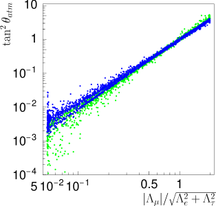
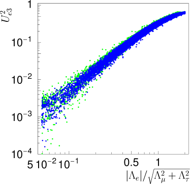
are required for BRpV to fit the data. We cannot set all the $\Lambda_{i}$ equal, because in this case $U_{e3}$ would be too large contradicting the CHOOZ, as shown in Fig. 2 a).

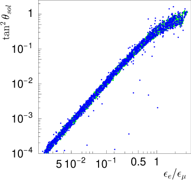
Figure 2: a) Atmospheric angle as a function of $|\Lambda_{\mu}|/\sqrt{\Lambda^{2}_{e}+\Lambda^{2}_{\tau}}$. b) $U^{2}_{e3}$ as a function of $|\Lambda_{e}|/\sqrt{\Lambda^{2}_{\mu}+\Lambda^{2}_{\tau}}$.

We have shown that even a very small deviation from universality (less then 1%) of the soft parameters at the GUT scale allows for

$$\frac{\epsilon_{e}}{\epsilon_{\mu}}\not=\frac{\Lambda_{e}}{\Lambda_{\mu}}$$ (21)

Then we can have at the same time small $U_{e3}^{2}$ determined by $\Lambda_{e}/\Lambda_{\mu}$ as in Fig. 2 a) and large $\tan^{2}(\theta_{\mathsc{sol}})$ determined by $\epsilon_{e}/\epsilon_{\mu}$ as in Fig. 2 b). After the Kamland and SNO salt results, this is the only scenario consistent with the data.

2.4 Approximate formulas for the solar mass and mixing

In all the previous analysis we used a numerical program to evaluate the one-loop masses and mixings. It is however desirable to have analytical approximate results that can give us quickly the most important contributions. We have identified that these are the bottom-sbottom loops and the charged scalar-charged fermion loops. Then, by expanding in powers of the small R-Parity breaking parameters $\epsilon_{i}$, we get approximate formulas for the solar mass scale and mixing angle as we will explain below.

2.4.1 Bottom-sbottom loops

As an example, we give the result from the bottom-sbottom loop diaz:2003as ,

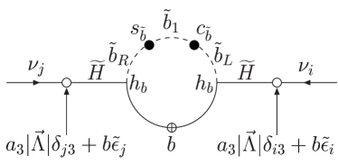
$$\Delta M_{ij} = -{\frac{N_{c}m_{b}}{16\pi^{2}}}2s_{\tilde{b}}c_{\tilde{b}}h_{b}^{2}\Delta B_{0}^{\tilde{b}_{1}\tilde{b}_{2}}\left[\frac{\tilde{\epsilon}_{i}\tilde{\epsilon}_{j}}{\mu^{2}}+a_{3}b\left(\tilde{\epsilon}_{i}\delta_{j3}+\tilde{\epsilon}_{j}\delta_{i3}\right)|\vec{\Lambda}|\right.$$ (22)

$$\hskip 113.81102pt\left.+\left(a_{3}^{2}+\frac{a_{L}a_{R}}{h^{2}_{b}}\right)\delta_{i3}\delta_{j3}|\vec{\Lambda}|^{2}\right]\,,$$

where $\widetilde{\epsilon}_{i}$ are the $\epsilon_{i}$ in the basis where the tree level neutrino mass matrix is diagonal,

$$\widetilde{\epsilon}_{i}=\left(V_{\nu}^{(0)T}\right)^{ij}\epsilon_{j}\,,$$ (23)

the $a_{i}$ are functions of the SUSY parameters, and

$$\Delta B_{0}^{\tilde{b}_{1}\tilde{b}_{2}}=B_{0}(0,m_{b}^{2},m_{\tilde{b}_{1}}^{2})-B_{0}(0,m_{b}^{2},m_{\tilde{b}_{2}}^{2})\,.$$ (24)

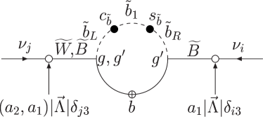
where the $B_{0}$ are the Passarino–Veltman loop functions passarino:1979jh . The different contributions can be understood as coming from different types of insertions as shown in Fig. 3. In this figure open circles correspond to small R-parity violating projections, full circles to R-parity conserving projections, and open circles with a cross inside to mass insertions which flip chirality. With this understanding one can make a one to one correspondence between Eq. (22) and Fig. 3.

Figure 3: Bottom-sbottom loop and different types of insertions.

2.4.2 Simplified approximation formulas

In the basis where the tree-level neutrino mass matrix is diagonal the mass matrix at one–loop level can be written as

$$\widetilde{m}_{\nu}=V_{\nu}^{(0)T}m_{\nu}V_{\nu}^{(0)}=\left(\begin{array}[]{ccc}c_{1}\widetilde{\epsilon}_{1}\widetilde{\epsilon}_{1}&c_{1}\widetilde{\epsilon}_{1}\widetilde{\epsilon}_{2}&c_{1}\widetilde{\epsilon}_{1}\widetilde{\epsilon}_{3}\\[5.69054pt] c_{1}\widetilde{\epsilon}_{2}\widetilde{\epsilon}_{1}&c_{1}\widetilde{\epsilon}_{2}\widetilde{\epsilon}_{2}&c_{1}\widetilde{\epsilon}_{2}\widetilde{\epsilon}_{3}\\ c_{1}\widetilde{\epsilon}_{3}\widetilde{\epsilon}_{1}&c_{1}\widetilde{\epsilon}_{3}\widetilde{\epsilon}_{2}&c_{0}|\vec{\Lambda}|^{2}+c_{1}\widetilde{\epsilon}_{3}\widetilde{\epsilon}_{3}\end{array}\right)+\cdots$$

where

$$c_{0} = \frac{M_{1}g^{2}+M_{2}{g^{\prime}}^{2}}{4\,\textrm{det}({\cal M}_{\chi^{0}})}$$ (25)

$$c_{1} = \frac{3}{16\pi^{2}}\,\sin(2\theta_{\tilde{b}})\,m_{b}\,\Delta B_{0}^{\tilde{b}_{2}\tilde{b}_{1}}\ \frac{1}{\mu^{2}}$$ (26)

The dots in Eq. (2.4.2) correspond to the terms that are not proportional to the $\tilde{\epsilon}_{i}\times\tilde{\epsilon}_{j}$ structure, as can be seen from Eq. (22). Assuming that the bottom-sbottom loop dominates, the $\tilde{\epsilon}_{i}\times\tilde{\epsilon}_{j}$ structure is dominant, and the matrix can be diagonalized approximately under the condition

$$x\equiv\frac{c_{1}|\vec{\widetilde{\epsilon}}|^{2}}{c_{0}|\vec{\Lambda}|^{2}}\ll 1$$ (27)

Then we get

$$m_{\nu_{2}}\simeq\frac{3}{16\pi^{2}}\sin(2\theta_{\tilde{b}})m_{b}\Delta B_{0}^{\tilde{b}_{2}\tilde{b}_{1}}\ \frac{({\tilde{\epsilon}}_{1}^{2}+{\tilde{\epsilon}}_{2}^{2})}{\mu^{2}}$$ (28)

and

$$\tan^{2}\theta{sol}=\frac{\widetilde{\epsilon}_{1}^{2}}{\widetilde{\epsilon}_{2}^{2}}$$ (29)

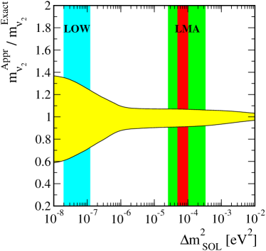
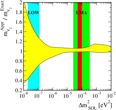
The results for the masses are presented in Fig. 4.

Figure 4: Comparison between the simplified analytical formulas and numerical results for the solar mass. In the left panel the LSP=$\chi^{0}$ while in the right panel the LSP=$\tilde{\tau}$. The red (dark) band corresponds to the latest neutrino data maltoni:2004ei .

On the left panel we have the data set where the neutralino is the LSP while on the right panel the LSP is the stau. We see that the agreement is fairly good, particularly in the region allowed by the present data.

2.5 Probing Neutrino Mixing via SUSY Decays

After having shown, in the previous sections, that the BRpV model produces an hierarchical mass spectrum for the neutrinos that can accommodate the present data for neutrino masses and mixings, we now turn to accelerator physics and will show how the neutrino properties can be probed by looking at the decays of supersymmetric particles.

If R-parity is broken the LSP will decay. If the LSP decays then cosmological and astrophysical constraints on its nature no longer apply. Thus, within R-parity violating SUSY, a priori any superparticle could be the LSP. In the constrained version of the MSSM (mSUGRA boundary conditions) one finds only two candidates for the LSP, namely the lightest neutralino or one of the right sleptons, in particular the right scalar tau. Therefore we will consider below these two cases. However, if we depart from the mSUGRA scenario, it has been shown recentlyhirsch:2003fe that the LSP can be of any other type, like a squark, gluino, chargino or even a scalar neutrino.

2.5.1 Probing Neutrino Mixing via Neutralino Decays

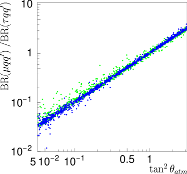
If the neutralino is the LSP and R-parity is broken, it will be unstable and it will decay. It was shown in Ref. porod:2000hv , that the neutralino decays well inside the detectors and that the visible decay channels are quite large. We have shown in the previous sections that the ratios $|\Lambda_{i}/\Lambda_{j}|$ and $|\epsilon_{i}/\epsilon_{j}|$ were very important in the choice of solutions for the neutrino mixing angles. What is exciting now, is that these ratios can be measured in accelerator experiments. In the left panel of Fig. 5 we show the ratio of branching ratios for semileptonic neutralino decays into muons and taus: $BR(\chi\to\mu q^{\prime}\bar{q})/BR(\chi\to\tau q^{\prime}\bar{q}$) as function of $\tan^{2}\theta_{\mathsc{atm}}$. We can see that there is a strong correlation. The spread in this figure can in fact be explained by the fact that we do not know the SUSY parameters and are scanning over the allowed parameter space. This is illustrated in the right panel where we considered that SUSY was already discovered with the following values for the parameters,

$$M_{2}=120\,{\rm GeV},\mu=m_{0}=500\,{\rm GeV},\tan\beta=5,A=-500\,{\rm GeV}.$$ (30)

Figure 5: Ratios of semileptonic branching ratios as a function of $\tan^{2}\theta_{\mathsc{atm}}$. On the left for random SUSY values and on the right for the SUSY point of Eq. (30).

2.5.2 Probing Neutrino Mixing via Charged Lepton Decays

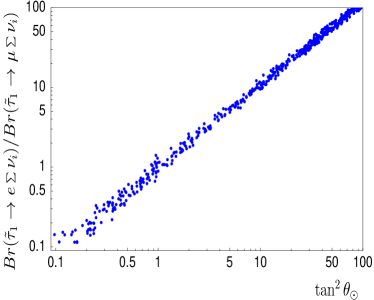
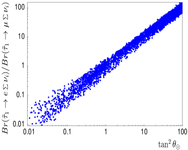
After considering the case of the LSP being the neutralino, for completeness, we have also studied hirsch:2002ys the case where a charged scalar lepton, most probably the scalar tau, is the LSP. We have considered the production and decays of ${\tilde{\tau}}$, ${\tilde{e}}$ and ${\tilde{\mu}}$, and have shown that also for the case of charged sleptons as LSPs they will decay well inside the detector. We can correlate branching ratios with neutrino properties. This is shown in Fig. 6 where the branching ratios of the scalar tau show a strong correlation with the solar angle.

Figure 6: Ratios of branching ratios for scalar tau decays versus $\tan^{2}\theta_{\odot}$. The left panel shown all data points, the right one refers only to data points with $\epsilon_{2}/\epsilon_{3}$ restricted to the range [0.9,1.1].

2.5.3 Other LSP decays

As we discussed in the introduction to this section, if we depart from the mSUGRA scenario, then the LSP can be of other type, like a squark, gluino, chargino or even a scalar neutrino, as it has been shown recently in Ref. hirsch:2003fe . As the decays of these LSP’s will always depend on the parameters that violate R-parity and induce neutrino masses and mixings, it is possible to correlate branching ratios to the neutrino properties. This is shown in Fig. 7 taken from Ref hirsch:2003fe .

Figure 7: Left panel: ratios of branching ratios for chargino decays versus $(\Lambda_{2}/\Lambda_{3})^{2}$; Right panel: ratios of branching ratios for squark decays versus $\tan^{2}\theta\mathsc{sol}$. These plots were taken from Ref. hirsch:2003fe .

On the left panel we consider the case of chargino decays and show $BR(\tilde{\chi}^{+}\rightarrow\mu\bar{c}c)/BR(\tilde{\chi}^{+}\rightarrow\tau\bar{c}c)$ as a function of the ratio $(\Lambda_{2}/\Lambda_{3})^{2}$. As we saw, this last ratio is correlated with the atmospheric angle. So, by looking at the chargino decays one can test the atmospheric mixing angle. On the right panel we show a very strong correlation for the solar mixing angle obtained hirsch:2003fe with the decays of squarks. Many other correlations can be obtained making the model over constrained. So, in summary, no matter what supersymmetric particle is the LSP, measurements of branching ratios at future accelerators will provide a definite test of the BRpV model as a viable model for explaining the neutrino properties.

3 Spontaneous Broken R-Parity Model

3.1 The Model

The most general superpotential for the SBRp model is masiero:1990uj , romao:1992vu , romao:1992ex , hirsch:2004rw

$${\cal W} \hskip-11.38109pt=\hskip-11.38109pt \varepsilon_{ab}\Big{(}h_{U}^{ij}\widehat{Q}_{i}^{a}\widehat{U}_{j}\widehat{H}_{u}^{b}+h_{D}^{ij}\widehat{Q}_{i}^{b}\widehat{D}_{j}\widehat{H}_{d}^{a}+h_{E}^{ij}\widehat{L}_{i}^{b}\widehat{E}_{j}\widehat{H}_{d}^{a}$$ (31)

$$+h_{\nu}^{ij}\widehat{L}_{i}^{a}\widehat{\nu}^{c}_{j}\widehat{H}_{u}^{b}\!-{\hat{\mu}}\widehat{H}_{d}^{a}\widehat{H}_{u}^{b}\!-(h_{0}\widehat{H}_{d}^{a}\widehat{H}_{u}^{b}+\delta^{2})\widehat{\Phi}\Big{)}$$

$$+\hskip 14.22636pth^{ij}\widehat{\Phi}\widehat{\nu}^{c}_{i}\widehat{S}_{j}+M_{R}^{ij}\widehat{\nu}^{c}_{i}\widehat{S}_{j}+\frac{1}{2}M_{\Phi}\widehat{\Phi}^{2}+\frac{\lambda}{3!}\widehat{\Phi}^{3}$$

The first three terms together with the ${\hat{\mu}}$ term define the R-parity conserving MSSM, the terms in the last row only involve the SU(2) $\otimes$ U(1) singlet superfields $({\nu^{c}}_{i},S_{i},\Phi)$ carrying a conserved lepton number assigned as $(-1,1,0)$, while the remaining terms couple the singlets to the MSSM fields. To this we will have to add the soft SUSY breaking terms in the usual way hirsch:2004rw .

3.2 Pattern of spontaneous symmetry breaking

The spontaneous breaking of $R_{P}$ is driven by nonzero vevs for the scalar neutrinos. The scale characterizing $R_{P}$ breaking is set by the isosinglet vevs,

$$\left\langle\tilde{\nu^{c}}\right\rangle=\frac{v_{R}}{\sqrt{2}},\quad\left\langle\tilde{S}\right\rangle=\frac{v_{S}}{\sqrt{2}},\quad\left\langle\Phi\right\rangle=\frac{v_{\Phi}}{\sqrt{2}}$$ (32)

We also have very small left-handed sneutrino vacuum expectation values

$$\left\langle\tilde{\nu}_{Li}\right\rangle=\frac{v_{Li}}{\sqrt{2}}$$ (33)

The electroweak breaking is driven by

$$\left\langle{H_{u}}\right\rangle=\frac{v_{u}}{\sqrt{2}},\quad\left\langle{H_{d}}\right\rangle=\frac{v_{d}}{\sqrt{2}}$$ (34)

with $v^{2}=v_{u}^{2}+v_{d}^{2}+\sum_{i}v_{Li}^{2}$ and $m_{W}^{2}=\frac{g^{2}v^{2}}{4}$. The spontaneous breaking of R–parity also entails the spontaneous violation of total lepton number. This implies that the majoron

$$J=\mathrm{Im}\left[\displaystyle\frac{v_{L}^{2}}{Vv^{2}}(v_{u}H_{u}-v_{d}H_{d})+\sum_{i}\frac{v_{Li}}{V}\tilde{\nu_{i}}+\frac{v_{S}}{V}S-\frac{v_{R}}{V}\tilde{\nu^{c}}\right]$$ (35)

remains massless, as it is the Nambu-Goldstone boson associated to the breaking of lepton number.

3.3 Neutrino-Neutralino-Singlino mass matrix

For simplicity we choose only one generation of singlet superfields. Then in the basis $(-i\lambda^{\prime},-i\lambda^{3},{\tilde{H}_{d}},{\tilde{H}_{u}},\nu_{e},\nu_{\mu},\nu_{\tau},\nu^{c},S,\tilde{\Phi})$ the neutrino/neutralino mass matrix is $10\times 10$,

$$\mathbf{M_{N}}=\left(\begin{array}[]{lllll}\mathbf{M_{\chi^{0}}}&\mathbf{m_{\chi^{0}\nu}}&\mathbf{m_{\chi^{0}\nu^{c}}}&\mathbf{0}&\mathbf{m_{\chi^{0}\Phi}}\\ \\ \mathbf{m^{T}_{\chi^{0}\nu}}&\mathbf{0}&\mathbf{m_{D}}&\mathbf{0}&\mathbf{0}\\ \\ \mathbf{m^{T}_{\chi^{0}\nu^{c}}}&\mathbf{m^{T}_{D}}&\mathbf{0}&\mathbf{M_{\nu^{c}S}}&\mathbf{M_{\nu^{c}\Phi}}\\ \\ \mathbf{0}&\mathbf{0}&\mathbf{M^{T}_{\nu^{c}S}}&\mathbf{0}&\mathbf{M_{S\Phi}}\\ \\ \mathbf{m^{T}_{\chi^{0}\Phi}}&\mathbf{0}&\mathbf{M^{T}_{\nu^{c}\Phi}}&\mathbf{M^{T}_{S\Phi}}&\mathbf{M_{\Phi}}\end{array}\right)$$ (36)

where $\mathbf{M_{\chi^{0}}}$ is the usual MSSM neutralino mass matrix, and

$$\mathbf{m^{T}_{\chi^{0}\nu}}\hskip-2.84526pt=\hskip-2.84526pt\left(\!\begin{array}[]{llll}-\frac{1}{2}g^{\prime}v_{Le}&\frac{1}{2}gv_{Le}&0&\epsilon_{e}\\[5.69054pt] -\frac{1}{2}g^{\prime}v_{L\mu}&\frac{1}{2}gv_{L\mu}&0&\epsilon_{\mu}\\[5.69054pt] -\frac{1}{2}g^{\prime}v_{L\tau}&\frac{1}{2}gv_{L\tau}&0&\epsilon_{\tau}\end{array}\!\right)$$ (37)

$$(\mathbf{m_{D}})_{i}=\frac{1}{\sqrt{2}}h_{\nu}^{i}v_{u}$$ (38)

with an effective “bilinear R–parity” parameter

$$\epsilon_{i}=\frac{1}{\sqrt{2}}h_{\nu}^{i}v_{R}$$ (39)

The other block matrices in Eq. (36) can found explicitly in Ref.hirsch:2004rw .

3.4 The effective neutrino mass matrix

The exact diagonalization of Eq. (36) can only be done numerically. However due to the smallness of the neutrino masses, an effective neutrino mass matrix can be cast into a very simple form

$$(\mathbf{m_{\nu\nu}^{\rm eff}})_{ij}=a\Lambda_{i}\Lambda_{j}+b(\epsilon_{i}\Lambda_{j}+\epsilon_{j}\Lambda_{i})+c\epsilon_{i}\epsilon_{j}.$$ (40)

where the model dependence in hidden in the parameters $a,b,c$. The effective bilinear R–parity violating parameters $\epsilon_{i}$ and $\Lambda_{i}$, are given in Eq. (39) and Eq. (11), respectively. This equation resembles very closely the result for the BRpV model once the dominant 1-loop corrections are taken into account. The tree-level result of the explicit bilinear model can be recovered in the limit $M_{R},M_{\Phi}\to\infty$.

$$a=\displaystyle\frac{g^{2}M_{1}+g^{\prime 2}M_{2}}{4{\rm Det}\mathbf{M_{\chi^{0}}}},\quad b=0,\quad c=0$$ (41)

In this limit only one non-zero neutrino mass remains. The relative size of the coefficient $c$ compared to the corresponding 1-loop coefficient dictates if the 1-loop corrections or the contribution from the singlet fields are more important. Both extremes can be realized in our model. Large branching ratios of the Higgs into invisible final states require sizable values of $h$ and $h_{0}$. Then the “singlino” contribution dominates.

3.5 The Neutral Scalar Bosons Mass Matrix

The $8\times 8$ scalar mass matrix is a symmetric matrix that in the basis $(H_{d}^{0},H_{u}^{0},\tilde{\nu}_{i},\Phi,\tilde{S},\tilde{\nu}^{c})$ takes the form,

$$M^{S^{2}}=\left[\begin{array}[]{lll}M^{S^{2}}_{HH}&M^{S^{2}}_{H\widetilde{L}}&M^{S^{2}}_{HS}\\[12.80373pt] M^{S^{2}}_{H\widetilde{L}}\!{}^{T}&M^{S^{2}}_{\widetilde{L}\widetilde{L}}&M^{S^{2}}_{\widetilde{L}S}\\[12.80373pt] M^{S^{2}}_{HS}\!{}^{T}&M^{S^{2}}_{\widetilde{L}S}\!{}^{T}&M^{S^{2}}_{SS}\end{array}\right]$$ (42)

written in terms of block matrices that can be found in Ref.hirsch:2004rw . The pseudo–scalar mass matrix has a similar form. In practice they are quite complicated and have to be diagonalized numerically. The most important feature of the pseudo–scalar mass matrix is the existence of two massless Goldstone bosons, corresponding to the spontaneous breaking of gauge symmetry (the usual Goldstone $G_{0}$ “eaten” by the $Z^{0}$) and to the spontaneous breaking of R–parity, the majoron $J$. In the basis

$$A^{\prime}_{0}=(H_{d}^{0I},H_{u}^{0I},\tilde{\nu}^{1I},\tilde{\nu}^{2I},\tilde{\nu}^{3I},\Phi^{I},\tilde{S}^{I},\tilde{\nu}^{cI})$$ (43)

we have

$$G_{0} = (N_{0}\,v_{d},-N_{0}\,v_{u},N_{0}\,v_{L1},N_{0}\,v_{L2},N_{0}\,v_{L3},0,0,0)$$

$$J = (-N_{1}v_{d},N_{1}v_{u},N_{2}v_{L1},N_{2}v_{L2},N_{2}v_{L3},0,N_{3}v_{S},-N_{3}v_{R})$$ (44)

where the $N_{i}$ are normalization constants. It can easily be checked that they are orthogonal $G_{0}\cdot J=0$.

3.6 Higgs Boson Production

Supersymmetric Higgs bosons can be produced at an $e^{+}e^{-}$ collider via the so–called Bjorken process,

$${\cal L}_{HZZ}=\displaystyle\sum_{i=1}^{8}(\sqrt{2}G_{F})^{1/2}M_{Z}^{2}Z_{\mu}Z^{\mu}\eta_{i}H_{i}$$ (45)

where the $\eta_{i}$ are combinations of the doublet scalars vevs and rotation matrices:

$$\eta_{i}=\frac{v_{d}}{v}R^{S}_{i1}+\frac{v_{u}}{v}R^{S}_{i2}+\sum_{j=1}^{3}\frac{v_{Lj}}{v}R^{S}_{ij+2}$$ (46)

In comparison with the SM the coupling of the lightest CP–even Higgs boson to the $Z$ is reduced by a factor

$$\eta\equiv\eta_{1}\leq 1.$$ (47)

In the MSSM we have $\eta=\sin(\beta-\alpha)$.

3.7 Higgs Boson Decay

We are interested here in the ratio

$$R_{Jb}=\displaystyle\frac{\Gamma(h\to JJ)}{\Gamma(h\to b\bar{b})}$$ (48)

of the invisible decay to the SM decay into b-jets. These decay widths are easily obtained hirsch:2004rw ,

$$\Gamma(h\to JJ)=\displaystyle\frac{g_{hJJ}^{2}}{32\pi m_{h}}$$ (49)

and

$$\Gamma(h\to b\bar{b})=\displaystyle\frac{3G_{F}\sqrt{2}}{8\pi}\,\left(R^{S}_{11}\right)^{2}\,m_{h}\,m_{b}^{2}\left[1-4\left(\frac{m_{b}}{m_{h}}\right)^{2}\right]^{3/2}$$ (50)

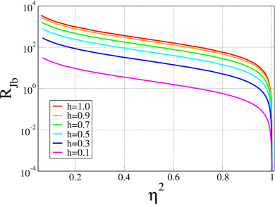
We want to look at situations where $R_{Jb}>1$, but that at the same time the Higgs boson is produced at a reasonable rate, which means that $\eta$ parameter should not be too small.

3.8 Scanning Strategy

As the model has a large number of parameters we have to follow a scanning strategy that can put in evidence the possibility of the Higgs boson decaying invisibly. This is achieved by fixing as many parameters as we can. Without loss of generality we then fix the MSSM parameters to the SPS1a benchmark point:

$$m_{0}=100\rm{GeV},\quad m_{1/2}=250\rm{GeV},\quad\tan\beta=10$$

$$A_{0}=-100\rm{GeV},\quad\mu<0$$ (51)

For the singlet parameters we choose to start with

$$v_{R}=v_{S}=v_{\Phi}=-150\mathrm{GeV}$$ (52)

$$M_{R}=-M_{\Phi}=\delta=10^{3}\mathrm{GeV}$$

$$h=0.8\ ,h_{0}=-0.15\ ,\lambda=0.1$$

and then perform variations around these values in a controlled way. Finally the explicit bilinear parameters, $\epsilon_{i}$ and $\Lambda_{i}$, are fixed approximately such that neutrino masses and mixing angles are in agreement with experimental data.

3.9 Numerical results: General Superpotential

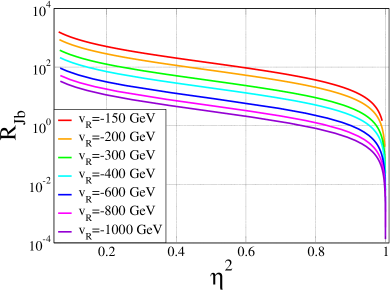
In Fig. 8 we show the plot of $R_{Jb}$ as a function of $\eta^{2}$. On the left panel we kept $h$ constant and varied continuously the other singlet parameters, while on the right panel the vevs were kept. We see that it is indeed possible to achieve, at the same time, both large branching ratio into the invisible mode ($h\to JJ$), and large production cross sections.

Figure 8: $R_{Jb}$ as a function of $\eta^{2}$: a) For constant values of $h$. b) For constant values of $v_{R}=v_{S}$.

In Ref.hirsch:2004rw a complete analysis of the parameter space where this happens is presented.

4 Conclusions

The BRpV model is a simple extension of the MSSM that leads to a very rich phenomenology. We have calculated the one–loop corrected masses and mixings for the neutrinos in a completely consistent way, including the RG equations and correctly minimizing the potential. We have shown that it is possible to get easily maximal mixing for the atmospheric neutrinos and large angle MSW, as it is preferred by the present neutrino data. We have also obtained approximate formulas for the solar mass and solar mixing angle, that we found to be very good, precisely in the region of parameters favored by this data.

We emphasize that the LSP decays inside the detectors, thus leading to a very different phenomenology than the MSSM. No matter what supersymmetric particle is the LSP measurements of branching ratios at future accelerators will provide a definite test of the BRpV model as a viable model for explaining the neutrino properties.

We have also discussed the possibility of invisibly decaying Higgs boson in the context of the SBRp model. One of the neutral CP-odd scalars in this model, is the Nambu-Goldstone boson associated to the breaking of lepton number, the majoron $J$. Neutrino masses and mixings can easily be explained. In contrast to the MSSM, where the Higgs boson can decay invisibly only to supersymmetric states, in our case the Higgs boson can decay mainly invisibly through the decay $h\to JJ$. As a result, our analysis indicates that invisibly decaying Higgs bosons should be an important topic in the agenda of future accelerators, such as the Large Hadron Collider and the Next Linear Collider.

References

• [1] Super-Kamiokande, Y. Fukuda et al., Phys. Rev. Lett. 81, 1562 (1998), [hep-ex/9807003].
• [2] SNO, Q. R. Ahmad et al., Phys. Rev. Lett. 89, 011301 (2002), [nucl-ex/0204008].
• [3] KamLAND, K. Eguchi et al., Phys. Rev. Lett. 90, 021802 (2003), [hep-ex/0212021].
• [4] M. Maltoni, T. Schwetz, M. A. Tortola and J. W. F. Valle, New J. Phys. 6, 122 (2004), [hep-ph/0405172].
• [5] M. Gell-Mann, P. Ramond and R. Slansky, (1979), Print-80-0576 (CERN).
• [6] T. Yanagida, (1979), ed. Sawada and Sugamoto (KEK, 1979).
• [7] R. N. Mohapatra and G. Senjanovic, Phys. Rev. D23, 165 (1981).
• [8] Y. Chikashige, R. N. Mohapatra and R. D. Peccei, Phys. Lett. B98, 265 (1981).
• [9] J. Schechter and J. W. F. Valle, Phys. Rev. D22, 2227 (1980).
• [10] R. N. Mohapatra and J. W. F. Valle, Phys. Rev. D34, 1642 (1986).
• [11] A. Zee, Phys. Lett. B93, 389 (1980).
• [12] K. S. Babu, Phys. Lett. B203, 132 (1988).
• [13] C. S. Aulakh and R. N. Mohapatra, Phys. Lett. B119, 136 (1982).
• [14] M. A. Diaz, J. C. Romao and J. W. F. Valle, Nucl. Phys. B524, 23 (1998), [hep-ph/9706315].
• [15] M. A. Diaz, M. Hirsch, W. Porod, J. C. Romao and J. W. F. Valle, Phys. Rev. D68, 013009 (2003), [hep-ph/0302021].
• [16] M. Hirsch, M. A. Diaz, W. Porod, J. C. Romao and J. W. F. Valle, Phys. Rev. D62, 113008 (2000), [hep-ph/0004115], Err-ibid.D65:119901,2002.
• [17] J. C. Romao, M. A. Diaz, M. Hirsch, W. Porod and J. W. F. Valle, Phys. Rev. D61, 071703 (2000), [hep-ph/9907499].
• [18] M. Hirsch and J. W. F. Valle, New J. Phys. 6, 76 (2004), [hep-ph/0405015].
• [19] M. Hirsch, W. Porod, J. C. Romao and J. W. F. Valle, Phys. Rev. D66, 095006 (2002), [hep-ph/0207334].
• [20] W. Porod, M. Hirsch, J. Romao and J. W. F. Valle, Phys. Rev. D63, 115004 (2001), [hep-ph/0011248].
• [21] D. Restrepo, W. Porod and J. W. F. Valle, Phys. Rev. D64, 055011 (2001), [hep-ph/0104040].
• [22] M. Hirsch and W. Porod, Phys. Rev. D68, 115007 (2003), [hep-ph/0307364].
• [23] A. Masiero and J. W. F. Valle, Phys. Lett. B251, 273 (1990).
• [24] J. C. Romao, C. A. Santos and J. W. F. Valle, Phys. Lett. B288, 311 (1992).
• [25] M. Shiraishi, I. Umemura and K. Yamamoto, Phys. Lett. B313, 89 (1993).
• [26] J. C. Romao and J. W. F. Valle, Nucl. Phys. B381, 87 (1992).
• [27] J. C. Romao, F. de Campos and J. W. F. Valle, Phys. Lett. B292, 329 (1992), [hep-ph/9207269].
• [28] F. De Campos, J. W. F. Valle, A. Lopez-Fernandez and J. C. Romao, hep-ph/9405382.
• [29] F. de Campos, O. J. P. Eboli, J. Rosiek and J. W. F. Valle, Phys. Rev. D55, 1316 (1997), [hep-ph/9601269].
• [30] M. Hirsch, J. C. Romao, J. W. F. Valle and A. Villanova del Moral, Phys. Rev. D70, 073012 (2004), [hep-ph/0407269].
• [31] F. de Campos, M. A. Garcia-Jareno, A. S. Joshipura, J. Rosiek and J. W. F. Valle, Nucl. Phys. B451, 3 (1995), [hep-ph/9502237].
• [32] A. G. Akeroyd, M. A. Diaz, J. Ferrandis, M. A. Garcia-Jareno and J. W. F. Valle, Nucl. Phys. B529, 3 (1998), [hep-ph/9707395].
• [33] T. Banks, Y. Grossman, E. Nardi and Y. Nir, Phys. Rev. D52, 5319 (1995), [hep-ph/9505248].
• [34] G. Passarino and M. J. G. Veltman, Nucl. Phys. B160, 151 (1979).
• [35] B. Mukhopadhyaya, S. Roy and F. Vissani, Phys. Lett. B443, 191 (1998), [hep-ph/9808265].