Kinetic and Chemical Equilibration
in Scalar $\varphi^{4}$ Theory

Abstract

Approximations based on the 2PI effective action are used to investigate the process of equilibration in $\varphi^{4}$ theory in 3+1 dimensions, both in the symmetric and broken phase. A special emphasis is put on the study of the kinetic and chemical equilibration.

1 Introduction

To establish the formation of a thermalized quark-gluon plasma during a heavy-ion collision it is crucial to determine the time scales involved in the equilibration of the initial fireball. The hydrodynamic description of the experiments suggests early thermalization [1], which seems to contradict traditional perturbative estimates [2]. The resolution of this puzzle has spurred the development of techniques to understand the microscopic dynamical processes leading to equilibration.

A powerful formalism to study out-of-equilibrium dynamics from first principles is the 2PI effective action. It provides an exact representation of a given theory in terms of a functional depending solely on the connected one- and two-point functions. Approximate equations describing the time evolution of these correlators can be derived from a variational principle on the functional. The main interest of the 2PI effective action as a framework to obtain evolution equations is the fact that the global symmetries of the theory are respected [3]. In particular, the evolution equations guarantee energy conservation, which is an important feature when studying out-of-equilibrium processes. They also seem to be free of the secular instabilities that plague traditional perturbative approaches.

In recent years, approximations based on the 2PI effective action have been applied succesfully to the study of far-from-equilibrium dynamics and equilibration. Most studies have been carried out in scalar theories, both in 1+1 [4, 5, 6] and 2+1 dimensions [7], and in Yukawa theory in 3+1 dimensions [8]. The application of 2PI effective action methods to gauge theories, however, is not straightforward due to a residual dependence on the choice of gauge condition [9] and the difficulty of implementing properly a numerical discretisation. In this work we extend to 3+1 dimensions previous studies of equilibration in scalar theory, investigating, in addition, the behavior in the broken phase. More information can be found in [10].

2 2PI Effective action and evolution equations

For the scalar theory given by the action in the form

$$S[\varphi]=\int d^{4}x\,\int d^{4}y\frac{1}{2}\varphi(x)G_{0}^{-1}(x,y)\varphi(y)-\frac{\lambda}{4!}\varphi(x)^{4}$$ (1)

with $G_{0}^{-1}(x,y)=(-\partial_{x}^{2}-m^{2})\delta(x,y)$, the corresponding 2PI effective action is given by [11]

$$\Gamma_{\mbox{\scriptsize 2PI}}[\phi,G]=S[\phi]-\frac{i}{2}\mbox{Tr}\ln G+\frac{i}{2}\mbox{Tr}\Big{[}(G_{0}^{-1}-G^{-1})\cdot G\Big{]}+\Phi[\phi,G]$$ (2)

Here $\phi$ and $G$ correspond, respectively, to the full connected one- and two-point correlation functions. The functional $\Phi$ consists of an inifinite series of closed skeleton diagrams

$$i\Phi[\phi,G]=\frac{1}{4}\;\parbox[c]{20.0pt}{\begin{picture}(20.0,30.0)(0.0,0.0) \put(0.0,0.0){} \put(0.0,0.0){} \put(0.0,0.0){} \put(0.0,0.0){} \put(0.0,0.0){} \put(0.0,0.0){} \end{picture}}\;+\frac{1}{8}\;\parbox[c]{20.0pt}{\begin{picture}(20.0,30.0)(0.0,0.0) \put(0.0,0.0){} \put(0.0,0.0){} \put(0.0,0.0){} \end{picture}}\;+\frac{1}{12}\;\parbox[c]{45.0pt}{\begin{picture}(45.0,30.0)(0.0,0.0) \put(0.0,0.0){} \put(0.0,0.0){} \put(0.0,0.0){} \put(0.0,0.0){} \put(0.0,0.0){} \put(0.0,0.0){} \put(0.0,0.0){} \put(0.0,0.0){} \end{picture}}\;+\frac{1}{48}\;\parbox[c]{30.0pt}{\begin{picture}(30.0,30.0)(0.0,0.0) \put(0.0,0.0){} \put(0.0,0.0){} \put(0.0,0.0){} \put(0.0,0.0){} \end{picture}}\;+\ldots$$ (3)

where the lines correspond to $G$, the crosses to $\phi$ and the vertices to $-i\lambda$.

Evolution equations for the one- and two-point functions are obtained by a variational principle on the effective action $\Gamma_{\mbox{\scriptsize 2PI}}$, conveniently formulated using a real-time contour for the time integrations. One obtains

$$\frac{\delta\Gamma_{\mbox{\scriptsize 2PI}}[\phi,G]}{\delta G} =0\rightarrow\delta_{\mathcal{C}}(x,y)=\int_{\mathcal{C}}d^{4}z\,G_{0}^{-1}(x,z)G(z,y)+i\int_{\mathcal{C}}d^{4}z\,\Sigma(x,z)G(z,y)$$ (4)

$$\frac{\delta\Gamma_{\mbox{\scriptsize 2PI}}[\phi,G]}{\delta\phi} =0\rightarrow\left[\partial^{2}+m^{2}\right]\phi(x)=-\frac{\lambda}{6}\phi(x)^{3}+\frac{\delta\Phi[\phi,G]}{\delta\phi(x)},$$ (5)

with $\mathcal{C}$ being the integration time contour (see for instance [12]). The self-energy $\Sigma(x,y)$ is given by

$$\Sigma(x,y)=-2\frac{\delta\Phi[\phi,G]}{\delta G(y,x)}.$$ (6)

The exact evolution of $\phi$ and $G$ would be determined by solving these equations including the infinite series of diagrams in $\Phi[\phi,G]$. This is not possible to do, so one considers approximate evolution equations that result from taking only a finite set of diagrams, i.e. by truncating $\Phi[\phi,G]$ up to some order in a convenient expansion parameter. In our study we consider various truncations of the loop expansion of $\Gamma_{\mbox{\scriptsize 2PI}}$, summarized in Table 1.

Truncation	$i\Phi[\phi,G]$
Hartree approximation	$\parbox[c]{1.0pt}{\begin{picture}(1.0,25.0)(0.0,0.0) \end{picture}}\frac{1}{4}\parbox[c]{20.0pt}{\begin{picture}(20.0,20.0)(0.0,0.0) \put(0.0,0.0){} \put(0.0,0.0){} \put(0.0,0.0){} \put(0.0,0.0){} \put(0.0,0.0){} \put(0.0,0.0){} \end{picture}}+\frac{1}{8}\parbox[c]{20.0pt}{\begin{picture}(20.0,20.0)(0.0,0.0) \put(0.0,0.0){} \put(0.0,0.0){} \put(0.0,0.0){} \end{picture}}$
Two-loop approximation	$\parbox[c]{1.0pt}{\begin{picture}(1.0,25.0)(0.0,0.0) \end{picture}}\frac{1}{4}\parbox[c]{20.0pt}{\begin{picture}(20.0,20.0)(0.0,0.0) \put(0.0,0.0){} \put(0.0,0.0){} \put(0.0,0.0){} \put(0.0,0.0){} \put(0.0,0.0){} \put(0.0,0.0){} \end{picture}}+\frac{1}{8}\parbox[c]{20.0pt}{\begin{picture}(20.0,20.0)(0.0,0.0) \put(0.0,0.0){} \put(0.0,0.0){} \put(0.0,0.0){} \end{picture}}+\frac{1}{12}\;\parbox[c]{30.0pt}{\begin{picture}(30.0,20.0)(0.0,0.0) \put(0.0,0.0){} \put(0.0,0.0){} \put(0.0,0.0){} \put(0.0,0.0){} \put(0.0,0.0){} \put(0.0,0.0){} \put(0.0,0.0){} \put(0.0,0.0){} \end{picture}}$
“Basketball” approximation	$\parbox[c]{1.0pt}{\begin{picture}(1.0,25.0)(0.0,0.0) \end{picture}}\frac{1}{4}\parbox[c]{20.0pt}{\begin{picture}(20.0,20.0)(0.0,0.0) \put(0.0,0.0){} \put(0.0,0.0){} \put(0.0,0.0){} \put(0.0,0.0){} \put(0.0,0.0){} \put(0.0,0.0){} \end{picture}}+\frac{1}{8}\parbox[c]{20.0pt}{\begin{picture}(20.0,20.0)(0.0,0.0) \put(0.0,0.0){} \put(0.0,0.0){} \put(0.0,0.0){} \end{picture}}+\frac{1}{12}\;\parbox[c]{30.0pt}{\begin{picture}(30.0,20.0)(0.0,0.0) \put(0.0,0.0){} \put(0.0,0.0){} \put(0.0,0.0){} \put(0.0,0.0){} \put(0.0,0.0){} \put(0.0,0.0){} \put(0.0,0.0){} \put(0.0,0.0){} \end{picture}}+\frac{1}{48}\;\parbox[c]{30.0pt}{\begin{picture}(20.0,20.0)(0.0,0.0) \put(0.0,0.0){} \put(0.0,0.0){} \put(0.0,0.0){} \put(0.0,0.0){} \end{picture}}$

Table 1.: Truncations of the 2PI effective action.

In a real-scalar theory, the two-point functions defined on the time contour $\mathcal{C}$ can be written in terms of two independent components, which we take as

$$G_{\mathcal{C}}(x,y)=F(x,y)-\frac{i}{2}\mbox{sign}_{\mathcal{C}}(x_{0}-y_{0})\rho(x,y).$$ (7)

The functions $F$ and $\rho$ contain, respectively, statistical and spectral information about the system. They are real and satisfy the symmetry properties $F(x,y)=F(y,x)$ and $\rho(x,y)=-\rho(y,x)$, which make them very convenient for numerical implementation. In terms of these functions, the evolution equations look like

$$\left[\partial_{x}^{2}+M^{2}(x)\right]F(x,y) =\int_{0}^{x_{0}}dz_{0}\int d^{3}z\;\Sigma^{\rho}(x,z)F(z,y)-\int_{0}^{y_{0}}dz_{0}\int d^{3}z\;\Sigma^{F}(x,z)\rho(y,z),$$

$$\left[\partial_{x}^{2}+M^{2}(x)\right]\rho(x,y) =\int_{y_{0}}^{x_{0}}dz_{0}\int d^{3}z\;\Sigma^{\rho}(x,z)\rho(z,y),$$ (8)

$$\left[\partial_{x}^{2}+M^{2}(x)\right]\phi(x) =\frac{\lambda}{3}\phi(x)^{3}+\int_{0}^{x_{0}}dz_{0}\int d^{3}z\;\widetilde{\Sigma}^{\rho}(x,z)\phi(z),$$

where $M^{2}(x)=m^{2}+\frac{\lambda}{2}\phi(x)^{2}+\frac{\lambda}{2}F(x,x)$. For the Basketball approximation, we have

$$\Sigma^{F}(x,y) =\frac{\lambda^{2}}{2}\phi(x)\phi(y)\left[F^{2}(x,y)-\frac{\rho^{2}(x,y)}{4}\right]+\frac{\lambda^{2}}{6}F(x,y)\left[F^{2}(x,y)-\frac{3\rho^{2}(x,y)}{4}\right],$$

$$\Sigma^{\rho}(x,y) =\lambda^{2}\phi(x)\phi(y)\big{[}F(x,y)\rho(x,y)\big{]}+\frac{\lambda^{2}}{6}\rho(x,y)\left[3F^{2}(x,y)-\frac{\rho^{2}(x,y)}{4}\right],$$ (9)

$$\widetilde{\Sigma}^{\rho}(x,z) =-\frac{\lambda^{2}}{6}\rho(x,z)\left[3F(x,z)^{2}-\frac{\rho(x,z)^{2}}{4}\right].$$

We see from (8) that the evolution of $F$, $\rho$ and $\phi$ is determined by their values at previous times, which enter the equation in the form of memory integrals. For the two-loop approximation, the memory kernels are given by the first term in the RHS of (9), while for the Hartree approximation they vanish alltogether.

To solve set of coupled evolution equations (8) we need to specify a set of initial conditions. We consider a spatially homogeneous situation so that the correlators can be written in terms of their mode functions $F_{\mathbf{k}}(t,t^{\prime})$ and $\rho_{\mathbf{k}}(t,t^{\prime})$. The initial conditions are then given by the values and derivatives of the mode functions $F$, $\rho$ and $\phi$ at initial time. In the case of the spectral function $\rho$, these are specified by the property

$$\rho_{\mathbf{k}}(t,t)=0,\quad\partial_{,}\rho_{\mathbf{k}}(t,t^{\prime})\big{|}_{t=t^{\prime}}=1.$$ (10)

The initial conditions for $F$ are taken of the form

$$F_{\mathbf{k}}(t,t^{\prime})\big{|}_{t=t^{\prime}=0} =\frac{1}{\omega_{\mathbf{k}}}\left[n_{\mathbf{k}}+\frac{1}{2}\right],$$

$$\partial_{t}F_{\mathbf{k}}(t,t^{\prime})\big{|}_{t=t^{\prime}=0} =0,$$ (11)

$$\partial_{t}\partial_{t^{\prime}}F_{\mathbf{k}}(t,t^{\prime})\big{|}_{t=t^{\prime}=0} =\omega_{\mathbf{k}}\left[n_{\mathbf{k}}+\frac{1}{2}\right],$$

which are identical to the equilibrium free theory case, but with some arbitrary distribution function $n_{\mathbf{k}}$.

The evolution equations (8) are solved numerically by discretizing the theory on a space-time lattice with spacings $a_{t}\ll a$. The lattice provides a cut-off and regularizes the ultraviolet divergences present in the continuum limit, which are to be dealt with by renormalization. The continuum renormalization of approximations based on the 2PI effective action has been recently studied in detail (see for instance [13]). For our purpose it is sufficient to use an approximate renormalization that ensures that the relevant length scales in the simulations are larger than the lattice spacing $a$. For all the truncations of table (1) we take a perturbative version of the renormalization needed just for the Hartree case.

3 Symmetric Phase

We consider first the evolution of the system in the symmetric phase. We initialize the system far from equilibrium with a distribution of the form

$$n_{\mathbf{k}}=\eta\,\Theta({\mathbf{k}}^{2}_{\mbox{\scriptsize max}}-{\mathbf{k}}^{2})\Theta({\mathbf{k}}^{2}-{\mathbf{k}}^{2}_{\mbox{\scriptsize min}}),$$ (12)

which means that only modes with momenta in the range ${\mathbf{k}}_{\mbox{\scriptsize min}}^{2}<{\mathbf{k}}^{2}<{\mathbf{k}}^{2}_{\mbox{\scriptsize max}}$ are occupied. In the following we shall consider three diferent distributions: T1, T2 and T3, all with identical energy and T1 and T2 with similar initial particle number. The numerical evaluation of the evolution equations (8) is performed on a $16^{3}$ spatial lattice with spacing $am=0.7$ (in units of the renormalized mass $m$), time spacing $a_{t}m=0.07$ and coupling $\lambda=6$. To monitor the evolution of the system towards equilibrium we study the behavior of an effective quasiparticle distribution function and a dispersion relation, defined as

$$n_{\mathbf{k}}(t)+\frac{1}{2} =c_{\mathbf{k}}\sqrt{\partial_{t}\partial_{t^{\prime}}F_{\mathbf{k}}(t,t^{\prime})\big{|}_{t=t^{\prime}}\,F_{\mathbf{k}}(t,t)},$$ (13)

$$\omega_{\mathbf{p}}(t) =\sqrt{\partial_{t}\partial_{t^{\prime}}F_{\mathbf{k}}(t,t^{\prime})\big{|}_{t=t^{\prime}}\,/\,F_{\mathbf{k}}(t,t)}.$$ (14)

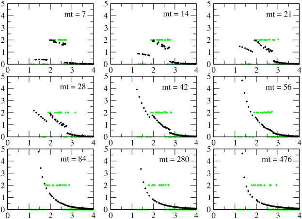
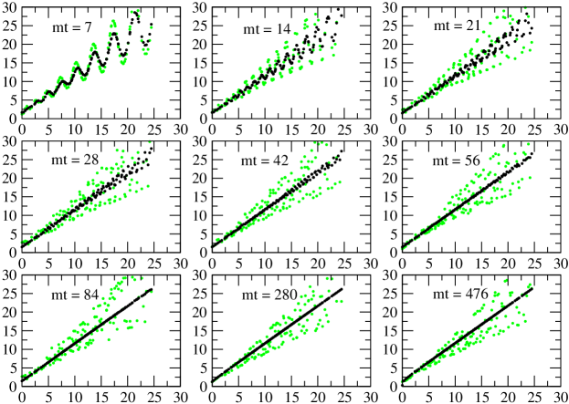
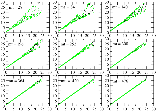
The evolution of the distribution $n_{\mathbf{k}}(t)$ and frequency $\omega_{\mathbf{p}}(t)$ is shown in Fig. 1 for the Hartree and Basketball approximations. In the Hartree case there is no inter-mode communication (no scattering), so the system does not equilibrate. In the Basketball case, the distribution and dispersion relation approach equilibrium profiles around $mt\approx 80$.

Fig. 1.: Evolution in time of the occupation numbers, $n_{\mathbf{k}}$ vs. $\omega_{\mathbf{k}}$ (left), and dispersion relation $\omega_{\mathbf{k}}^{2}$ vs. ${\mathbf{k}}^{2}$ (right), for an initial condition with $(\eta,\mathbf{k}^{2}_{\mbox{\tiny min}},\mathbf{k}^{2}_{\mbox{\tiny max}})=(2,2.04m^{2},6.12m^{2})$ (T1). We display the results of the “Basketball” (black dots) and the Hartree approximation (green/grey dots).

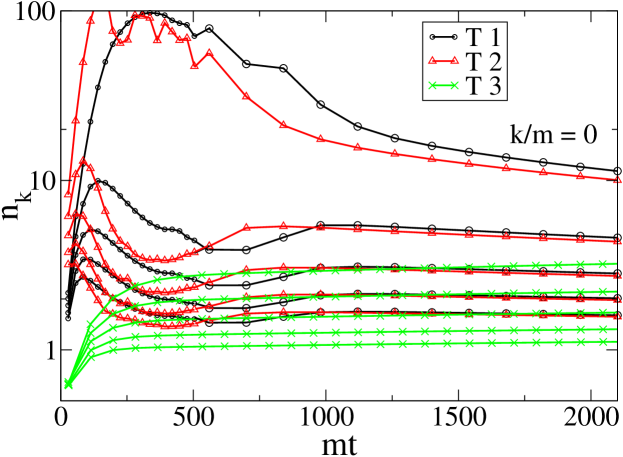
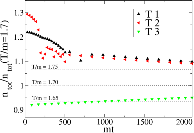
To find out if the system has indeed reached a universal equilibrium state, we study the evolution of individual modes for different initial conditions with identical energy density (see Fig. 3). One can see that the individual modes become roughly equilibrated at $mt\approx 1000$. Further on there is practically no inter-mode communication, so it is reasonable to say that kinetic equilibration has been established. There is still, however, a slow drift towards the complete equilibrium state, for which the mode distributions should agree for the various initial conditions. As one can see in Fig. 3, the evolution from the initial conditions $T1$ and $T3$ differs substantially even at $mt\sim 2000$, so the system is still far from complete equilibrium. The reason for the slow drift towards full equilibrium at later stages seems to be the fact that the system is not chemically equilibrated yet. This can be seen by plotting the evolution of the total particle number density $n_{\mbox{\tiny tot}}(t)=\int_{\mathbf{k}}n_{\mathbf{k}}(t)$, as shown in Fig. 3.

Fig. 2.: Evolution of individual modes for various initial conditions with same energy density (T1,T2 and T3).

Fig. 3.: Evolution of total particle number density $n_{\mbox{\tiny tot}}$ for (T1,T2 and T3)

One observes that the kinetically pre-equilibrated state remembers the initial particle number, and chemical equilibration occurs at a very slow rate.

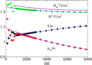
Fitting the distribution $n_{\mathbf{k}}(t)$ and frequency $\omega_{\mathbf{p}}(t)$ with an equilibrium form we can extract an effective temperature $T_{\mbox{\tiny eff}}(t)$, chemical potential $\mu_{\mbox{\tiny eff}}(t)$ and mass $M_{\mbox{\tiny eff}}(t)$ (see Fig. 4). Exponential fits for the effective temperature and chemical potential indicate that final equilibrium is reached at $mt\sim 10^{4-5}$. Comparing to the case in 2+1 dimensions [7], chemical equilibration seems to be much slower. The values of the effective masses seem to be roughly the same in the Basketball and Hartree approximations (also included in Fig. 4).

Fig. 4.: Evolution of effective mass, temperature and chemical potential (T1 case). Hartre mass $M_{H}$ is included for comparison.

4 Broken Phase

In the broken phase $\phi\neq 0$ and hence one can compare the approach to equilibrium between the two-loop and Basketball approximations. This is particularly interesting for the two-loop case, since perturbation theory predicts no on-shell scattering for the corresponding self-energy contribution. Thus a study of the time evolution using, for instance, Boltzmann-like equations will fail to show equilibration. An approach based on the 2PI effective action, however, includes higher-order self-energy contributions that do contain on-shell scattering. It also takes into account off-shell scattering, which can play an important role far away from equilibrium.

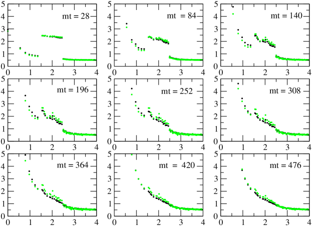
The system is initialized with a distribution function of the form (12). The mean field is taken at the tree level vacuum expectation value $\phi(t=0)=v_{\mbox{\tiny tree}}=\sqrt{6|m^{2}|/\lambda}$. For not so large couplings this is close to the actual variational value, so the time evolution of $\phi(t)$ should not affect much the dynamics of the two-point functions that we use to monitor the process of equilibration. In our simulations we use $\lambda=1$. The evolution of the distribution function and dispersion relation defined according to (13) and (14) is shown in Fig. 5.

Fig. 5.: Evolution in time of the occupation numbers, $n_{\mathbf{k}}$ vs. $\omega_{\mathbf{k}}$ (left), and dispersion relation $\omega_{\mathbf{k}}^{2}$ vs. ${\mathbf{k}}^{2}$ (right), for the T1 initial condition. We compare the results of the two-loop (green/gray) and the Basketball approximation (black).

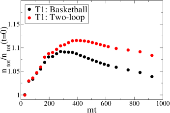
Surprisingly, the process of equilibration in the two-loop approximation seems to occur almost as fast as in the Basketball case. The same holds for the chemical equilibration that takes place at later stages of the evolution, as one can see in Fig. 6. As in the symmetric case, chemical equilibration is very slow, which impedes the approach to complete equilibrium.

Fig. 6.: Evolution of total particle number density $n_{\mbox{\tiny tot}}$ for the two-loop and Basketball approximations.

5 Conclusions

In this work several truncations of the 2PI effective action have been used to study equilibration in $\varphi^{4}$ theory in 3+1 dimensions. Early in the evolution, the distribution function and dispersion relation stabilize and take equilibrium-like forms due to a relatively fast kinetic equilibration (see also [14]). This occurs for both the two-loop and Basketball approximations, which take scattering into account. Surprisingly, equilibration is equally rapid in both approximations. An analysis of damping rates of distrubances close to equilibrium leads to a similar conclusion [10].

The pre-equilibrated state has not completely lost the memory of the initial state. In particular, initial conditions with different total particle number pre-equilibrate to different states. The later approach to complete equilibrium is very slow and mainly determined by the time scales associated with chemical equilibration.

References

• [1] U. W. Heinz and P. F. Kolb, Nucl. Phys. A 702 (2002) 269
• [2] D. Molnar and M. Gyulassy, Nucl. Phys. A 697 (2002) 495
• [3] G. Baym, Phys. Rev.  127 (1962) 1391.
• [4] J. Berges and J. Cox, Phys. Lett. B 517 (2001) 369
• [5] G. Aarts, D. Ahrensmeier, R. Baier, J. Berges and J. Serreau, Phys. Rev. D 66 (2002) 045008
• [6] F. Cooper, J. F. Dawson and B. Mihaila, Phys. Rev. D 67 (2003) 056003
• [7] S. Juchem, W. Cassing and C. Greiner, Phys. Rev. D 69 (2004) 025006
• [8] J. Berges, S. Borsanyi and J. Serreau, Nucl. Phys. B 660 (2003) 51
• [9] A. Arrizabalaga and J. Smit, Phys. Rev. D 66 (2002) 065014
• [10] A. Arrizabalaga, J. Smit and A. Tranberg, Phys. Rev. D 72 (2005) 025014
• [11] J. M. Cornwall, R. Jackiw and E. Tomboulis, Phys. Rev. D 10 (1974) 2428.
• [12] N. P. Landsman and C. G. van Weert, Phys. Rept.  145, 141 (1987).
• [13] J. Berges, S. Borsanyi, U. Reinosa and J. Serreau, arXiv:hep-ph/0503240.
• [14] J. Berges, S. Borsanyi and C. Wetterich, Phys. Rev. Lett.  93 (2004) 142002